Quadratic Programming Vision-Based Control of a Scale-Model Autonomous Vehicle Navigating in Intersections

Abstract

This paper presents an optimal control for autonomous vehicles navigating in intersection scenarios. The proposed controller is based on solving a Quadratic Programming optimization technique to provide a feasible control signal respecting actuator constraints. The proposed controller was implemented in a scale-sized vehicle and is executed using only on-board perception and computing systems to retrieve the state dynamics, i.e., an inertial measurement unit and a monocular camera, to compute the estimated states through intelligent computer vision algorithms. The stability of the error signals of the closed-loop system was proved both mathematically and experimentally, using standard performance indices for ten trials. The proposed technique was compared against LQR and MPC strategies, showing 67% greater accuracy than the LQR approach and 53.9% greater accuracy than the MPC technique, while turning during the intersection. Moreover, the proposed QP controller showed significantly greater efficiency by reducing the control effort by 63.3% compared to the LQR, and by a substantial 78.4% compared to the MPC. These successful results proved that the proposed controller is an effective alternative for autonomously navigating within intersection scenarios.

1. Introduction

Over the past decade, autonomous driving systems have attracted increasing interest from both industry and research communities. These systems are a cornerstone for reducing traffic accidents, improving traffic efficiency, and enabling new forms of mobility. A key factor in the development of autonomous driving systems is the design of controllers capable of safely and accurately following desired trajectories, especially in complex urban environments [1].

Most of the advances in the development of self-driving vehicles have started as research projects using scale-sized prototypes, as is the case of the project reported in this work, which was developed in academic laboratory conditions using a scale-sized car, where the road surface is flat and there are no adverse atmospheric conditions; this work is focused in the problem of controlling this car to manage the navigation in standard urban intersections.

Intersections are particularly critical points in traffic networks, often leading to delays and accidents. For this reason, Autonomous Intersection Management (AIM) is an active area of research, where path planning is performed for each vehicle in cruising scenarios, and vehicle movements are executed through automation [2,3].

Considering the literature reported so far, the research gaps found are the following: (1) Control systems for navigating in intersections require oversimplified models and complex sensing and communication schemes. (2) Several strategies neglect the lower-level vehicle controller implementation details and integration. (3) There is a substantial predominance on simulation-based validation. (4) The use of off-board computing and sensing reduces the reliability on real-world scenarios. (5) The prevalently employed controllers are not capable to handle real-world constraints, such as actuator limits.

Aiming to fill out the aforementioned research gaps, this work presents an autonomous control architecture that enables lane following and intersection navigation using only an inertial measurement unit (IMU), a monocular camera, and computer vision algorithms. The system integrates visual processing for lane and intersection detection, vehicle state estimation, and a Quadratic Programming (QP)-based controller that determines the vehicle’s actions in real time, which in contrast to standard optimal controllers such as the linear quadratic regulator (LQR) or predictive algorithms, allows the handling of inequality constraints with less computational burden, directly computing the control input without a prediction horizon, as is presented in [4]. The proposed architecture consists of several modules: a visual perception module that processes images captured by a forward-facing camera to identify lane markings; a Convolutional Neural Network (CNN) to detect cruising scenarios; a state estimation module that interprets visual and inertial data to define the vehicle’s current and desired states; and a switching controller module that implements an optimal control scheme based on QP to compute steering and velocity commands, enabling the vehicle to achieve navigation objectives while satisfying the imposed actuator constraints.

This paper is organized as follows. Section 2 presents the related work, while Section 3 presents dynamic model of the vehicle and the hardware/software architecture employed. Section 4 details the visual feedback pipeline, covering road perspective correction, state estimation, and CNN-based scene classification. Section 5 describes the proposed QP controller and its stability. Section 6 reports the experimental results obtained in real-world navigation scenarios, comparing the proposed QP controller against LQR and Model-Predictive Control (MPC) baselines. Finally, Section 7 summarizes the main conclusions and outlines future research directions.

2. Related Work

The navigation control of autonomous vehicles is taken for granted in navigation scenarios, so most research is instead dedicated to traffic monitoring and control, thereby leaving aside the potential implications of the lower-level controller implementation. Nonetheless, some authors have attempted to solve the navigation in intersections control problem, so diverse schemes have been reported in the literature so far, such as PID, Optimal Control, and MPC. However, most studies in the literature develop control laws based on overly simplified models, requiring a constant communication between vehicles and others agents, also assuming that many vehicle states are measured. In addition, a substantial majority of these results are obtained solely through numerical simulations, leaving aside the feedback state measurement or estimation algorithms [1,3,5,6,7,8,9].

For example, Vitale et al. [9], propose a centralized control method to manage traffic at road intersections. Their scheme solves an optimization problem where the states include the position and velocity of the vehicles, and the output is an acceleration profile for each vehicle within the intersection. They present simulation results showing that vehicles can cross safely without collisions, maintaining a safety distance of six meters. However, their system requires constant and perfect communication between vehicles, and the model assumes that vehicles cannot make turns. These limitations hinder its applicability in real-world environments.

Another strategy is presented by Ding et al. [8], where a control system for autonomous vehicles is used to perform turning maneuvers at intersections. In their work, vehicles communicate with Road Side Units and with each other to obtain the position and velocity of nearby vehicles. Using a Model-Predictive Control (MPC) scheme, each vehicle calculates its acceleration and steering angle to execute left turns, right turns, or U-turns while cruising—adjusting its speed accordingly and maintaining a safe distance. Nevertheless, this system relies on a communication infrastructure that is subject to latency, data loss, and limited coverage. Additionally, high precision in vehicle positioning is required.

Similarly, Meng and Cassandras [7] propose a real-time optimal control method for autonomous vehicles approaching signalized intersections under free-flow conditions. The goal is to minimize both energy consumption and travel time while avoiding idle stops. By leveraging vehicle-to-infrastructure (V2I) communication, their algorithm dynamically adjusts vehicle speed profiles to enable non-stop intersection crossings. The control formulation assumes a single autonomous vehicle operating in free-flow mode, excluding interaction effects, lateral maneuvers, and lane constraints. The framework also depends on precise V2I signal timing, and potential discomfort caused by acceleration spikes near the onset of green lights may require additional buffering strategies. Furthermore, the method assumes straight-line motion without turns, and does not address the feasibility of lane changes.

In contrast, the navigation of autonomous vehicles in cruising scenarios without external communication systems has been less explored in the literature [10,11,12,13]. For example, Pourjafari et al. [13] propose a predictive scheme for navigating unsignalized road intersections. Their objective is to predict the behavior of other vehicles, determine the order of passage at collision points, and compute an acceleration profile for the ego vehicle. The proposed control method considers multiple constraints, while the states of other vehicles are estimated using Long Short-Term Memory (LSTM) and Graph Neural Networks. Ultimately, they present simulation results based on 250 real-world scenarios, demonstrating that the vehicle can navigate safely and, in some cases, outperform human drivers. However, the method relies heavily on the precision of neural network data and has not been experimentally validated.

On the other hand, Zannatha et al. [12,14] have presented a modular navigation system for scaled autonomous vehicles operating in urban environments. Their approach integrates route planning using Dijkstra’s algorithm, geometric trajectory generation adapted to intersection geometry, and a hybrid navigation controller that combines odometry-based Stanley steering with trapezoidal velocity profiling. All modules were validated in a ROS–Gazebo simulator within a 2D urban environment featuring 90° intersections and a uniform road layout. However, the method assumes idealized urban geometry—excluding roundabouts, diagonal roads, or variable curvatures. Only a single vehicle is considered, with no dynamic agents or multi-agent coordination. Their controller relies heavily on odometry, and lane perception is limited to geometric assumptions.

Sezer et al. [11] present a decision-making system for autonomous vehicles that infers the intentions of other drivers and makes safe and efficient decisions to cross or merge at unsignalized T-intersections. To achieve this, they use a probabilistic model known as a Mixed Observability Markov Decision Process (MOMDP). The system was implemented on an autonomous vehicle (a modified golf cart) and tested at a real intersection on the campus of the National University of Singapore. In their experiments, the system successfully detected changes in the intentions of aggressive drivers, avoided collisions, and chose safe actions. However, the model assumes that the positions of both the autonomous and human-driven vehicles are perfectly observable, which may not hold in practice due to sensor errors, occlusions, or adverse conditions. Additionally, the approach is computationally expensive.

Additionally, control strategies based on Quadratic Programming are attractive because they yield optimal solutions while simultaneously accounting for state and control input constraints. However, this approach has been primarily used for trajectory tracking [15,16,17,18,19], and mostly present only simulation results. In Lee [19], a soft-constrained variant of the constrained iterative Linear Quadratic Regulator (CILQR) algorithm is proposed for lane-keeping control in autonomous vehicles. The controller introduces slack variables to relax state and input constraints within a barrier-function-based optimization framework, aiming to suppress steering jitter without relying on external filters. Performance is validated through numerical simulations and vision-based experiments in perturbed environments.

Similarly, Yuan and Zhao [17] present a hierarchical trajectory-tracking controller for autonomous vehicles that couples lateral and longitudinal dynamics using a hybrid Linear LQR and MPC framework. The architecture integrates an Extended Kalman Filter (EKF) observer to estimate driving states (e.g., velocity and yaw rate), aiming to improve accuracy under state uncertainty. The framework is validated using CarSim–Simulink co-simulation across various speed scenarios and benchmarked against a classical MPC-only control scheme. However, the EKF’s accuracy depends on well-tuned noise parameters, which may vary across scenarios.

Considering the published results regarding autonomous vehicles control in intersections so far, this paper presents a low-level control system that only uses on-board sensors and computers to accurately navigate in intersections, avoiding communication between agents and external sensing in contrast to the works found in the literature. Moreover, the proposed control scheme takes into account actuator constraints and it is implemented on a real scale-model vehicle, which are clear advantages over the state of the art.

3. Autonomous Vehicle Description

3.1. Vehicle Dynamics

The motion of autonomous vehicles is typically modeled using dynamic equations that capture the behavior of the car’s body and its interaction with the environment. A widely adopted approach is the so-called bicycle model, which simplifies the car dynamics while preserving key characteristics such as turning radius, slip angle, etc. [20]. This model is crucial for designing and implementing predictive control algorithms. Consider Figure 1, where both the longitudinal and lateral velocities, $V_x$ and $V_y$, are shown, as well as the geometric parameters of the vehicle detailed in

Table 1. Parameter description.

Symbol	Description
$C_{cf},C_{cr}$	Cornering stiffness of front and rear tires
${\ell }_f,{\ell }_r$	Distance from Center of Mass to front and rear axles
m	Mass of the vehicle
$I_z$	Yaw moment of inertia
$V_x$	Longitudinal velocity

. The lateral dynamics of the vehicle are governed by the following force and moment equations,

$$\begin{array}{cc}\hfill m{\dot{V}}_y\left(t\right)& =F_{yf}+F_{yr} ,\hfill \\ \hfill I_z\ddot{\psi }\left(t\right)& =l_f{F}_{yf}-l_r{F}_{yr} ,\hfill \end{array}$$

(1)

where $F_{yf}$ and $F_{yr}$ are the lateral tire forces at the front and rear wheels, respectively, which in turn are given by

$$\begin{array}{cc}\hfill F_{yf}& =2C_{cf}(\delta -{\theta }_f) ,\hfill \\ \hfill F_{yr}& =2C_{cr}(-{\theta }_r) .\hfill \end{array}$$

(2)

The angles ${\theta }_f$ and ${\theta }_r$, known as the tire slip angles. After some algebra and identities it follows that

$$\begin{array}{cc}\hfill tan\left({\theta }_f\right)& ={\displaystyle \frac{V_y+l_f\dot{\psi }}{V_x}} ,\hfill \\ \hfill tan\left({\theta }_r\right)& ={\displaystyle \frac{V_y-l_r\dot{\psi }}{V_x}} ,\hfill \end{array}$$

(3)

so the lateral dynamics can be linearized as follows about small values of ${\theta }_f$ and ${\theta }_r$

$$\begin{array}{cc}\hfill {\dot{V}}_y\left(t\right)& =-\left({\displaystyle \frac{2C_{cf}+2C_{cr}}{m{V}_x}}\right)V_y-\left(V_x+{\displaystyle \frac{2C_{cf}{l}_f+2C_{cr}{l}_r}{m{V}_x}}\right)\dot{\psi }+\left({\displaystyle \frac{2C_{cf}}{m}}\right)\delta ,\hfill \\ \hfill \ddot{\psi }\left(t\right)& =-\left({\displaystyle \frac{2C_{cf}{l}_f-2C_{cr}{l}_r}{I_z{V}_x}}\right)V_y-\left({\displaystyle \frac{2C_{cf}{l}_f^2+2C_{cr}{l}_r^2}{I_z{V}_x}}\right)\dot{\psi }+\left({\displaystyle \frac{2C_{cf}{l}_f}{I_z}}\right)\delta .\hfill \end{array}$$

(4)

Afterwards, defining the tracking errors

$$\begin{array}{cc}\hfill e_y& =y-y_{ref} ,\hfill \\ \hfill e_{\psi }& =\psi -{\psi }_{ref} ,\hfill \\ \hfill \Rightarrow {\dot{e}}_y& =V_y+V_x{e}_{\psi }\mathrm{with}: {\dot{y}}_{ref}=-V_x{e}_{\psi } ,\hfill \\ \hfill {\dot{e}}_{\psi }& =\dot{\psi }-{\dot{\psi }}_{ref} ,\hfill \end{array}$$

and folding the dynamic equations into them it yields

$$\begin{array}{cc}\hfill {\ddot{e}}_y=& -\left({\displaystyle \frac{2C_{cf}+2C_{cr}}{m{V}_x}}\right)V_y-\left(V_x+{\displaystyle \frac{2C_{cf}{l}_f+2C_{cr}{l}_r}{m{V}_x}}\right)\dot{\psi }+\left({\displaystyle \frac{2C_{cf}}{m}}\right)\delta +V_x{\dot{e}}_{\psi }\hfill \\ \hfill =& -\left({\displaystyle \frac{2C_{cf}+2C_{cr}}{m{V}_x}}\right)({\dot{e}}_y-V_x{e}_{\psi })-\left(V_x+{\displaystyle \frac{2C_{cf}{l}_f+2C_{cr}{l}_r}{m{V}_x}}\right)({\dot{e}}_{\psi }+{\dot{\psi }}_{ref})\hfill \\ & +\left({\displaystyle \frac{2C_{cf}}{m}}\right)\delta +V_x{\dot{e}}_{\psi } ,\hfill \end{array}$$

$$\begin{array}{cc}\hfill {\ddot{e}}_{\psi }=& -\left({\displaystyle \frac{2C_{cf}{l}_f-2C_{cr}{l}_r}{I_z{V}_x}}\right)V_y-\left({\displaystyle \frac{2C_{cf}{l}_f^2+2C_{cr}{l}_r^2}{I_z{V}_x}}\right)\dot{\psi }+\left({\displaystyle \frac{2C_{cf}{l}_f}{I_z}}\right)\delta -{\ddot{\psi }}_{ref}\hfill \\ \hfill =& -\left({\displaystyle \frac{2C_{cf}{l}_f-2C_{cr}{l}_r}{I_z{V}_x}}\right)({\dot{e}}_y-V_x{e}_{\psi })-\left({\displaystyle \frac{2C_{cf}{l}_f^2+2C_{cr}{l}_r^2}{I_z{V}_x}}\right)({\dot{e}}_{\psi }+{\dot{\psi }}_{ref})\hfill \\ & +\left({\displaystyle \frac{2C_{cf}{l}_f}{I_z}}\right)\delta -{\ddot{\psi }}_{ref} .\hfill \end{array}$$

Finally, considering $V_x$ constant, the derivatives of the reference signals are set to zero (position regulation), and after rearranging terms, the state-space representation of the vehicle model becomes

$$\left(\begin{array}{c}{\dot{e}}_y\\ {\ddot{e}}_y\\ {\dot{e}}_{\psi }\\ {\ddot{e}}_{\psi }\end{array}\right)=\underset{A}{\underbrace{\left(\begin{array}{cccc}0& 1& 0& 0\\ a_{21}& 0& a_{23}& a_{24}\\ 0& 0& 0& 1\\ a_{41}& 0& a_{43}& a_{44}\end{array}\right)}}\underset{x}{\underbrace{\left(\begin{array}{c}{e}_y\\ {\dot{e}}_y\\ e_{\psi }\\ {\dot{e}}_{\psi }\end{array}\right)}}+\underset{B}{\underbrace{\left(\begin{array}{c}0\\ b_2\\ 0\\ b_4\end{array}\right)}}\delta .$$

(5)

The expressions of matrices A and B elements are listed in

Table 2. Elements of matrices A and B.

Element	Value	Element	Value
$a_{21}$	${\displaystyle \frac{2C_{cf}+2C_{cr}}{m{V}_x}}$	$a_{43}$	${\displaystyle \frac{2C_{cf}{\ell }_f-2C_{cr}{\ell }_r}{I_z}}$
$a_{23}$	${\displaystyle \frac{2C_{cf}+2C_{cr}}{m}}$	$a_{44}$	${\displaystyle \frac{-2C_{cf}{\ell }_f^2+2C_{cr}{\ell }_r^2}{I_z{V}_x}}$
$a_{24}$	${\displaystyle \frac{-2C_{cf}{\ell }_f+2C_{cr}{\ell }_r}{m{V}_x}}$	$b_2$	${\displaystyle \frac{2C_{cf}}{m}}$
$a_{41}$	${\displaystyle \frac{-2C_{cf}{\ell }_f+2C_{cr}{\ell }_r}{I_z{V}_x}}$	$b_4$	${\displaystyle \frac{2C_{cf}{\ell }_f}{I_z}}$

.

Then, the discrete-time version of (5) is given by

$$x_{k+1}=A_d{x}_k+B_d{\delta }_k ,$$

(6)

where $A_d=e^{hA}$ and $B_d={\int }_0^h{e}^{sA}B ds$ for a given sampling period h, with $x_0$ denoting the initial measured errors vector within the range $-7.2$ cm $\le e_{y_0}\le 15.1$ cm and $-0.37$ rad $\le e_{{\psi }_0}\le 0.25$ rad. Such a model is useful to design the control system in discrete time, which in turn will be executed as a program within an embedded computer.

3.2. The AutoMiny 4.0

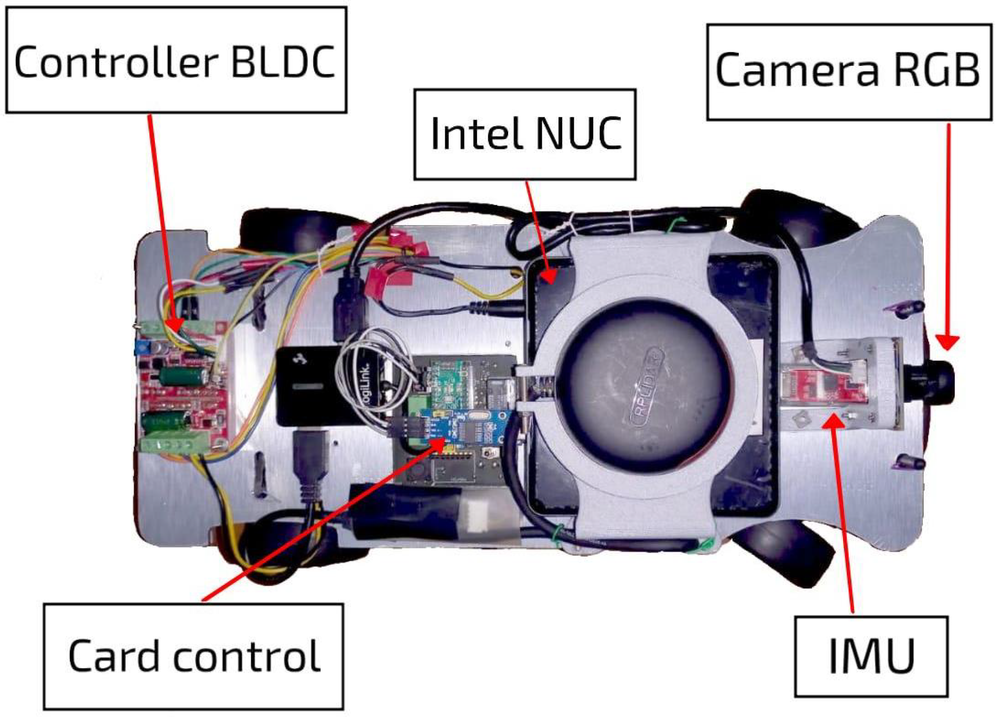
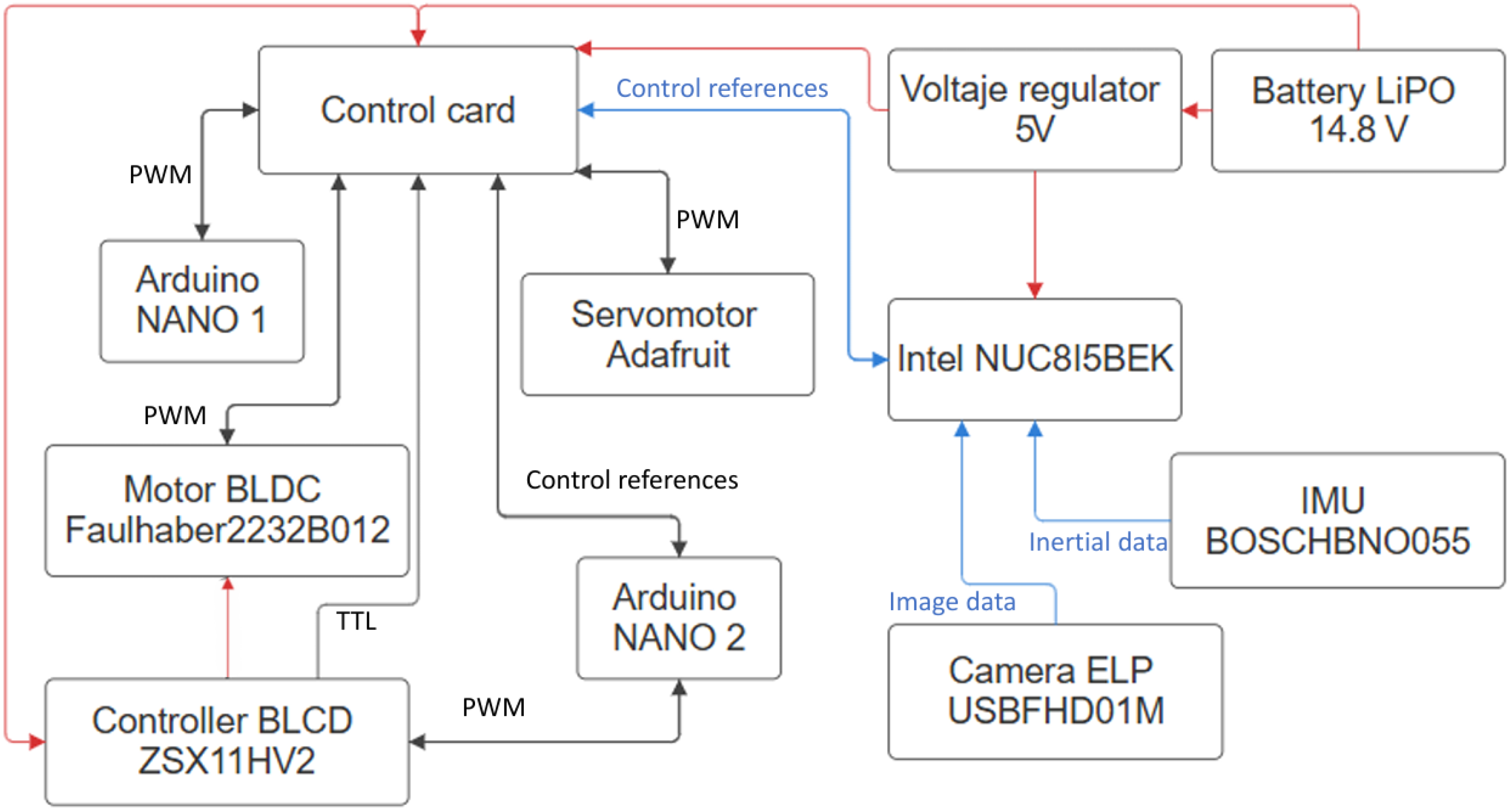
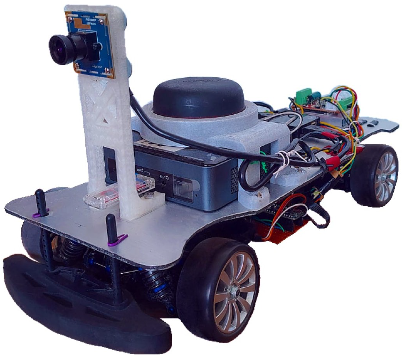
The experimental platform in study is the AutoMiny 4.0, which is a miniature autonomous vehicle designed for research and educational purposes. It integrates multiple sensors and actuators that are necessary for autonomous navigation (https://autominy.github.io/AutoMiny/, accessed on 30 July 2025) [14]. The AutoMiny vehicle is illustrated in Figure 2. It is equipped with an ELP USBFHD01M fisheye camera (Ailipu Technology Inc., Shenzhen, China) to provide a wide field of view, a ${360}^{\circ }$ A2M8 LiDAR (SLAMTEC, Shanghai, China) for obstacle detection, and a BNO055 IMU (Bosch Sensortec, Reutlingen, Germany) for orientation and motion sensing. For actuation, it uses a TowerPro SG-5010 servomotor (Tower Pro, Kowloon, Hong Kong) for steering and a 2232B 012 BX4 SC (Faulhaber, Schönaich, Germany) brushless DC motor for traction. Moreover, an Arduino Nano manages the low-level motor control. Additionally, the perception, control, and navigation algorithms are executed by an Intel NUC8i5BEK mini-PC (Intel, Santa Clara, CA, USA), running Ubuntu 18.04 with the Robot Operating System (ROS). All components are mounted on a rigid Alucobond chassis. Such components are shown in Figure 3, whereas Figure 4 illustrates the system block diagram representing the signal interchange between on-board electronic devices.

3.3. ROS Software Configuration

The ROS Melodic framework provides a robust infrastructure for distributed integration and communication among sensors, actuators, and control algorithms. Furthermore, it leverages a publisher-subscriber communication model, enabling data exchange between nodes through topics, allowing both temporal and spatial decoupling between components. The nodes implemented to execute the control of the AutoMiny are as follows:

• camera_ELP: Captures images from the front-facing fisheye lens camera at a frequency of 30 Hz and publishes them on the topic Image_Raw.
• bno_055: Collects inertial data from the BNO055 IMU sensor, including acceleration, angular velocity, and orientation (quaternion or Euler angles). The processed data is published on the topic bno_055/output.
• QP_control: Receives camera and IMU data from Image_Raw and bno_055/output, respectively. It implements a convolutional neural network (CNN) to classify the scene as either “in intersection” or “out of intersection”. Based on this classification, it switches between two QP-based controllers, each tailored to one of the cases. At the end, it publishes the steering angle $\delta$ on steering, and the desired longitudinal speed $V_x$ on speed.
• gps_pose: Receives ground-truth camera images and performs visual processing, including color segmentation, homography transformation, and geometric feature extraction. It then provides absolute position and orientation data for experimental validation. The 2D pose is published on the topic pose_car, and the error states $e_y$ and $e_{\psi }$ are published on error_car.
• LQR_control and MPC_control: These nodes implement alternative control strategies for trajectory tracking using LQR and MPC, respectively. Both nodes receive reference trajectories and vehicle state information, and output control commands. The steering angle $\delta$ and desired speed $V_x$ are published on the topics steering and speed, respectively.

The interaction between the aforesaid ROS nodes is presented in Figure 5 for the LQR and MPC approaches, and in Figure 6 for the QP controller, where it can be clearly shown that the proposed QP does not depend on a ground-truth external measurement (gps_pose), but only gets feedback from the on-board sensors.

4. Visual Feedback

4.1. Road Perspective Correction

Consider the 2D plane captured by the on-board camera, also known as the image space, denoted by

$$I_{sp}\triangleq \left\{(u,v)\in {\mathbb{Z}}_{+}^2|u\in [1,p],v\in [1,q]\right\}$$

(7)

where u and v denote the horizontal and vertical pixel coordinates, and $p\times q$ is the image resolution. Also consider the coordinate frame associated with the road, denoted by $\left\{W\right\}$. The trajectory coordinates of the self-driving car are defined in the road frame $\left\{W\right\}$ and expressed in meters. However, in the corresponding image, this trajectory appears distorted due to the projection model of the camera and is expressed in pixels. Since the vehicle control is computed in the image space, it is necessary to establish a model that relates the coordinates in the road frame $\left\{W\right\}$ to those in the image space $I_{sp}$ (in pixels).

Such a model corresponds to the camera projection applied to a 2D plane (the road surface), rather than the general 3D workspace model. This reduced model is known as a homography, and it is obtained by projecting planar world points into the image using the camera model, which is defined by three matrices: the intrinsic calibration matrix, the perspective projection, and the homogeneous transformation representing the pose of the camera with respect to the world frame. The full projection model is given by

$$\left[\begin{array}{c}u\\ v\\ 1\end{array}\right]=\underset{K}{\underbrace{\left[\begin{array}{ccc}{k}_x& 0& c_x\\ 0& k_y& c_y\\ 0& 0& 1\end{array}\right]}}\left[\begin{array}{cccc}1& 0& 0& 0\\ 0& 1& 0& 0\\ 0& 0& 1& 0\end{array}\right]\left[\begin{array}{cc}{R}_{3\times 3}& t_{3\times 1}\\ 0_{1\times 3}& 1\end{array}\right]\left[\begin{array}{c}{X}^{\prime }\\ Y^{\prime }\\ Z^{\prime }\\ 1\end{array}\right] ,$$

(8)

where $k_x$, $k_y$, $c_x$, and $c_y$ are real scalars representing the intrinsic camera parameters, $R\in \mathcal{SO}\left(3\right)$ is the rotation matrix, and $t\in {\mathbb{R}}^3$ is the translation vector, both defining the pose of the camera with respect to the world frame. It is important to note that the world frame axes are selected so that axis z is pointed down to make the correspondence between the coordinates in the world and image frames easier. Now, if the points of interest lie on the plane defined by ${(X^{\prime },Y^{\prime },0,1)}^T$, the (8) projection model is reduced to an homography as  

$$\begin{array}{ccc}\hfill \left[\begin{array}{c}u\\ v\\ 1\end{array}\right]& =& \left[\begin{array}{ccc}{k}_x& 0& c_x\\ 0& k_y& c_y\\ 0& 0& 1\end{array}\right]\left[\begin{array}{cc}{R}_{2\times 2}& t_{2\times 1}\\ 0_{1\times 2}& 1\end{array}\right]\left[\begin{array}{c}{X}^{\prime }\\ Y^{\prime }\\ 1\end{array}\right] ,\hfill \\ \hfill & =& \left[\begin{array}{ccc}{k}_x& 0& c_x\\ 0& k_y& c_y\\ 0& 0& 1\end{array}\right]\left[\begin{array}{ccc}cos\left(\theta \right)& sin\left(\theta \right)& t_x\\ cos\left(\theta \right)& -sin\left(\theta \right)& t_y\\ 0& 0& 1\end{array}\right]\left[\begin{array}{c}{X}^{\prime }\\ Y^{\prime }\\ 1\end{array}\right]=H\left[\begin{array}{c}{X}^{\prime }\\ Y^{\prime }\\ 1\end{array}\right] ,\hfill \end{array}$$

(9)

where $(t_x,t_y,\theta )$ is the vehicle pose and H is the homography matrix. Given a set of points on the road surface with known world coordinates (in meters) and their corresponding image coordinates (in pixels), obtained from a known pose (used to initialize the car odometry), it is possible to estimate the inverse homography matrix used to reconstruct the workspace corresponding only to the road surface

$$\left[\begin{array}{c}{X}^{\prime }\\ Y^{\prime }\\ 1\end{array}\right]=H^{-1}\left[\begin{array}{c}u\\ v\\ 1\end{array}\right] .$$

(10)

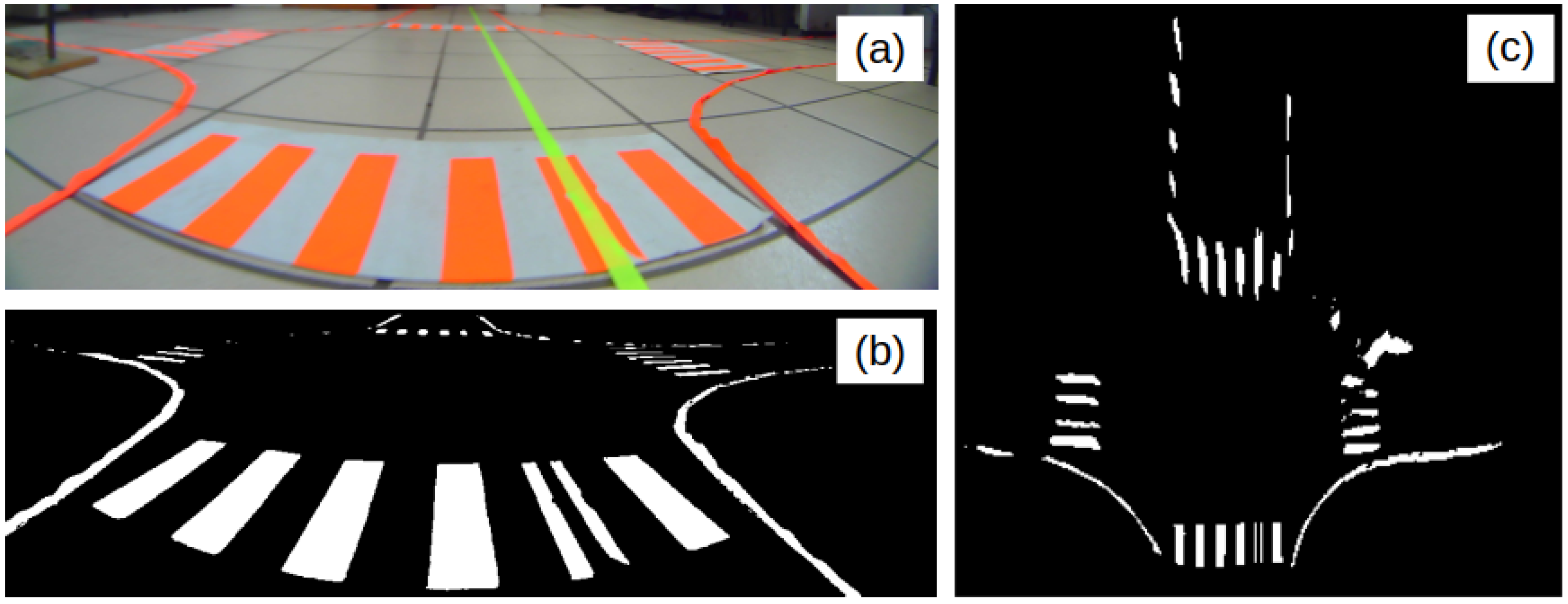
Homography matrix and its inverse are functions of the actual vehicle pose $(t_x,t_y,\theta )$. Even if these matrices are identified in a specific part of the workspace, i.e., for a specific pose $(R_{2\times 2},t_{2\times 1})$, it can be used all over the road surface because the absolute coordinates of the features on the road surface are not needed and only their relative position respect to the car is. In addition, the image analysis to find features in the workspace (e.g., lane markings, intersection, horizontal signage, etc.) is applied only in a relevant area of the reconstructed space in front of the car, so only a rectangle of 3.5 m × 2.1 m in front of the vehicle is used. Thus, features in the workspace (e.g., lane markings, intersection, horizontal signage) can be localized and measured and lateral errors can be evaluated through some image processing and analysis algorithms, as described in the following sections. In Figure 7, the steps to obtain the homography transformation of the road are shown.

4.2. Ground-Truth System

Ground truth refers to accurate and verified information used as a reference to evaluate the performance of computer vision models. It plays a critical role in a model’s ability to generalize and make correct decisions in real-world scenarios by reducing errors and biases, leading to a balanced decision-making and improving prediction accuracy.

Figure 8 illustrates the system’s processing pipeline, which begins with image acquisition using a fisheye camera mounted on the ceiling. The captured images are corrected to eliminate tangential lens distortion and subsequently transformed into a top-down (bird’s-eye) view using the homography transformation (10). Afterwards, a color-based segmentation is applied to identify markers placed on the vehicle, and finally, image moments are computed from these segmented regions to determine the vehicle’s position and orientation within the environment by locating the centroids of each marker color.

Figure 9 shows the colored markers placed on the top of the vehicle (e.g., green and blue patches) to facilitate visual localization via segmentation. The left image shows the vehicle in the physical environment, while the right image displays the homography-transformed top-down view, where the vehicle’s position and orientation can be clearly observed. This system is essential for quantifying tracking errors and validating the performance of the implemented controllers.

4.3. Convolutional Neural Network

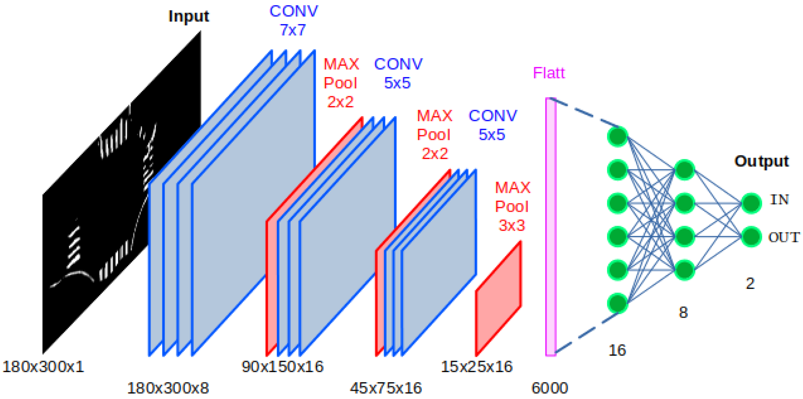
In order to select the type of controller that the AutoMiny must follow, a Convolutional Neural Network (CNN) was trained to detect whether the car is inside or outside the intersection. The input to the CNN is an homography-cropped image of size $180\times 300\times 1$, which is classified into one of two categories: $\mathbf{In}$ or $\mathbf{Out}$. The architecture of the network is shown in Figure 10, where it can be appreciated that the input image is the segmented homography. Moreover, the training dataset was built by recording road images while the car navigated through the intersection. In each image, the lane markings were segmented, and an homography transformation was applied. A total of 5636 images were used for training, and 628 were used for validation. Figure 11 shows three examples of each class. After training, the network achieved an accuracy of $\mathrm{97.9\%}$. The confusion matrix for the validation set is shown in Figure 12.

4.4. States Computation Through Visual Feedback

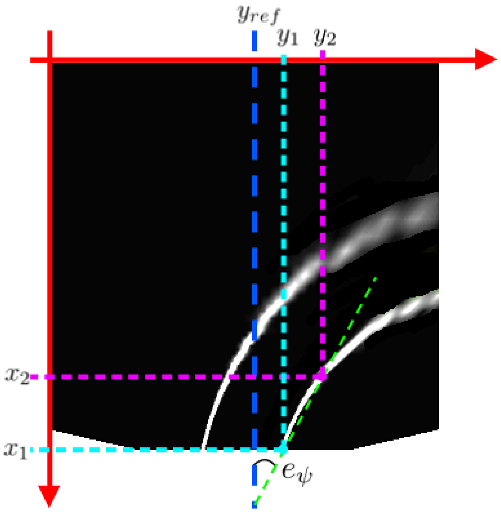
Recalling the error dynamics (6), the lateral error $e_y$ and heading error $e_{\psi }$ are measured using the homography of the road. Specifically, each image captured by the on-board camera undergoes an homography transformation, followed by a color segmentation step to extract the lane markings. Then, two points on the right lane line are identified using a line detector. These points, denoted as $(x_1,y_1)$ and $(x_2,y_2)$, are used to compute the slope m of a secant line. The lateral and heading errors are then calculated as $e_y=y_1-y_{ref}$ and $e_{\psi }=-arctan\left(m\right)$, respectively. These variables are illustrated in Figure 13, where its relation with the visual information can be appreciated. Notice that the states $e_y$ and $e_{\psi }$ are according to the image frame as is explained in Section 4.

5. Quadratic-Programming Control

Quadratic Programming (QP) is a type of mathematical optimization problem in which the objective function is quadratic and the constraints are linear. It is a widely used control strategy because it allows for the explicit handling of constraints on system dynamics, states, and actuator limits, which cannot be directly handled by traditional optimal control approaches like the Linear Quadratic Regulator (LQR). The objective function typically reflects goals such as minimizing control effort or tracking error, while the constraints can include the system dynamics, actuator saturation, state bounds, and safety requirements.

Considering the error dynamics (6), and the control problem of leading to zero the states, a cost objective function can be defined as

$$\left\{\begin{array}{cc}\hfill J\left({\delta }_k\right)& =\sum _{k=0}^{\infty }{x}_k^{T}Q{x}_k+R{\delta }_k^2+g\left({\delta }_k\right) ,\hfill \\ \hfill g\left({\delta }_k\right)& =\rho ·max(0,|{\delta }_k{|-1)}^2 ,\hfill \end{array}\right.$$

(11)

where $Q\in {\mathbb{R}}^{4\times 4}$ is a positive definite diagonal matrix and $R,\rho \in \mathbb{R}$ are positive scalars. The penalty constant $\rho$ is obtained by varying its value while solving the optimization problem in simulation, it can be later implemented in the real vehicle. Moreover, $g\left({\delta }_k\right)$ is a differentiable quadratic function that penalizes violations of the actuator constraints. This approach is referred to as a soft constraint [21,22], which introduces a weighted penalty whenever the control input ${\delta }_k$ exceeds the admissible range, which in this case is ${\delta }_k\in [-1.5,1.5]$, resulting from the admissible values of the ROS topic steering, which in turn maps the corresponding PWM value to move the servomotor within a $-0.4$ to $0.4$ radians or $67.8$ to $112.2$ deg (0 deg steering corresponds to 90 deg servomotor shaft).

Given a control horizon $N_h$, at iteration k, it is possible to estimate future states $x_{k+1}, x_{k+2},\dots ,x_{k+N_h}$ by applying (6) iteratively. Then, the estimated immediate cost from time step k is

$$J_k=\sum _{j=1}^{N_h}{x}_{k+j}^{T}Q{x}_{k+j}+R{\delta }_{k+j}^2+g\left({\delta }_{k+j}\right) .$$

(12)

Assuming that this has the form ${\delta }_{k+j}=-K_{k+j}{x}_{k+j}$, it is possible to find a set of optimal gains $K_{k+j}$ that minimize (12) using a numerical solver, such as the Broyden–Fletcher–Goldfarb–Shanno (BFGS) (https://docs.scipy.org/doc/scipy/reference/optimize.minimize-bfgs.html, accessed on 2 October 2025) [23]. Then, the control problem formulated as a QP is

$$\begin{array}{cc}\underset{x}{\min }& \sum _{j=1}^{N_h}{x}_{k+j}^{T}Q{x}_{k+j}+R{\delta }_{k+j}^2+g\left({\delta }_{k+j}\right) \hfill \\ s.t.& -1.5\le \delta (k+j)\le 1.5 .\hfill \end{array}$$

(13)

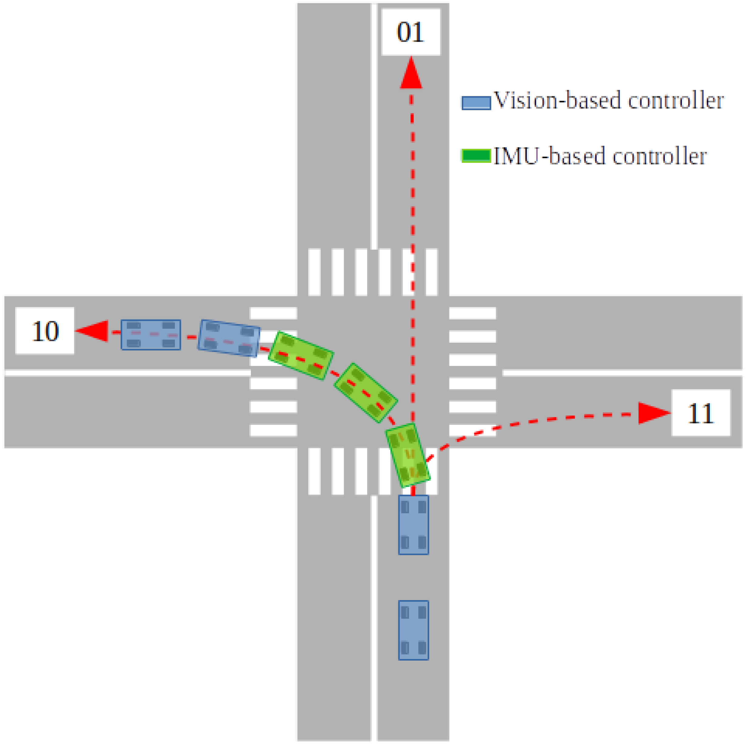
In practice, two types of controllers are used for navigation. The first is a vision-based controller for lane keeping, using the lane markings as reference. From the images captured by the on-board camera, it is possible to measure the states $e_y$ and $e_{\psi }$ (as detailed in Section 4.4). In general, this is sufficient to follow the road. However, at an intersection, there are three possible paths and insufficient floor markings to reliably estimate the vehicle’s position and orientation. For this reason, a second controller with IMU-based feedback was designed. This controller records the vehicle’s yaw angle ${\psi }_0$ just before entering the cruise and computes the orientation error $e_{\psi }$ as follows:

$$e_{\psi }=\psi -{\psi }_{ref},\mathrm{where}{\psi }_{ref}=\left\{\begin{array}{cc}{\psi }_0\hfill & \mathrm{if}\mathrm{going}\mathrm{straight}(\mathrm{case}01)\hfill \\ {\psi }_0+{\displaystyle \frac{\pi }{2}}\hfill & \mathrm{if}\mathrm{turning}\mathrm{left}(\mathrm{case}10)\hfill \\ {\psi }_0-{\displaystyle \frac{\pi }{2}}\hfill & \mathrm{if}\mathrm{turning}\mathrm{right}(\mathrm{case}11)\hfill \end{array}\right.$$

(14)

After computing $K_{\mathrm{imu}}$ and $K_{\mathrm{vis}}$ by minimizing the immediate cost in (12), a controller switching strategy was implemented as follows:

$$\begin{array}{cc}\hfill {\delta }_k& =\underset{K_k}{\underbrace{\left(-{\zeta }_k{K}_{\mathrm{imu}}+(1-{\zeta }_k)K_{\mathrm{vis}}\right)}}{x}_k ,\hfill \end{array}$$

(15)

where ${\zeta }_k={\displaystyle \frac{1}{1+e^{-a(kh-b)}}}-{\displaystyle \frac{1}{1+e^{-a(kh-c)}}}$. Such a function is defined as the difference between two sigmoid functions, as shown in Figure 14. When ${\zeta }_k\approx 0$, the vision-based controller dominates, whereas when ${\zeta }_k\to 1$, the IMU-based controller takes over the steering. Figure 15 illustrates the controller switching strategy and how each path in the cruise is labeled.

Stability

Consider the discrete error dynamics (6). The control problem is to lead $x_k\to 0$ also during the transition between controllers, so the QP controller (15) is proposed, ensuring a smooth transition. Thus the following is assumed:

A1.

The longitudinal velocity satisfies $V_x>0\forall k>0$, hence the pair $(A_k,B_k)$ is controllable.

A2.

The QP is convex, despite the linear constraints, since the cost function is convex, so all the solutions are feasible.

A3.

The states are always measured at a higher rate than the discrete dynamics and the vehicle has enough power to perform the control action.

A4.

The AutoMINY vehicle navigates in a flat surface, so roll and pitch angles are neglected.

A5.

The road is always within the camera field of view.

The closed-loop system composed by the error dynamics and the proposed controller can be expressed as

$${\dot{x}}_k=(A_k-B_k{K}_k)x_k .$$

(16)

The following theorem proves the stability of its solutions $x_k$.

Theorem 1.

Under Assumptions A1 to A5, the solutions of the state equations describing the closed-loop system are stable, i.e., the solutions $x_k={\left(A_k-B_k{K}_k\right)}^k{x}_0$ are stable.

Proof. 

To demonstrate the stability of the solutions for the differences Equation (16), the QP optimization problem must be analyzed. Firstly, it is worth remembering that the cost function matrix Q in (13) is symmetric and a positive definite. Afterwards, from the definition of optimal control (Pontryagin’s Maximum Principle), one component of the Hamiltonian’s gradient yields the optimal controller

$$u_k^{*}=-K_k^{*}{x}_k=-{(B_k^T{P}_{k+1}B+R_k)}^{-1}{B}_k^T{P}_{k+1}{A}_k{x}_k ,$$

where R is the same proposed in the cost function (13), and $P_{k+1}\in {\mathbb{R}}^{4\times 4}$ is symmetric and positive definite, which is obtained, by

$$P_k=A_k^T{P}_{k+1}{A}_k+Q_k-\left(A_k^T{P}_{k+1}{B}_k\right){(B_k^T{P}_{k+1}{B}_k+R_k)}^{-1}\left(B_k^T{P}_{k+1}{A}_k\right) .$$

The solution of this finite-horizon problem is obtained by recursively solving the QP as $P_{k+1}$ is obtained; thus, the following Lyapunov candidate function is proposed

$$V_k\left(x_k\right)={\displaystyle \frac{1}{2}}{x}_k^T{P}_k{x}_k ,$$

whose difference equation is

$$\mathsf{\Delta }{V}_k\left(x_k\right)=V_{k+1}\left(x_{k+1}\right)-V_k\left(x_k\right)=-(Q_k+K_k^T{R}_k{K}_k)x_k .$$

Since $\mathsf{\Delta }{V}_k\left(x_k\right)$ is negative definite, then the stability of the trajectories of $x_k$ is guaranteed. □

6. Experimental Results

In order to assess the performance of the controller (15) developed in this work, a series of experiments were conducted in which the car followed one of three possible paths in an intersection scenario. For each path, the initial pose of the car was varied. Ten experiments were carried out in total, and during each trial, the Root Mean Square (RMSE) of the lateral error $e_y$, the Integral Square Error (ISE) of the heading error $e_{\psi }$, and the Total Control Effort (TCE) of $\delta$ were computed using the following:

$$\begin{array}{c}\hfill \mathrm{RMSE}{e}_y=\sqrt{{\displaystyle \frac{1}{N}}\sum _{k=1}^N{e}_{y_k}^2} ,\end{array}$$

(17)

$$\begin{array}{c}\hfill \mathrm{ISE}{e}_{\psi }=\sum _{k=1}^N{e}_{{\psi }_k}^2 ,\end{array}$$

(18)

$$\begin{array}{c}\hfill \mathrm{TCE}\delta =\sum _{k=1}^N\left|{\delta }_k\right|h ,\end{array}$$

(19)

where h is the sampling period.

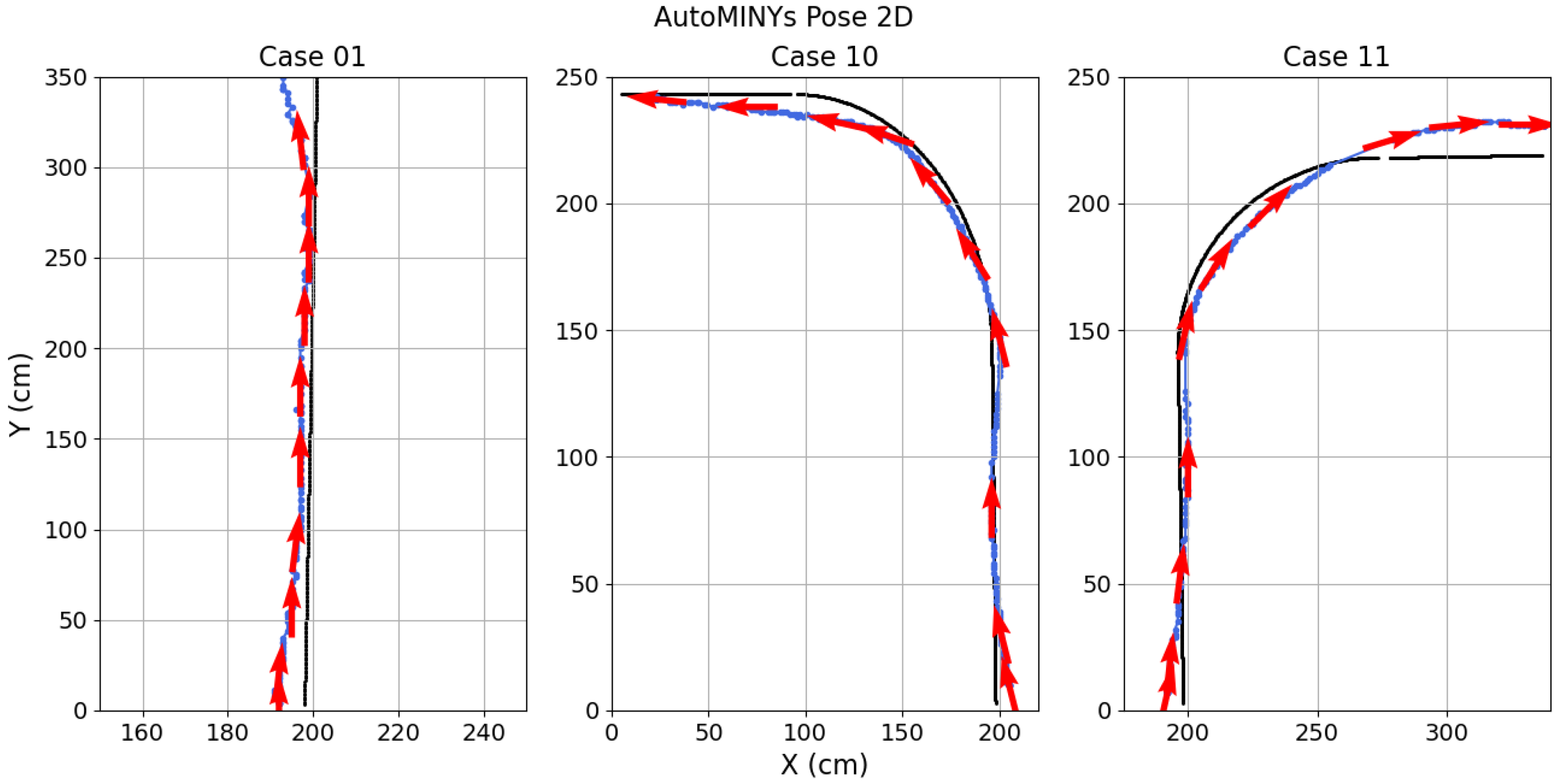
Figure 16 shows both the reference trajectory and the mean trajectory followed by the car during the 10 trials using the proposed controller (15), where it can be shown that the trajectories were tracked with a few centimeters error, which is acceptable for a prototype scaled vehicle. A video of the experiments is available at https://youtu.be/Tnf-_E8l6jo?si=pVEqnw_1i7ZdY6mW (accessed on 30 July 2025).

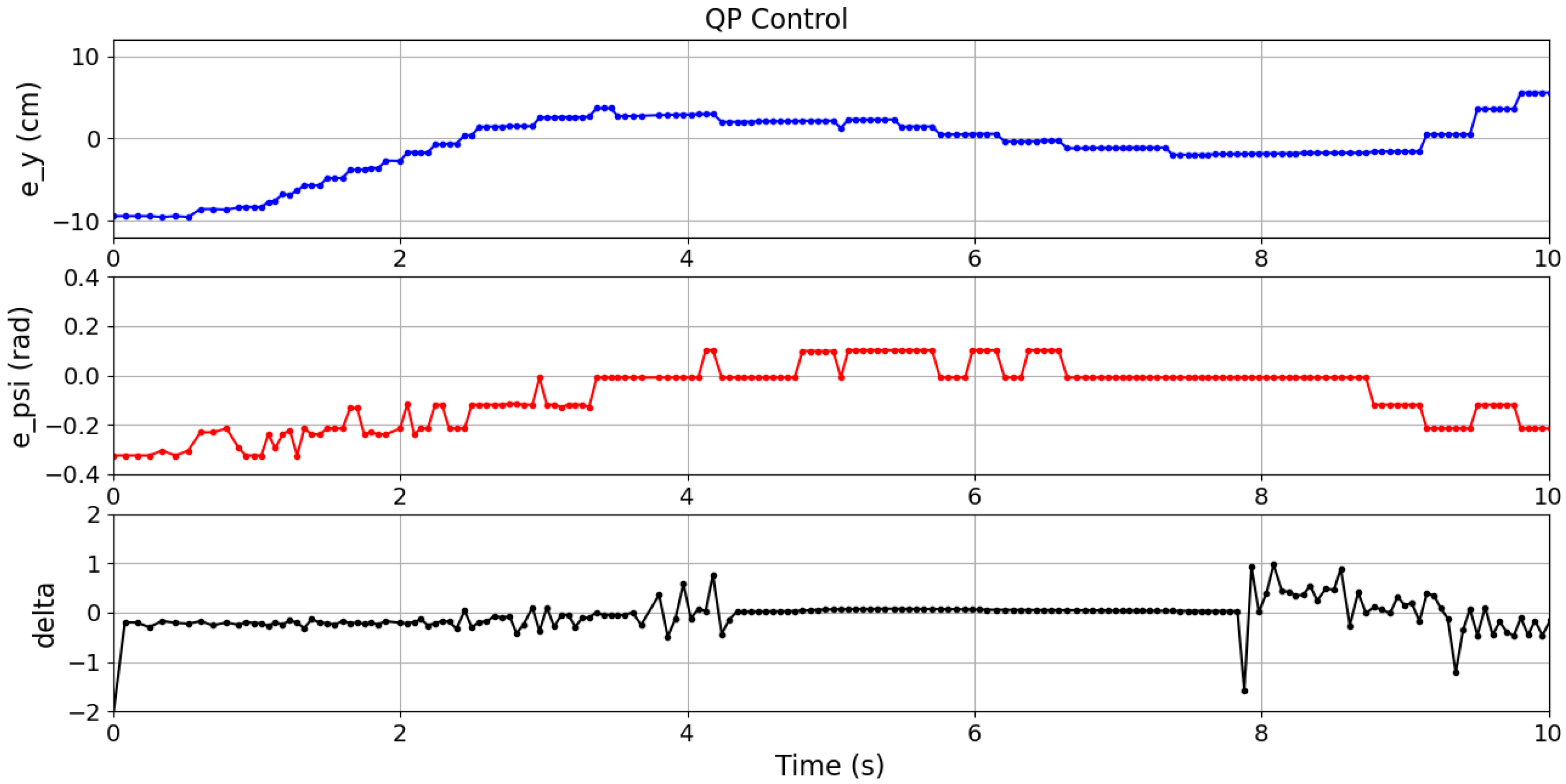
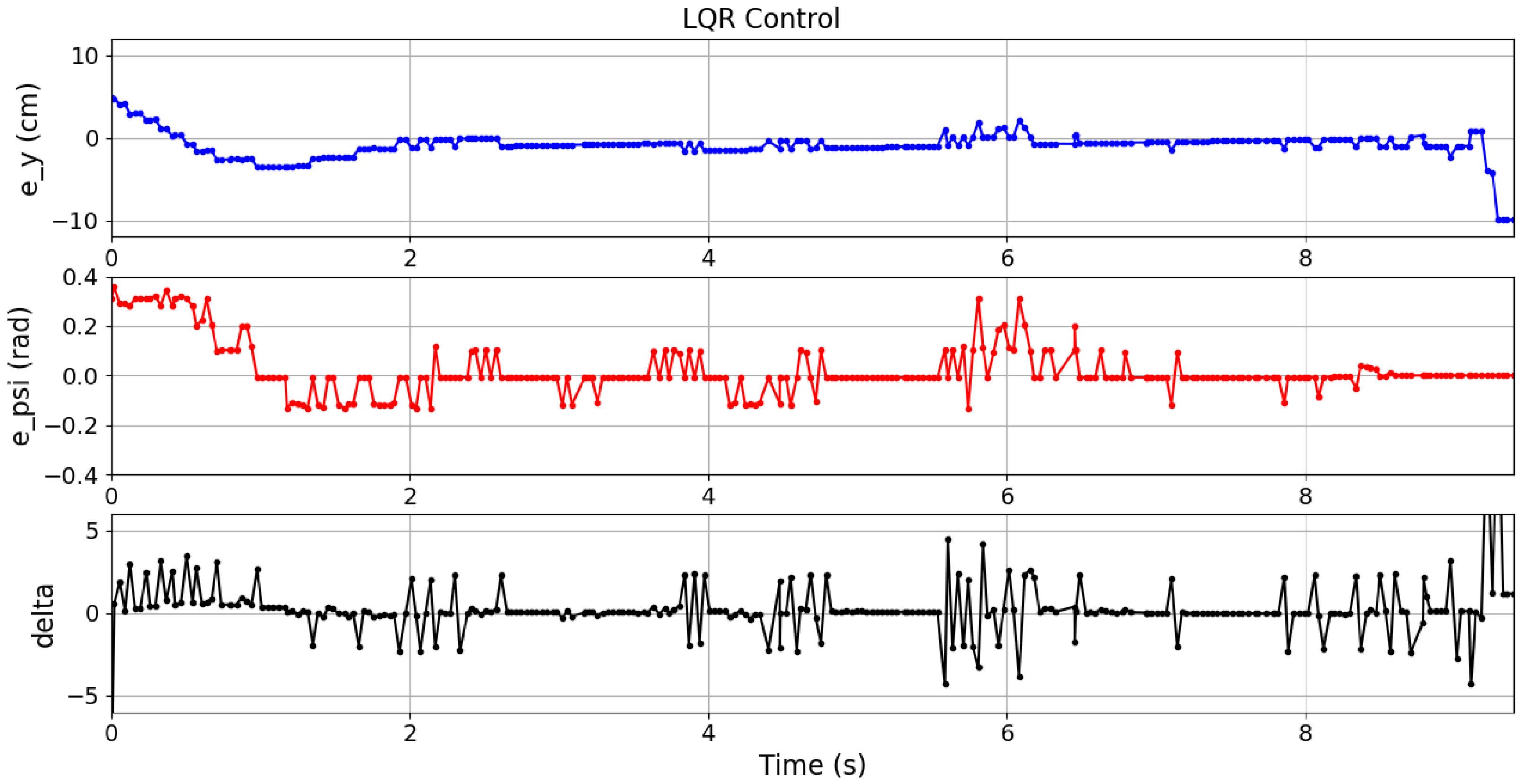
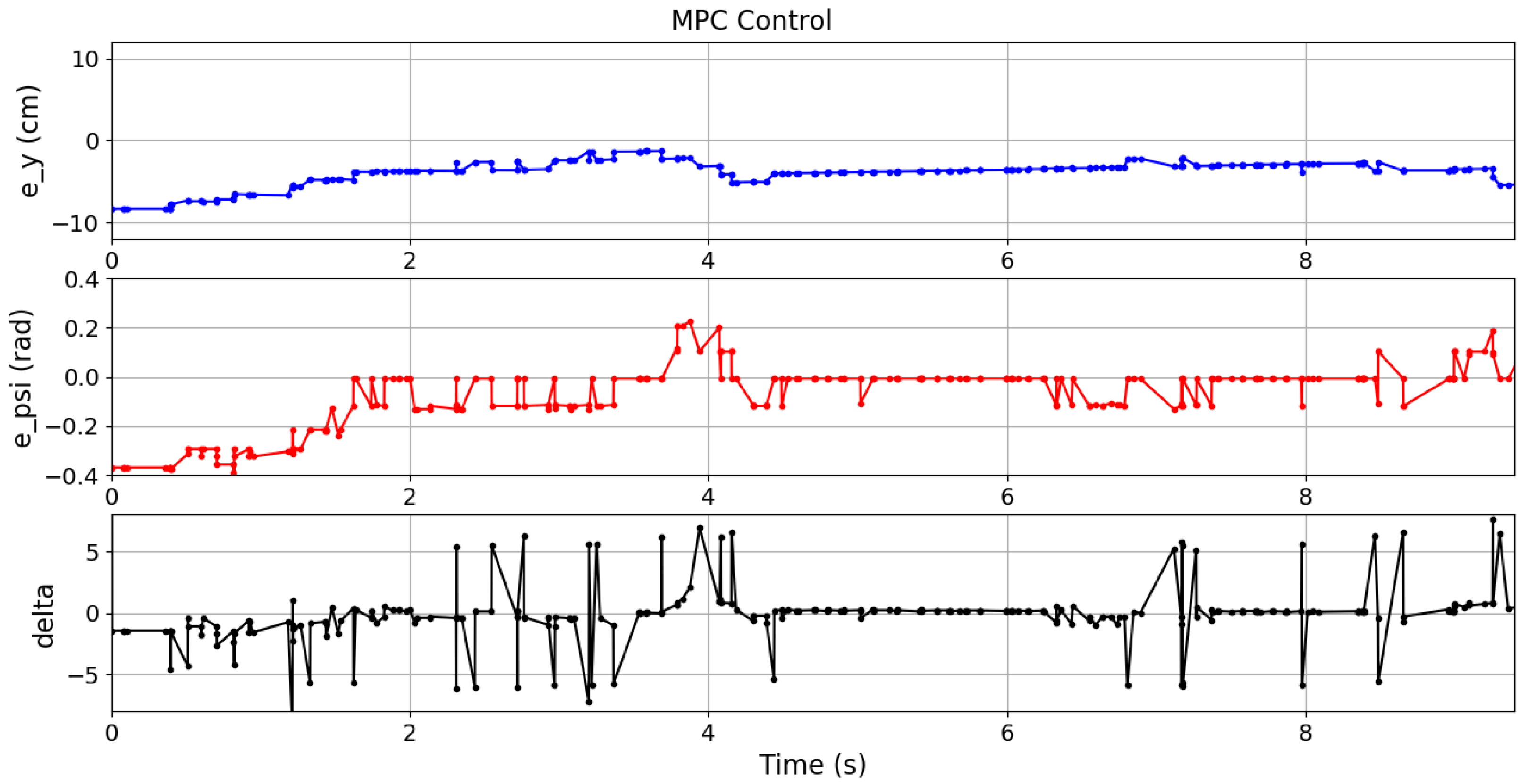
In order to compare the performance of this controller with other approaches, LQR and MPC controllers were also implemented to follow the ideal trajectory based on ground-truth information. As before, ten experiments were carried out for each case, the initial pose of the car was varied in each trial, and the RMSE of $e_y$, the ISE of $e_{\psi }$, and the TCE of $\delta$ were measured. It is worth mentioning that both LQR and MPC require the use of ground-truth data to be implemented; in contrast, QP control is exclusively fedback with the on-board sensors.

Table 3. RMSE, ISE, and TCE mean of the QP, LQR and MPC signals. The lowest values for each case are highlighted in bold.

Controller	Case	$\overline{\mathbf{RMSE}}{\mathit{e}}_{\mathit{y}}$	$\overline{\mathbf{ISE}}{\mathit{e}}_{\mathit{\psi }}$	${\overline{\mathbf{TCE}}}_{\mathit{\delta }}$
QP	01	6.0422	2.7277	2.4320
	10	10.0003	4.9394	8.2269
	11	9.2055	6.3084	6.9541
	Avg.	8.4160	4.6585	5.8710
LQR with GT	01	4.9287	8.5903	11.0374
	10	4.8819	13.6381	17.0680
	11	6.2626	20.1073	19.9529
	Avg.	5.3577	14.1119	16.0194
MPC with GT	01	7.6805	4.4789	20.5100
	10	6.8492	8.1341	29.4932
	11	6.3466	17.6865	31.4997
	Avg.	6.9588	10.0998	27.1676

reports the mean values of these metrics over ten experiments for each case. In these experiments, the vehicle navigated within an intersection, following the path of the case 01. The different controllers results are plotted as follows: QP control in Figure 17, LQR control in Figure 18, and MPC control in Figure 19.

Although the best $\overline{\mathrm{RMSE}}$$e_y$ was achieved by the LQR controller in all cases, it is important to note that the QP controller (15) obtained comparable results using only on-board information from the IMU and the camera, which demonstrates its superiority in more realistic sensing conditions. Moreover, the QP controller resulted in the lowest ISE and TCE across all cases. It can also be observed in Figure 17, Figure 18 and Figure 19 where the errors and control signals were plotted. It can be clearly observed that the control signal supplied by the QP control is effectively constrained within the desired range, and also smoother than those obtained through the other compared controllers, which may potentially contribute to improve the passenger comfort and increase the life cycle of actuators.

7. Conclusions

In this work, a Quadratic Programming (QP)-based controller was developed and evaluated for the autonomous navigation of a scale-size autonomous vehicle in intersection scenarios. The execution of the experiments was performed using computer vision techniques, namely the computation of the dynamic states by means of an homography-based estimation. Lane markings were also segmented, enabling accurate measurement of the vehicle’s lateral and heading errors.

A ground-truth system was implemented using a ceiling-mounted camera with colored markers, which proved to be highly useful for validating and quantifying the performance of the controllers. Additionally, a Convolutional Neural Network (CNN) was used to detect whether the vehicle was inside or outside an intersection with high accuracy, facilitating the correct switching between straight driving and intersection navigation controllers.

The proposed QP control was validated both mathematically via a Lyapunov method analysis and also experimentally in a real scale-model vehicle. The experimental results showed that the QP controller, which relied solely on on-board sensor information, achieved a competitive performance for lateral lane tracking compared to the LQR and MPC controllers that used ground-truth data. However, the proposed QP controller is significantly more accurate for curve tracking, demonstrating an average 67.0% lower ISE compared to the LQR and an average 53.9% lower ISE compared to the MPC. Moreover, when considering the TCE, the QP controller proved to be significantly more energy-efficient, reducing the required effort by an average of 63.3% compared to the LQR and by an average of 78.4% compared to the MPC, suggesting a less energy consumption and smoother operation, which can be potentially translated into a comfortable passenger experience, actuators preservation, and gentle maneuvers. In addition, it was proved that the control signals supplied by the QP control are correctly constrained to the selected range in contrast to the other compared techniques. These findings validate the feasibility of combining vision-based techniques with QP control for autonomous vehicle applications in controlled environments.

On the one hand, one potential limitation of the proposed controller is that it is designed to work efficiently in flat-surface navigation, so that roll and pitch motions can be negligible. On the other hand, the proposed model excels for scale-sized vehicles, but a more complex model must be implemented for real-sized ones.

As future work, the control system could be extended to more complex scenarios and include additional sensors to improve the controller’s robustness and adaptability. Additionally, the visual perception system can be improved by detecting the lanes and other signals trough semantic segmentation with CNN, which is beneficial to discard disturbing objects on the road, for instance, splashed liquids, garbage, or hail.

References

1. Bichiou, Y.; Rakha, H.A. Developing an optimal intersection control system for automated connected vehicles. IEEE Trans. Intell. Transp. Syst. 2018, 20, 1908–1916. [Google Scholar] [CrossRef]
2. Li, S.; Shu, K.; Chen, C.; Cao, D. Planning and decision-making for connected autonomous vehicles at road intersections: A review. Chin. J. Mech. Eng. 2021, 34, 133. [Google Scholar] [CrossRef]
3. Zhong, Z.; Nejad, M.; Lee, E.E. Autonomous and semiautonomous intersection management: A survey. IEEE Intell. Transp. Syst. Mag. 2020, 13, 53–70. [Google Scholar] [CrossRef]
4. Bouyarmane, K.; Chappellet, K.; Vaillant, J.; Kheddar, A. Quadratic programming for multirobot and task-space force control. IEEE Trans. Robot. 2018, 35, 64–77. [Google Scholar] [CrossRef]
5. Alonso, J.; Milanés, V.; Pérez, J.; Onieva, E.; González, C.; de Pedro, T. Autonomous vehicle control systems for safe crossroads. Transp. Res. Part C Emerg. Technol. 2011, 19, 1095–1110. [Google Scholar] [CrossRef]
6. Riegger, L.; Carlander, M.; Lidander, N.; Murgovski, N.; Sjöberg, J. Centralized MPC for Autonomous Intersection Crossing. In Proceedings of the 2016 IEEE 19th International Conference on Intelligent Transportation Systems (ITSC), Rio de Janeiro, Brazil, 1–4 November 2016; pp. 1372–1377. [Google Scholar] [CrossRef]
7. Meng, X.; Cassandras, C.G. Optimal Control of Autonomous Vehicles for Non-Stop Signalized Intersection Crossing. In Proceedings of the 2018 IEEE Conference on Decision and Control (CDC), Miami, FL, USA, 17–19 December 2018; pp. 6988–6993. [Google Scholar] [CrossRef]
8. Ding, Z.; Sun, C.; Zhou, M.; Liu, Z.; Wu, C. Intersection vehicle turning control for fully autonomous driving scenarios. Sensors 2021, 21, 3995. [Google Scholar] [CrossRef] [PubMed]
9. Vitale, C.; Kolios, P.; Ellinas, G. Autonomous intersection crossing with vehicle location uncertainty. IEEE Trans. Intell. Transp. Syst. 2022, 23, 17546–17561. [Google Scholar] [CrossRef]
10. Morimoto, E.; Suguri, M.; Umeda, M. Vision-based Navigation System for Autonomous Transportation Vehicle. Precis. Agric. 2005, 6, 239–254. [Google Scholar] [CrossRef]
11. Sezer, V.; Bandyopadhyay, T.; Rus, D.; Frazzoli, E.; Hsu, D. Towards autonomous navigation of unsignalized intersections under uncertainty of human driver intent. In Proceedings of the 2015 IEEE/RSJ International Conference on Intelligent Robots and Systems (IROS), Hamburg, Germany, 28 September–2 October 2015; pp. 3578–3585. [Google Scholar] [CrossRef]
12. Barrera-Ramírez, C.; González-Miranda, O.; Ibarra-Zannatha, J.M. Sistema de planeación y control de navegación para un vehículo autónomo en un entorno urbano. Pädi Boletín Científico de Ciencias Básicas e Ingenierías del ICBI 2022, 10, 27–35. [Google Scholar] [CrossRef]
13. Pourjafari, N.; Ghafari, A.; Ghaffari, A. Navigating unsignalized intersections: A predictive approach for safe and cautious autonomous driving. IEEE Trans. Intell. Veh. 2023, 9, 269–278. [Google Scholar] [CrossRef]
14. Zannatha, J.M.I.; Miranda, O.G.; Ramírez, C.B.; Miranda, L.A.L.; Aguilar, S.R.A.; Osuna, L.Á.D. Integration of perception, planning and control in the autominy 4.0. In Proceedings of the 2022 19th International Conference on Electrical Engineering, Computing Science and Automatic Control (CCE), Mexico City, Mexico, 9–11 November 2022; pp. 1–6. [Google Scholar] [CrossRef]
15. Alcalá, E.; Puig, V.; Quevedo, J.; Escobet, T.; Comasolivas, R. Autonomous vehicle control using a kinematic Lyapunov-based technique with LQR-LMI tuning. Control Eng. Pract. 2018, 73, 1–12. [Google Scholar] [CrossRef]
16. Hu, J.; Xiong, S.; Zha, J.; Fu, C. Lane Detection and Trajectory Tracking Control of Autonomous Vehicle Based on Model Predictive Control. Int. J. Automot. Technol. 2020, 21, 285–295. [Google Scholar] [CrossRef]
17. Yuan, T.; Zhao, R. LQR-MPC-Based Trajectory-Tracking Controller of Autonomous Vehicle Subject to Coupling Effects and Driving State Uncertainties. Sensors 2022, 22, 5556. [Google Scholar] [CrossRef] [PubMed]
18. Bousskoul, A.E.; Ouachtouk, I.; Ait Elmahjoub, A. Path Tracking for Self-driving Cars: Stanley and LQR Controllers Comparison. In Innovative Technologies on Electrical Power Systems for Smart Cities Infrastructure (ICESST), Proceedings of the 1st International Conference on Electrical Systems and Smart Technologies, Dakhla, Morocco, 11–13 December 2024; Sustainable Civil Infrastructures; Springer: Cham, Switzerland, 2025; pp. 337–346. [Google Scholar] [CrossRef]
19. Lee, D.H. Lane-Keeping Control of Autonomous Vehicles Through a Soft-Constrained Iterative LQR. IEEE Trans. Veh. Technol. 2025, 74, 5610–5623. [Google Scholar] [CrossRef]
20. Rajamani, R. Vehicle Dynamics and Control; Springer Science & Business Media: Berlin/Heidelberg, Germany, 2011. [Google Scholar]
21. Kulkarni, A.J. Optimization Methods and Algorithms; Springer: Singapore, 2025. [Google Scholar]
22. Hao, T.; Wen, J.; Xiong, J. Maximum Principle of Stochastic Optimal Control Problems with Model Uncertainty. J. Optim. Theory Appl. 2025, 207, 27. [Google Scholar] [CrossRef]
23. Abdalla, M.; Alsafartee, J.H. Optimized Model Reduction Using Reducibility Matrix. In Proceedings of the 2025 5th International Conference on Artificial Intelligence and Industrial Technology Applications (AIITA), Xi’an, China, 28–30 March 2025; pp. 1285–1289. [Google Scholar]
Figure 1. Diagram of parameters involved in the simplified vehicle model. Red and Blue arrows denote the vehicle’s reference frame axes.
Actuators 14 00494 g001
Figure 2. Assembled AutoMINY platform.
Actuators 14 00494 g002
Figure 3. AutoMINY with labeled components including sensors, actuators, and on-board computer.
Actuators 14 00494 g003
Figure 4. System diagram of the AutoMINY platform. Red arrows indicate power connections (5 V and 14.8 V); blue arrows represent USB communication links; black arrows denote other connections between components.
Actuators 14 00494 g004
Figure 5. ROS-based modular architecture using LQR or MPC control.
Actuators 14 00494 g005
Figure 6. ROS-based modular architecture using QP control.
Actuators 14 00494 g006
Figure 7. Perspective correction of the road. (a) Initial RGB image of the road. The orange lines are the road signs. The yellow line is a part of the experimental setup used for other works regardless this paper. (b) Color segmentation. (c) Homography of the road.
Actuators 14 00494 g007
Figure 8. Processing pipeline of the ground-truth system. The pipeline includes image acquisition from a ceiling-mounted fisheye camera, distortion correction, homography transformation to obtain a bird’s-eye view, color segmentation for marker detection, and pose estimation using image moments.
Actuators 14 00494 g008
Figure 9. Visual localization of the vehicle using colored markers. Left: image of the physical scene showing the top of the vehicle with green and blue markers. Right: top-down view obtained through homography, enabling precise estimation of vehicle position and orientation.
Actuators 14 00494 g009
Figure 10. Architecture of the CNN.
Actuators 14 00494 g010
Figure 11. Examples from the dataset used to train the CNN. The first row corresponds to the Out class, and the second to the In class.
Actuators 14 00494 g011
Figure 12. Confusion matrix for the validation of a 313 images dataset. The network classifies images with an accuracy of 97.9% , since 303 were correctly classified and 10 missclassified for the OUT class, while 312 were correctly classified and 1 missclassified for the case of the IN class.
Actuators 14 00494 g012
Figure 13. Measurement of the states e y and e ψ using the homography of the road. The heading error e ψ is defined as the angle between the secant line of the right lane marking (in green) and the optical axis (in blue). The lateral error is given by e y = y 1 y r e f .
Actuators 14 00494 g013
Figure 14. Shape of the function ζ k defined as the difference between two sigmoid curves. This function creates a smooth transition between controllers over time.
Actuators 14 00494 g014
Figure 15. Two controllers were used during navigation: a vision-based controller for lane keeping (in blue), and an IMU-based controller for navigating the cruise section (in green). The three possible paths were labeled as 01, 10, and 11.
Actuators 14 00494 g015
Figure 16. The trajectory of the car measured by the Ground-Truth system. Each path was labeled as 01, 10, and 11. Black line is the desired trajectory. Blue line is the average of performed trajectories. Red arrows denote the orientation of the car and the sense of the motion.
Actuators 14 00494 g016
Figure 17. Time evolution of the lateral error e y (blue), heading error e ψ (red), and steering angle δ (black) during intersection navigation using the proposed QP-based control strategy.
Actuators 14 00494 g017
Figure 18. Time evolution of the lateral error e y (blue), heading error e ψ (red), and steering angle δ (black) during intersection navigation using the LQR control strategy.
Actuators 14 00494 g018
Figure 19. Time evolution of the lateral error e y (blue), heading error e ψ (red), and steering angle δ (black) during intersection navigation using the MPC strategy.
Actuators 14 00494 g019