

Physics-Informed Neural Network-Based Input Shaping for Vibration Suppression of Flexible Single-Link Robots


Abstract
1. Introduction
- 1.
- Network learning for input shaping: The proposed method leverages efficient neural network techniques and its powerful computational resources to search for optimal input shapers for vibration suppression, with results that outperform conventional methods in complex motion scenarios.
- 2.
- Multimode vibration suppression: The proposed method enhances the effectiveness of vibration suppression by utilizing a larger number of modes, while its computational burden remains manageable as the number of modes increases.
- 3.
- Direct feed-forward control design: The optimal impulse sequence and network output can be used directly in feed-forward control algorithms, eliminating the need to solve the system.
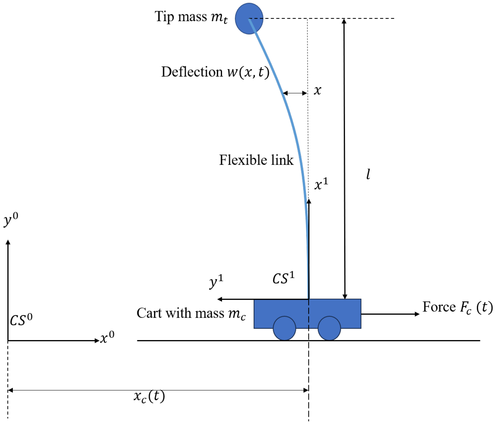
2. Problem Formulation
3. PINN-Based Input-Shaping Method
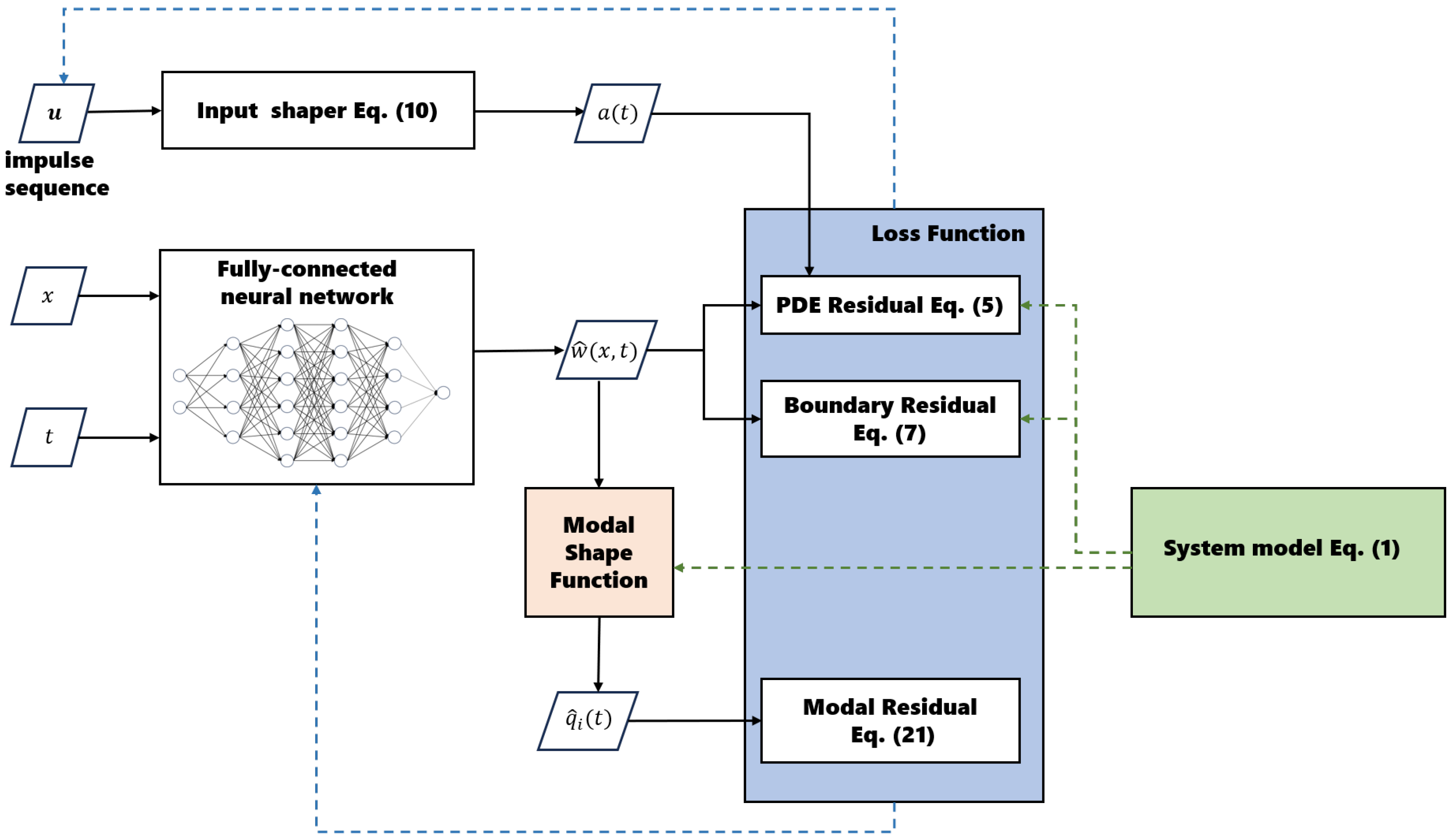
3.1. PINN Structure
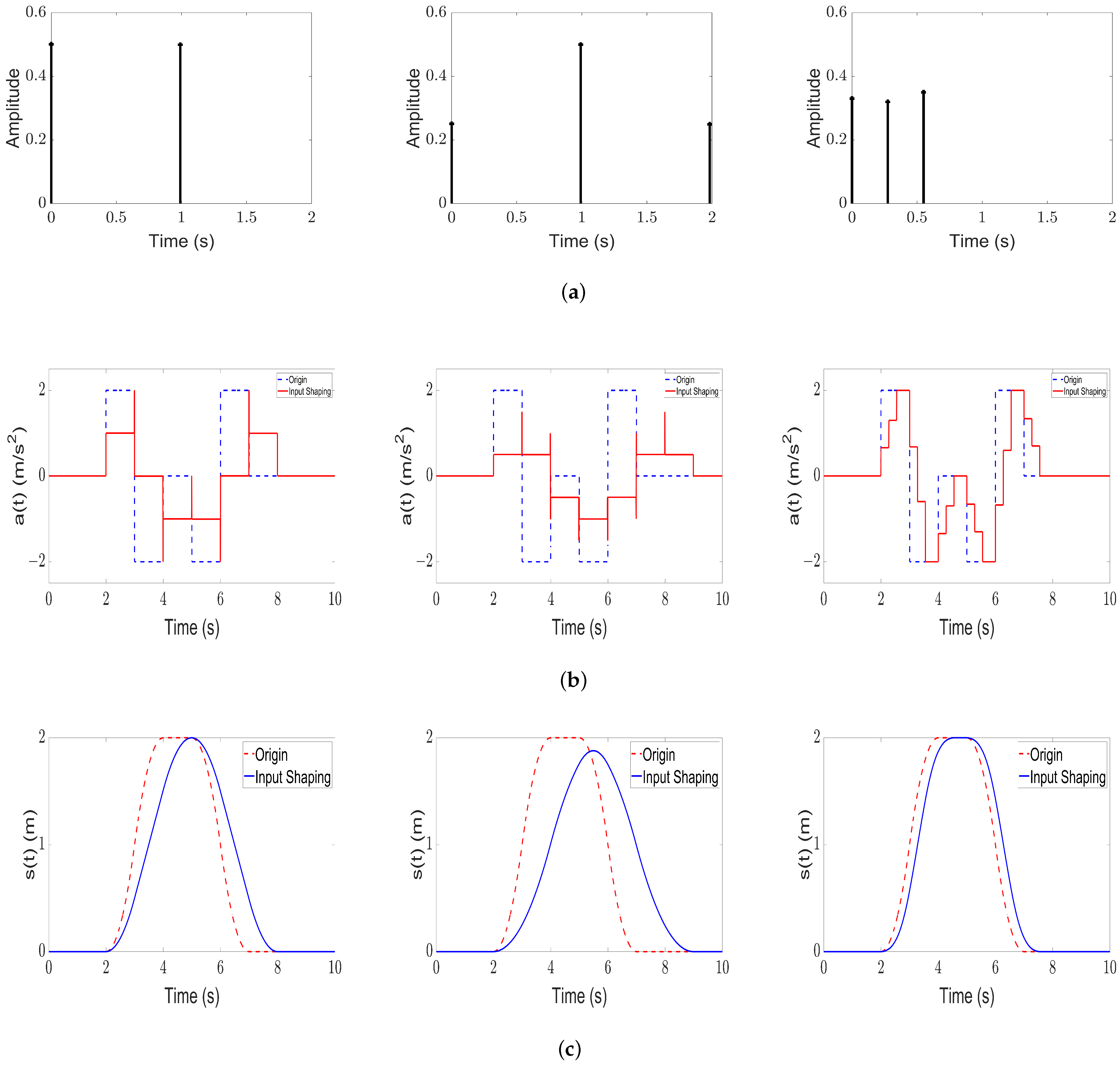
3.2. Input-Shaping Technique
3.2.1. ZV Shaper
3.2.2. ZVD Shaper
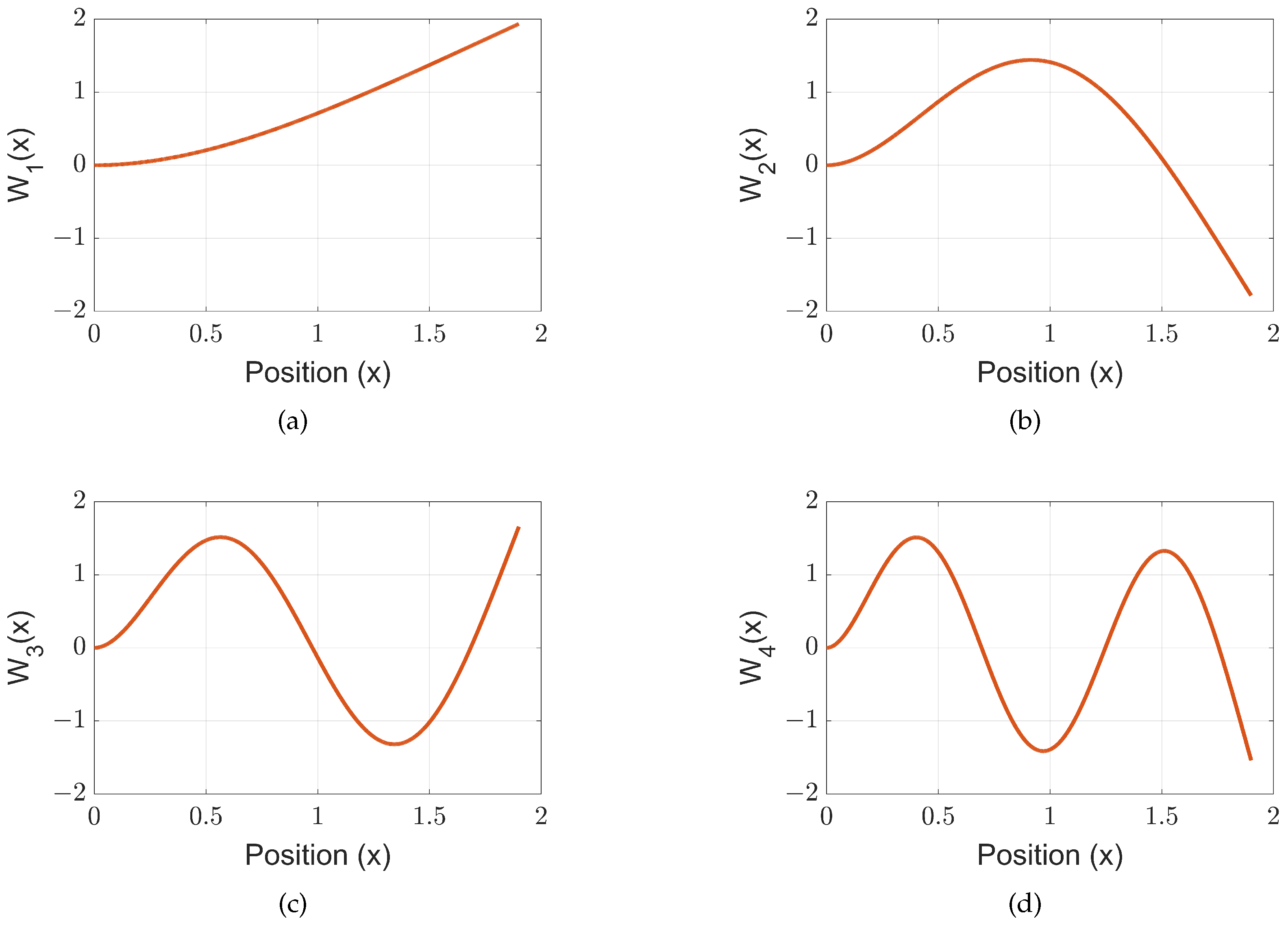
3.3. Modal-Based Loss Function
3.4. Two-Phase Training
- 1.
- Coarse-Tuning Phase: Network Parameter SelectionIn the coarse-tuning phase, we focus on determining the network parameters for the flexible system represented by PDEs. During this phase, only the physical model constraints are considered.In this phase, the impulse command, , is given and fixed. Starting from the randomly initialized network parameters, , we employ gradient-based optimization to find an optimal set of values, , that minimize the system model loss function, . During each iteration k, the parameters are updated as follows:To enhance training efficiency and convergence, a StepLR learning rate scheduler is employed. This scheduler decays the learning rate by a factor of every s epochs, following the rulewhere is the initial learning rate and s denotes the number of epochs after which the learning rate is decayed by a factor of .These learned network parameters are crucial for effectively addressing the dynamics of the PDEs and serve as a foundation for subsequent vibration suppression optimization.
- 2.
- Fine-Tuning Phase: Learning Optimal Impulse CommandIn the second phase, we utilize the established network structure, , with the learned network parameters and enhance it by introducing input-shaping commands, , as trainable parameters within the neural network. This phase involves minimizing a composite loss function, , which consists of both the system model residuals and additional vibration modal residuals.The weights, , in the compound loss function, , are adjusted to prioritize the vibration suppression performance. The exact values of these weights are chosen based on observations from initial training runs, aiming to minimize residual vibrations as effectively as possible while maintaining model accuracy (i.e., ensuring the model constraints are satisfied). In this fine-tuning phase, the network parameters, , are initialized to the optimal values, , obtained in the first phase, and the impulse command, , is initialized to the values used in the first phase. They are updated simultaneously according to the following rule:The learning rate, , decays according to the same rule as described in Equation (26).Ultimately, the training yields an optimized control solution, , and a corresponding improved system response, , with network parameters , thus achieving an effective balance between accurately modeling system dynamics and mitigating undesirable vibrations.
4. Feed-Forward Control
5. Simulation Results
5.1. Input Shaping on Single Mode
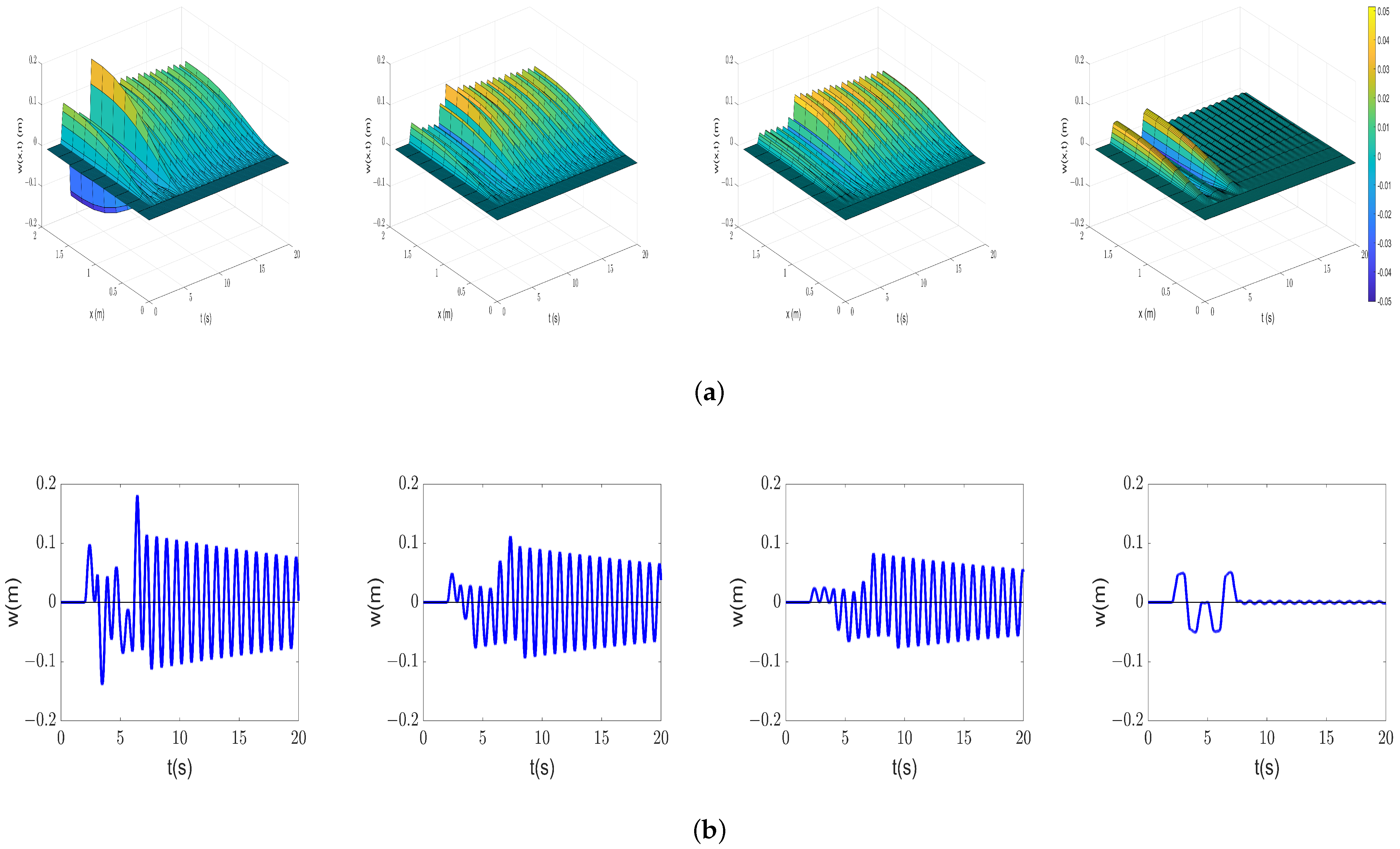
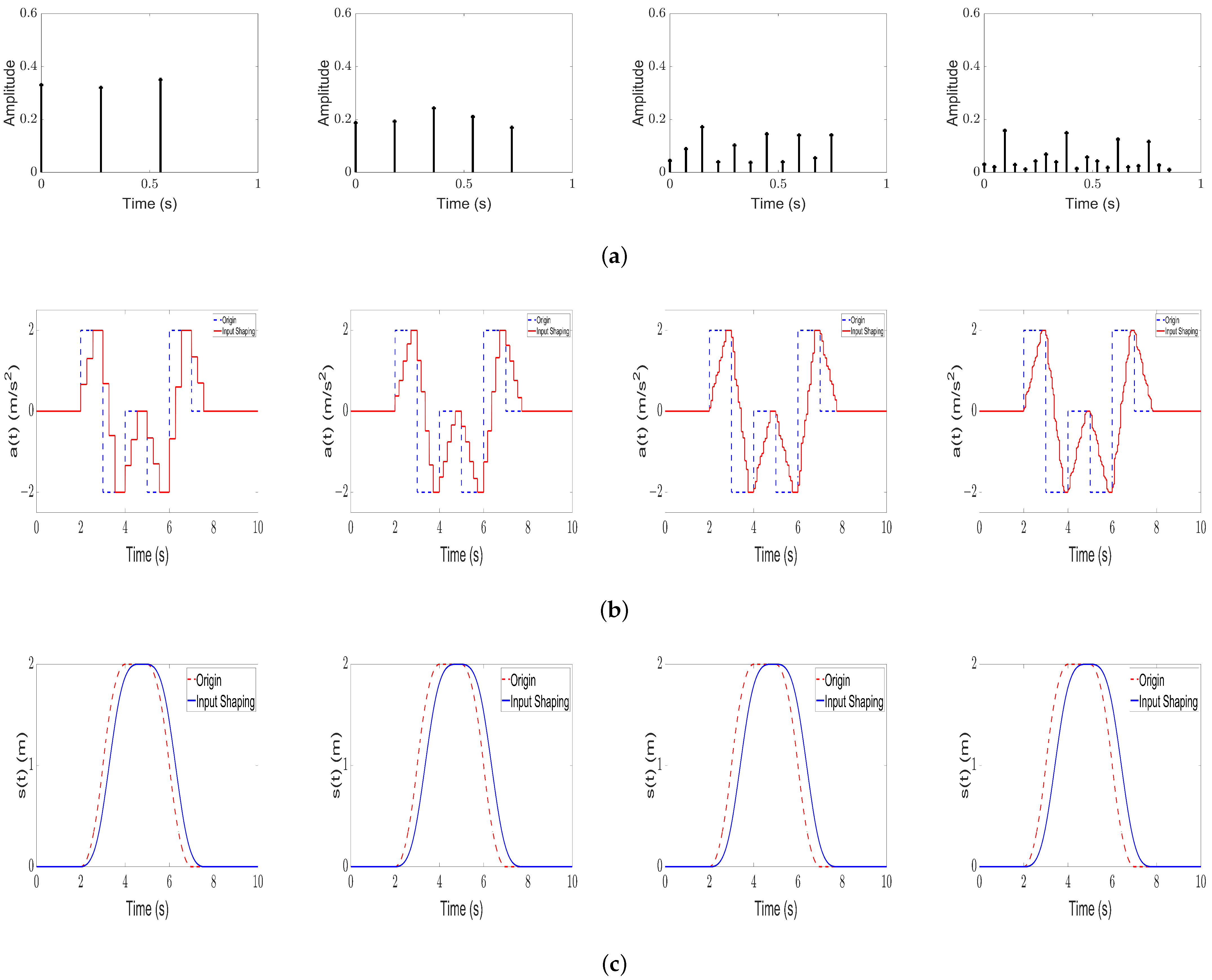
5.2. Input Shaping on Multiple Modes
5.3. Feed-Forward Controller Design
6. Conclusions
Author Contributions
Funding
Data Availability Statement
Conflicts of Interest
References
- Patidar, V.; Tiwari, R. Survey of robotic arm and parameters. In Proceedings of the 2016 International Conference on Computer Communication and Informatics (ICCCI), Coimbatore, India, 7–9 January 2016; IEEE: Piscataway, NJ, USA, 2016; pp. 1–6. [Google Scholar]
- Kanoh, H.; Tzafestas, S.; Lee, H.G.; Kalat, J. Modelling and control of flexible robot arms. In Proceedings of the 1986 25th IEEE Conference on Decision and Control, Athens, Greece, 10–12 December 1986; IEEE: Piscataway, NJ, USA, 1986; pp. 1866–1870. [Google Scholar]
- Turner, J.D.; Chun, H.M. Optimal distributed control of a flexible spacecraft during a large-angle maneuver. J. Guid. Control Dyn. 1984, 7, 257–264. [Google Scholar] [CrossRef]
- Churr, H.M.; Turner, J.D.; Juang, J.N. Disturbance-accommodating tracking maneuvers of flexible spacecraft. J. Astronaut. Sci. 1985, 33, 197–216. [Google Scholar]
- Kim, J.; de Mathelin, M.; Ikuta, K.; Kwon, D.S. Advancement of flexible robot technologies for endoluminal surgeries. Proc. IEEE 2022, 110, 909–931. [Google Scholar] [CrossRef]
- Omisore, O.M.; Han, S.; Xiong, J.; Li, H.; Li, Z.; Wang, L. A review on flexible robotic systems for minimally invasive surgery. IEEE Trans. Syst. Man Cybern. Syst. 2020, 52, 631–644. [Google Scholar] [CrossRef]
- Müller, P.A.; Liu, S. Vibration control of a flexible single-link robot: A backstepping controller for distributed parameter systems. In Proceedings of the IECON 2014-40th Annual Conference of the IEEE Industrial Electronics Society, Dallas, TX, USA, 29 October–1 November 2014; IEEE: Piscataway, NJ, USA, 2014; pp. 2890–2896. [Google Scholar]
- Benosman, M.; Le Vey, G. Control of flexible manipulators: A survey. Robotica 2004, 22, 533–545. [Google Scholar] [CrossRef]
- Kiang, C.T.; Spowage, A.; Yoong, C.K. Review of control and sensor system of flexible manipulator. J. Intell. Robot. Syst. 2015, 77, 187–213. [Google Scholar] [CrossRef]
- Garcia-Perez, O.; Silva-Navarro, G.; Peza-Solis, J. Flexible-link robots with combined trajectory tracking and vibration control. Appl. Math. Model. 2019, 70, 285–298. [Google Scholar] [CrossRef]
- Ghasemi, A.H. Slewing and vibration control of a single-link flexible manipulator using filtered feedback linearization. J. Intell. Mater. Syst. Struct. 2017, 28, 2887–2895. [Google Scholar] [CrossRef]
- Sun, C.; Gao, H.; He, W.; Yu, Y. Fuzzy neural network control of a flexible robotic manipulator using assumed mode method. IEEE Trans. Neural Netw. Learn. Syst. 2018, 29, 5214–5227. [Google Scholar] [CrossRef] [PubMed]
- Ouyang, Y.; He, W.; Li, X.; Liu, J.K.; Li, G. Vibration Control Based on Reinforcement Learning for a Single-link Flexible Robotic Manipulator. IFAC-PapersOnLine 2017, 50, 3476–3481. [Google Scholar] [CrossRef]
- Hyde, J.M.; Seering, W.P. Using Input Command Pre-Shaping to Suppress Multiple Mode Vibration; MIT Space Engineering Research Center: Cambridge, MA, USA, 1990. [Google Scholar]
- Singhose, W.E.; Seering, W.P.; Singer, N.C. Shaping inputs to reduce vibration: A vector diagram approach. In Proceedings of the IEEE International Conference on Robotics and Automation, Cincinnati, OH, USA, 13–18 May 1990; IEEE: Piscataway, NJ, USA, 1990; pp. 922–927. [Google Scholar]
- ur Rehman, S.F.; Mohamed, Z.; Husain, A.R.; Jaafar, H.I.; Shaheed, M.H.; Abbasi, M.A. Input shaping with an adaptive scheme for swing control of an underactuated tower crane under payload hoisting and mass variations. Mech. Syst. Signal Process. 2022, 175, 109106. [Google Scholar] [CrossRef]
- Maghsoudi, M.J.; Mohamed, Z.; Husain, A.; Tokhi, M. An optimal performance control scheme for a 3D crane. Mech. Syst. Signal Process. 2016, 66, 756–768. [Google Scholar] [CrossRef]
- Maghsoudi, M.J.; Mohamed, Z.; Sudin, S.; Buyamin, S.; Jaafar, H.; Ahmad, S. An improved input shaping design for an efficient sway control of a nonlinear 3D overhead crane with friction. Mech. Syst. Signal Process. 2017, 92, 364–378. [Google Scholar] [CrossRef]
- Masoud, Z.N.; Alhazza, K.A. Frequency-modulation input shaping control of double-pendulum overhead cranes. J. Dyn. Syst. Meas. Control 2014, 136, 021005. [Google Scholar] [CrossRef]
- Thomsen, D.K.; Søe-Knudsen, R.; Balling, O.; Zhang, X. Vibration control of industrial robot arms by multi-mode time-varying input shaping. Mech. Mach. Theory 2021, 155, 104072. [Google Scholar] [CrossRef]
- Mishra, A.; Yau, H.T.; Kuo, P.H.; Wang, C.C. Achieving sustainability by identifying the influences of cutting parameters on the carbon emissions of a milling process. Int. J. Adv. Manuf. Technol. 2024, 135, 5409–5427. [Google Scholar] [CrossRef]
- Peng, T.J.; Kuo, P.H.; Huang, W.C.; Wang, C.C. Nonlinear Dynamic Analysis and Forecasting of Symmetric Aerostatic Cavities Bearing Systems. Int. J. Bifurc. Chaos 2024, 34, 2430008. [Google Scholar] [CrossRef]
- Abdulrahman, S.M.; Asaad, R.R.; Ahmad, H.B.; Hani, A.A.; Zeebaree, S.R.; Sallow, A.B. Machine Learning in Nonlinear Material Physics. J. Soft Comput. Data Min. 2024, 5, 122–131. [Google Scholar] [CrossRef]
- Hu, C.; Wu, Z. Model predictive control of switched nonlinear systems using online machine learning. Chem. Eng. Res. Des. 2024, 209, 221–236. [Google Scholar] [CrossRef]
- Raissi, M.; Perdikaris, P.; Karniadakis, G.E. Physics-informed neural networks: A deep learning framework for solving forward and inverse problems involving nonlinear partial differential equations. J. Comput. Phys. 2019, 378, 686–707. [Google Scholar] [CrossRef]
- Pang, G.; Lu, L.; Karniadakis, G.E. fPINNs: Fractional physics-informed neural networks. SIAM J. Sci. Comput. 2019, 41, A2603–A2626. [Google Scholar] [CrossRef]
- Li, Z.; Kovachki, N.; Azizzadenesheli, K.; Liu, B.; Bhattacharya, K.; Stuart, A.; Anandkumar, A. Fourier neural operator for parametric partial differential equations. arXiv 2020, arXiv:2010.08895. [Google Scholar]
- Chen, Y.; Koohy, S. Gpt-pinn: Generative pre-trained physics-informed neural networks toward non-intrusive meta-learning of parametric pdes. Finite Elem. Anal. Des. 2024, 228, 104047. [Google Scholar] [CrossRef]
- Wang, Y.; Zhong, L. NAS-PINN: Neural architecture search-guided physics-informed neural network for solving PDEs. J. Comput. Phys. 2024, 496, 112603. [Google Scholar] [CrossRef]
- Bai, J.; Rabczuk, T.; Gupta, A.; Alzubaidi, L.; Gu, Y. A physics-informed neural network technique based on a modified loss function for computational 2D and 3D solid mechanics. Comput. Mech. 2023, 71, 543–562. [Google Scholar] [CrossRef]
- Luo, D.; Cai, Z.; Jiang, D.; Peng, H. Research on Parameter Identification Method for Robotic Manipulators Joint Friction Model Based on PINN. In Proceedings of the 2024 IEEE International Conference on Advanced Intelligent Mechatronics (AIM), Boston, MA, USA, 15–18 July 2024; IEEE: Piscataway, NJ, USA, 2024; pp. 948–953. [Google Scholar]
- Yang, X.; Du, Y.; Li, L.; Zhou, Z.; Zhang, X. Physics-Informed Neural Network for Model Prediction and Dynamics Parameter Identification of Collaborative Robot Joints. IEEE Robot. Autom. Lett. 2023, 8, 8462–8469. [Google Scholar] [CrossRef]
- Li, W.; Lee, K.M. Physics informed neural network for parameter identification and boundary force estimation of compliant and biomechanical systems. Int. J. Intell. Robot. Appl. 2021, 5, 313–325. [Google Scholar] [CrossRef]
- Nicodemus, J.; Kneifl, J.; Fehr, J.; Unger, B. Physics-informed neural networks-based model predictive control for multi-link manipulators. IFAC-PapersOnLine 2022, 55, 331–336. [Google Scholar] [CrossRef]


| Solution Type | Max Residual Vibration (m) | Total Residual Vibration () |
|---|---|---|
| No Input Shaping | 0.1116 | 1140.9643 |
| ZV | 0.0948 | 669.7387 |
| ZVD | 0.0823 | 537.7970 |
| PINN Solution (First Mode) | 0.0027 | 17.9913 |
| Solution Type | Modal Loss of the First Mode |
|---|---|
| ZV | 23.671 |
| ZVD | 23.374 |
| PINN Solution (First Mode) | 23.672 |
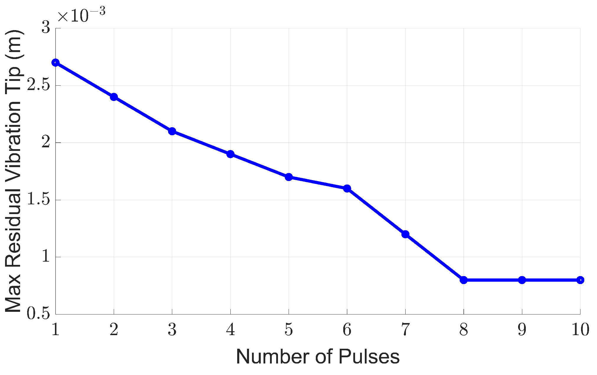
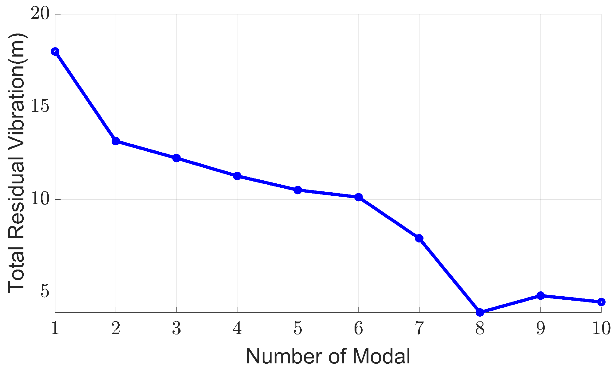
| Mode Number | Max Residual Vibration (m) | Total Residual Vibration () |
|---|---|---|
| 1 | 0.0027 | 17.9913 |
| 2 | 0.0024 | 13.1539 |
| 3 | 0.0021 | 12.2409 |
| 4 | 0.0019 | 11.2738 |
| 5 | 0.0017 | 10.5147 |
| 6 | 0.0016 | 10.1308 |
| 7 | 0.0012 | 7.9086 |
| 8 | 0.0008 | 3.9130 |
| 9 | 0.0008 | 4.8193 |
| 10 | 0.0008 | 4.4773 |
Disclaimer/Publisher’s Note: The statements, opinions and data contained in all publications are solely those of the individual author(s) and contributor(s) and not of MDPI and/or the editor(s). MDPI and/or the editor(s) disclaim responsibility for any injury to people or property resulting from any ideas, methods, instructions or products referred to in the content. |
© 2025 by the authors. Licensee MDPI, Basel, Switzerland. This article is an open access article distributed under the terms and conditions of the Creative Commons Attribution (CC BY) license (https://creativecommons.org/licenses/by/4.0/).
Share and Cite
Li, T.; Xiao, T. Physics-Informed Neural Network-Based Input Shaping for Vibration Suppression of Flexible Single-Link Robots. Actuators 2025, 14, 14. https://doi.org/10.3390/act14010014
Li T, Xiao T. Physics-Informed Neural Network-Based Input Shaping for Vibration Suppression of Flexible Single-Link Robots. Actuators. 2025; 14(1):14. https://doi.org/10.3390/act14010014
Chicago/Turabian StyleLi, Tingfeng, and Tengfei Xiao. 2025. "Physics-Informed Neural Network-Based Input Shaping for Vibration Suppression of Flexible Single-Link Robots" Actuators 14, no. 1: 14. https://doi.org/10.3390/act14010014
APA StyleLi, T., & Xiao, T. (2025). Physics-Informed Neural Network-Based Input Shaping for Vibration Suppression of Flexible Single-Link Robots. Actuators, 14(1), 14. https://doi.org/10.3390/act14010014