Path Planning for Wall-Climbing Robots Using an Improved Sparrow Search Algorithm

Abstract

Traditional path planning algorithms typically focus only on path length, which fails to meet the low energy consumption requirements for wall-climbing robots in bridge inspection. This paper proposes an improved sparrow search algorithm based on logistic–tent chaotic mapping and differential evolution, aimed at addressing the issue of the sparrow search algorithm’s tendency to fall into local optima, thereby optimizing path planning for bridge inspection. First, the initial population is optimized using logistic–tent chaotic mapping and refracted opposition-based learning, with dynamic adjustments to the population size during the iterative process. Second, improvements are made to the position updating formulas of both discoverers and followers. Finally, the differential evolution algorithm is introduced to enhance the global search capability of the algorithm, thereby reducing the robot’s energy consumption. Benchmark function tests verify that the proposed algorithm exhibits superior optimization capabilities. Further path planning simulation experiments demonstrate the algorithm’s effectiveness, with the planned paths not only consuming less energy but also exhibiting shorter path lengths, fewer turns, and smaller steering angles.

1. Introduction

As bridge infrastructure ages, traditional inspection methods like visual inspection and inspection vehicles have become increasingly inadequate. These methods are time-consuming and costly and pose safety risks, making them insufficient for efficient and precise assessments. In recent years, new technologies such as drones and LiDAR have emerged in bridge inspection. However, these methods still face challenges like blind spots and complex equipment. In contrast, wall-climbing robots [1] are gaining attention as an innovative solution. They offer advantages in flexibility, coverage, and safety. These robots can maneuver across various surfaces, including horizontal ground, vertical walls, and ceilings. They can replace humans in hazardous environments to perform high-risk tasks [2,3,4,5,6], making them particularly suitable for inspecting complex bridge structures. However, to be more effective, wall-climbing robots must operate autonomously in complex environments. The key challenge is how to quickly and accurately plan an optimal inspection path while ensuring safety [7].

Currently, many traditional algorithms are used in robotic path planning, including Dijkstra’s algorithm [8,9], the A* algorithm [10,11], Rapidly exploring Random Tree (RRT) algorithms [12], and the artificial potential field method [13]. Dijkstra’s algorithm can find the route with the shortest path distance but has low search efficiency. The A* algorithm enhances Dijkstra’s algorithm with a heuristic function to improve search efficiency, but it still performs poorly in complex environments. The RRT algorithm finds a planning path by directing the search into unexplored regions through random sampling points in the state space. Although this method is probabilistically complete, it does not always find an optimal solution. The artificial potential field method transforms the path planning problem into a motion problem in a potential field, which is simple and easy to implement but can easily cause the robot to fall into local optima.

Intelligent optimization algorithms are a class of methods designed to solve optimization problems by mimicking intelligent behavior found in nature. These algorithms typically use a population-based approach and draw on heuristic search strategies inspired by natural phenomena such as biological evolution and collective intelligence. Through continuous iteration, they search for an efficient path. The main algorithms in this category include Genetic Algorithm [14,15] (GA), Artificial Neural Network [16,17] (ANN), Ant Colony Optimization [18] (ACO), Particle Swarm Optimization [19] (PSO), and Simulated Annealing [20,21] (SA). GA and ACO handle complex problems well but suffer from slow convergence and local optima. SA faces similar issues, especially in large-scale problems. In contrast, PSO offers the advantage of fast convergence but may also fall into local optima and cannot guarantee finding a globally optimal solution. ANN requires large datasets and significant computational resources, making it less suitable for complex problem-solving.

To enhance the performance of intelligent optimization algorithms, scholars both domestically and internationally have continuously explored and discovered new bionic algorithms. Inspired by the foraging and anti-predator behavior of sparrows, Xue et al. [22] proposed the sparrow search algorithm (SSA). SSA has advantages such as strong optimization ability, few parameters, a relatively simple computation process, and low computational resource consumption. However, like other swarm algorithms, it is prone to local optima in complex problems. To mitigate this, researchers have improved SSA through parameter optimization, strategy introduction, and hybrid approaches. For instance, Jun Li [23] proposed a hybrid improved sparrow search algorithm that enhances the algorithm’s search ability by introducing a clustering method and adaptive factor and validated its effectiveness in path planning through simulation experiments. Liu et al. [24] developed an improved optimization algorithm for SSA utilizing chaotic strategies and adaptive inertia weights and successfully applied it to UAV path planning. Zhang et al. [25] introduced a new neighborhood search strategy to improve the global search capability of the algorithm, with experimental results in mobile robot path planning showing that the algorithm could find shorter paths. Gao et al. [26] combined the sparrow search algorithm with the ant colony algorithm to propose an improved method. This enhanced algorithm was applied to manned robot scheduling services, and experiments demonstrated that it effectively improves convergence speed. While SSA has been successfully applied in fields such as transportation and logistics, few studies have focused on its use in bridge inspection path planning. Wall-climbing robots performing bridge inspections must consider factors like path length, number of turns, steering angles, and energy consumption due to limited energy resources, along with safety challenges posed by hazardous environments such as heavy traffic and deep water. In these contexts, effective path planning is crucial.

To effectively address issues such as the traditional SSA algorithm’s tendency to fall into local optima, this paper proposes an improved sparrow search algorithm based on logistic–tent chaotic mapping and differential evolution (LDESSA). This algorithm enhances the original SSA by optimizing the initial population, improving the position update formula, and incorporating a differential evolution algorithm. Specifically, logistic–tent chaotic mapping is used to create a more homogeneous initial population; refractive reverse learning is utilized to increase the initial population’s diversity; the population size is dynamically adjusted to balance the algorithm’s global search and local exploitation capabilities; the golden sine algorithm is integrated to improve the position update method of discoverers, enhancing local exploration capabilities; a spiral search mechanism is employed to improve the followers’ position update method, helping the algorithm escape local optima; and finally, the differential evolution algorithm is introduced to further enhance the algorithm’s global search capability. To verify the optimization performance of the LDESSA algorithm, this paper tests it using 16 benchmark functions and compares the results with those of the PSO, GWO, and SSA algorithms. Additionally, MATLAB simulation experiments are conducted to validate the effectiveness and superiority of the algorithm in path planning.

2. Sparrow Search Algorithm

The sparrow search algorithm (SSA) is a metaheuristic based on swarm intelligence. It simulates the foraging and vigilance behaviors of sparrows to combine global search with local exploitation. The algorithm uses the collaboration of explorers, followers, and vigilantes to perform distributed exploration in the search space, aiming to avoid getting trapped in local optima. SSA has strong global search capabilities and fast convergence. It can maintain stability and adaptability in complex environments. In bridge inspection path planning, SSA’s strong global search ability and quick convergence allow it to effectively avoid obstacles and find the optimal inspection path. Additionally, its robustness and adaptability make it effective for detecting structural issues in bridges. However, when dealing with complex optimization problems, SSA faces challenges due to the presence of multiple local minima in the feasible domain [27]. This can cause the algorithm to get stuck in local optima during the search process. To address this issue, the algorithm needs further optimization to enhance its global search capabilities. Moreover, like other optimization algorithms, SSA must balance global search ability with convergence speed [28]. Therefore, further improvements are necessary in these areas.

Sparrows are gregarious animals that typically employ two behavioral strategies, discoverer and follower, for foraging to obtain food. Discoverers are responsible for locating food within the population and providing foraging areas and directions for the entire sparrow group. Followers, on the other hand, use the information from the discoverers to find food. During foraging, discoverers have higher energy levels and a higher priority for obtaining food, and they are monitored by other individuals in the population. When a follower demonstrates greater ability than a discoverer, the discoverer and the follower can switch roles. Discoverers are usually located at the center of the food source, while followers are at the periphery of the group. Peripheral sparrows are more vulnerable to predators and, therefore, need to constantly adjust their positions to move closer to the center to avoid predation. Throughout the foraging process, the positions of both discoverers and followers are continuously updated.

The location information of a population consisting of n sparrows can be expressed as follows:

$$X=\left[\begin{array}{cccc}{x}_{1,1}& x_{1,2}& \cdots & x_{1,d}\\ x_{2,1}& x_{2,2}& \cdots & x_{2,d}\\ ⋮& ⋮& \cdots & ⋮\\ x_{n,1}& x_{n,2}& \cdots & x_{n,d}\end{array}\right]$$

(1)

where n is the sparrow population size; d represents the dimension of the problem variable.

In the sparrow search algorithm, the magnitude of the fitness value represents the energy level of an individual sparrow; the lower the energy, the poorer the position of the individual during foraging. The fitness values of all sparrows can be expressed as follows:

$$F_X=\left[\begin{array}{c}f([x_{1,1} x_{1,2} \dots x_{1,d}])\\ f([x_{2,1} x_{2,2} \dots x_{2,d}])\\ ⋮\\ f([x_{n,1} x_{n,2} \dots x_{n,d}])\end{array}\right]$$

(2)

(1)

The proportion of discoverers in the population remains constant, and their positional updates are described as follows:

$$X_{i,j}^{t+1}=\left\{\begin{array}{ll}{X}_{i,j}^t\cdot \exp \left({\displaystyle \frac{-i}{\alpha \cdot ite{r}_{\max }}}\right)\hfill & \hfill R_2<ST\\ X_{i,j}^t+Q\cdot L\hfill & \hfill R_2\ge ST\end{array}\right.$$

(3)

where t represents the current iteration number; ${iter}_{\max }$ is the maximum number of iterations, a constant; $X_{i,j}^t$ represents the position of the i-th sparrow in the j-th dimension at iteration t; $\alpha \in (0,1]$ is a uniformly distributed random number; $R_2$ is the warning value, $R_2\in \left[0,1\right]$; ST is the security value, $ST\in [0.5,1]$; Q is a random number following a normal distribution; L is a 1 × d matrix, with each element equal to 1.

When $R_2<ST$, it means that the foraging environment is currently safe, allowing the discoverers to perform extensive search operations. Conversely, when $R_2\ge ST$, it indicates that some sparrows in the population have already detected a predator and have alerted the other sparrows. At this time, all sparrows need to quickly move to a safe location.

(2)

All other individuals in the group are followers. These sparrows continuously monitor the behavior of the discoverers. If a discoverer finds better food, the followers immediately leave their current positions to compete for the food. If successful, the followers gain immediate access to the food; if not, they continue to compete until they succeed. The followers’ location updates are described as follows:

$$X_{i,j}^{t+1}=\left\{\begin{array}{l}Q\cdot \exp \left({\displaystyle \frac{X_{worst}-X_{i,j}^t}{i^2}}\right) if i>n/2\\ X_p^{\mathrm{t}+1}+\left|X_{i,j}^t-X_p^{\mathrm{t}+1}\right|\cdot A^{+}\cdot L \mathrm{otherwise}\end{array}\right.$$

(4)

where $X_p$ is the optimal position currently occupied by the discoverer; $X_{worst}$ is the current global worst position; $A^{+}=A^T{\left(A{A}^T\right)}^{-1}$, and A is a 1 × d matrix with each element randomly assigned a value of 1 or −1.

When $i>n/2$, it indicates that the i-th follower with a lower fitness value has not obtained food and is in a very hungry state. This sparrow needs to fly to other locations to forage for more energy.

(3)

During foraging, sparrows are always alert to protect themselves from predators. As soon as they detect danger, they chirp to warn the group to migrate to a safe area. These alert sparrows, known as scouts, typically make up 10 to 20 percent of the population and are randomly distributed. Their early warning behavior is modeled as follows:

$$X_{i,j}^{t+1}=\left\{\begin{array}{l}{X}_{best}^t+\beta \cdot \left|X_{i,j}^t-X_{best}^t\right| if f_i>f_g\\ X_{i,j}^t+K\cdot \left({\displaystyle \frac{\left|X_{i,j}^t-X_{worst}^t\right|}{(f_i-f_w)+\epsilon }}\right) if f_i=f_g\end{array}\right.$$

(5)

where $X_{best}^t$ denotes the current global optimal position; $\beta$ is the step length control parameter, following a normal distribution with mean 0 and variance 1; $K\in [-1,1]$ represents the control parameter of the sparrow’s moving direction and step length; $f_i$ denotes the current fitness value of the individual sparrow; $f_g$ denotes the global optimal fitness value; $f_w$ denotes the global worst fitness value; $\epsilon$ is a small constant to avoid division by zero.

The condition $f_i>f_g$ indicates that the sparrow is on the edge of the population and vulnerable to predators, necessitating a move to a safer position. If $f_i=f_g$, the sparrow is in the middle of the population, it has detected danger and should approach neighboring sparrows to ensure safety.

3. Improved Sparrow Search Algorithm

In path planning for bridge inspection, the sparrow search algorithm (SSA) often falls into local optima, leading to high energy consumption and suboptimal path planning, especially in complex environments. Therefore, it is necessary to improve the original algorithm to enhance its global search capability and optimization effectiveness. This paper adopts strategies such as optimizing the initial population, improving the position update method, and introducing a differential evolution algorithm to enhance the original SSA.

3.1. Optimizing the Initial Population

3.1.1. Chaotic Mapping to Optimize the Initial Population

The initialization of the population has a significant impact on the efficiency of the SSA. A uniformly distributed population can expand the search range, thus improving the convergence speed and solution accuracy. However, the original SSA uses the rand function to randomly generate the initial position information of the population. This initialization method can easily lead to the aggregation of initial solutions, resulting in low coverage and an uneven distribution of individuals in the solution space. This reduces the diversity of the populations and affects the convergence speed and accuracy of the algorithm.

Chaotic mapping [29] is a stochastic phenomenon in nonlinear dynamical systems characterized by randomness, ergodicity, and irreducibility, which can generate sequences in an unpredictable way. Applying chaotic mapping to intelligent optimization algorithms can generate well-distributed initial populations, allowing individuals to distribute more evenly in the search space. This improves the diversity and global search ability of the population.

The commonly used chaotic mapping methods are tent chaotic mapping [30] and logistic chaotic mapping [31]. Tent chaotic mapping is a segmented linear one-dimensional mapping characterized by randomness, consistency, and order. However, it has limitations such as a restricted mapping range, a small parameter space, and the existence of rational fixed points. Its periodicity and locality may limit its global search capability. Logistic chaotic mapping, on the other hand, has a simple structure and can produce complex chaotic dynamics. Nevertheless, due to the uneven distribution of its function, the sequence probability density function exhibits a pattern of low density in the middle and high density at both ends. This results in uneven traversal when searching for the optimal solution, affecting the search efficiency of the algorithm.

Logistic–tent chaotic mapping is a chaotic system that integrates logistic mapping and tent mapping, combining the dynamic properties of both. By synthesizing their characteristics, logistic–tent chaotic mapping exhibits more complex dynamic behavior while maintaining simplicity. It inherits the high sensitivity of logistic mapping and retains the periodicity of tent mapping, offering better diversity and randomness in generating random sequences. This paper applies logistic–tent chaotic mapping to the population initialization of the sparrow search algorithm, with its mathematical expression as follows:

$$x_{i+1}=\left\{\begin{array}{l}(r{x}_i(1-x_i)+(4-r)x_i/2)\mathrm{mod}1,x_i<0.5\\ (r{x}_i(1-x_i)+(4-r)(1-x_i)/2 )\mathrm{mod}1,x_i\ge 0.5\end{array}\right.$$

(6)

where x denotes the variable; r denotes the control parameter; $x\in [0,1], r\in [0,4]$.

With the number of iterations set to 5000, the results are shown in Figure 1, Figure 2 and Figure 3. In Figure 3, the Lyapunov exponent remains positive across the entire range of r values, indicating that the chaotic system exhibits high complexity. Figure 2c indicates that the chaotic values of the logistic–tent map, ranging within [0,1], can uniformly access nearly the entire data spectrum, demonstrating distinct chaotic properties.

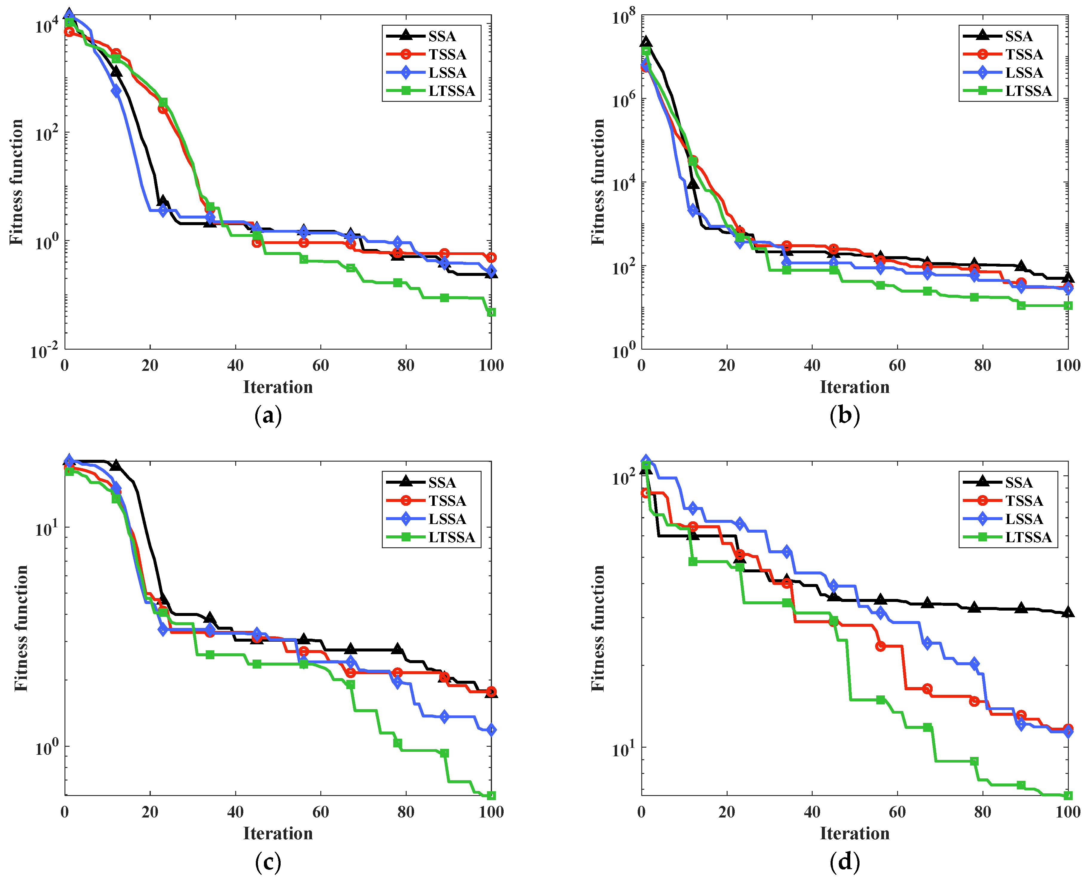
To further validate the impact of logistic–tent chaos on the initial population, representative test functions such as Sphere, Rosenbrock, Rastrigin, and Ackley were selected to evaluate the algorithm’s performance. These four functions were used to examine the algorithm’s convergence speed, convergence accuracy, global optimization capability, and global search ability. The population size was set to 100, and the maximum number of iterations was 100. The test results are shown in Figure 4.

As can be seen from Figure 4, the SSA algorithm incorporating logistic–tent chaotic mapping demonstrates significantly better convergence speed, convergence accuracy, global optimization capability, and global search ability compared to SSA with only tent mapping, logistic mapping, or without chaotic mapping. The introduction of logistic–tent chaos enhances the complexity and randomness of the chaotic system. Although it adds some computational complexity, performance evaluations have demonstrated its significant improvement in the algorithm’s performance, effectively increasing the quality of the initial population and strengthening the algorithm’s global search capability.

3.1.2. Refracted Opposition-Based Learning Schematic

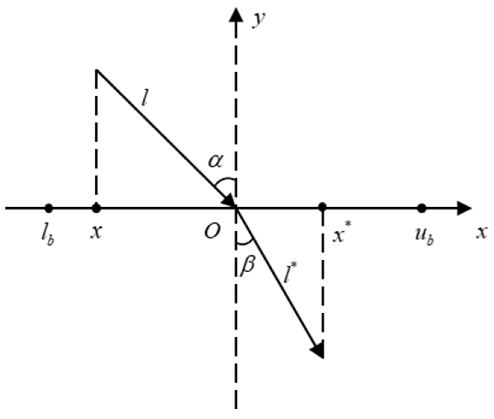
During the iterative updating of sparrow populations, it is easy to fall into local optima. To address this, a backward learning strategy based on the refraction principle is adopted to improve the initial population. This strategy introduces “pairwise points”, replacing random search with adversarial search, expanding the search range through inverse solutions of the current solution, and selecting individuals with higher fitness values for the next generation. Refractive backward learning, inspired by light refraction through transparent media, directs individuals closer to the optimal position more effectively than traditional strategies, reducing the likelihood of premature convergence.

Figure 5 shows the principle diagram of refractive inverse learning. The x-axis represents the search range of the solution $\left[l_b,u_b\right]$, while the y-axis represents the normal line.$l$ and $l^{*}$ denote the lengths of the incident and refracted rays, respectively. $\alpha$ and $\beta$ represent the angles of incidence and refraction, respectively.

From the definition of refractive index,

$$h={\displaystyle \frac{\sin \alpha }{\sin \beta }}={\displaystyle \frac{l^{*}((l_b+u_b)/2-x)}{l(x^{*}-(l_b+u_b)/2)}}$$

(7)

Let $m=l/l^{*}$ and by incorporating this into Equation (7), the refractive inverse solution is obtained as follows:

$$x^{*}={\displaystyle \frac{l_b+u_b}{2}}+{\displaystyle \frac{l_b+u_b}{2mh}}-{\displaystyle \frac{x}{mh}}$$

(8)

When h = m = 1, the refractive inverse solution can be transformed into the inverse learning formula $x^{*}=l_b+u_b-x$. This shows that refractive backward learning can reduce the probability of the algorithm falling into a local optimum by adjusting the solution space with parameters m and h. When the optimization problem extends to a higher-dimensional space, Equation (8) transforms into the following:

$$x_{i,j}^{*}={\displaystyle \frac{l_{bj}+u_{bj}}{2}}+{\displaystyle \frac{l_{bj}+u_{bj}}{2mh}}-{\displaystyle \frac{x_{i,j}}{mh}}$$

(9)

where $x_{i,j}$ is the j-th dimensional position of the i-th sparrow in the population; $x_{i,j}^{*}$ is the refracted reverse position of $x_{i,j}$; $l_{bj}$ and $u_{bj}$ are the minimum and maximum values in the j-th dimension of the search space, respectively.

3.1.3. Dynamic Adjustment of Population Size

In traditional SSA algorithms, the population size is usually fixed, which leads to noticeable differences in the algorithm’s performance when solving simple problems compared to complex ones. To address this issue, this paper proposes dynamically adjusting the population size using a linear approach. Specifically, in the initial stage of the search, a larger population size is set to better cover the search space, thereby enhancing the global search capability. As the number of iterations increases, the population size gradually decreases. This adjustment reduces computational cost while ensuring that different regions of the space are fully explored and individuals are gradually brought closer to the optimal solution. In the final stage of the algorithm, the population size is smaller, which helps the algorithm focus the search and perform fine local searches, further improving optimization accuracy. Throughout the dynamic adjustment process, the population size decreases gradually with the number of iterations to adapt to the search requirements at different stages, balancing exploration and exploitation capabilities. This improves the overall performance of the algorithm, especially when dealing with complex multi-peak optimization problems. The linear dynamic adjustment formula is as follows:

$$n_t=round[n_s-(n_s-n_f)\cdot (t/ite{r}_{\max })]$$

(10)

where $n_t$ denotes the population size for the current iteration number; $n_s$ denotes the initial population size; $n_f$ denotes the final population size.

3.2. Improvements in Location Updating

3.2.1. Incorporating the Golden Sine to Improve the Discoverer’s Position

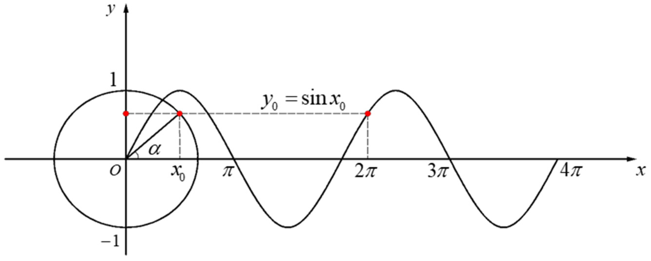
The Golden Sine Algorithm (Golden-SA) is a meta-heuristic algorithm proposed by Tanyildizi [32] in 2017. Inspired by the sine function and the golden section coefficient, the algorithm offers advantages such as rapid convergence, good robustness, and ease of implementation. Its core idea is to combine the sine function with the golden section coefficient to traverse the entire unit circle, thus achieving global search. In the Golden Sine Algorithm, there is a close mathematical relationship between the sine function and the unit circle, as illustrated in Figure 6. The coordinates on the sine function correspond to the y-axis coordinates of the points on the unit circle centered on the origin with a radius of 1. By traversing the points on the sine function, the algorithm enhances its global search capability. The introduction of the golden section coefficient in the position update process separates the solution space of each iteration, narrows the search area, explores the optimal solution region, enhances local exploration ability, and improves the convergence speed and accuracy of the algorithm.

The core process of the Golden Sine Algorithm is its position update formula. Initially, individuals are randomly generated, and the position update formula for each individual is as follows:

$$X_i^{t+1}=X_i^t\cdot \left|\sin (r_1)\right|-r_2\cdot \sin (r_1)\cdot \left|c_1{P}_p^t-c_2{X}_i^t\right|$$

(11)

where $P_i^t=(P_{i1},P_{i2},\cdots ,P_{id})$ denotes the optimal position of the individual in the t-th generation; $r_1$ is a random number in $[0,2\pi ]$, which determines the moving distance of the individual in the next iteration; $r_2$ is a random number in $[0,\pi ]$, which determines the moving direction of the individual in the next iteration; $c_1$ and $c_2$ are coefficients derived by introducing the golden ratio, an irrational number denoted by g, where $g=(\sqrt{5}-1)/2$, $c_1=-\pi +(1-g)\cdot 2\pi$, $c_2=-\pi +g\cdot 2\pi$. These coefficients serve to reduce the search space and guide the individual toward the global optimal position during the iteration process.

From the rules of the SSA, it is clear that discoverers have a high energy value and are responsible for leading the entire population in foraging. However, the lack of effective communication between discoverers within the population leads to a rapid approach to the global optimal solution at the beginning of the iteration, which can result in premature convergence. To address this deficiency, the golden sine mechanism is introduced to improve the discoverer position update method. The improved discoverer position update method is as follows:

$$X_{i,j}^{t+1}=\left\{\begin{array}{ll}{X}_{i,j}^t\cdot \left|\sin (r_1)\right|-r_2\cdot \sin (r_1)\cdot \left|c_1{X}_p^t-c_2{X}_{i,j}^t\right|\hfill & \hfill R_2<ST\\ X_{i,j}^t+Q·L\hfill & \hfill R_2\ge ST \end{array}\right.$$

(12)

In the improved position update formula, each sparrow exchanges information with the optimal individual, addressing the SSA’s deficiency in information exchange. The Golden Sine Algorithm expands the search space, enhancing global search capability and reducing the risk of local optima. The gradual reduction of the golden section coefficient optimizes the search process by adjusting the sparrow’s search distance and direction, balancing global exploration and local exploitation.

3.2.2. Spiral Search Mechanism Improves the Follower’s Position

According to the sparrow’s foraging principle, the discoverer is responsible for finding the food source, while the follower updates its position based on the discoverer’s position. This iterative updating near the optimal individual often causes most individuals to cluster around the optimal solution, leading to local optima and making the follower’s search direction unclear and its path unstable. Local optimization and global optimization are two key stages in optimization algorithms. Excessive local optimization limits the algorithm’s ability to explore the global optimal solution, while excessive global optimization may reduce search accuracy. To balance local and global search capabilities, a spiral search mechanism is introduced into the follower’s position update process. The improved follower position update formula is as follows:

$$X_{i,j}^{t+1}=\left\{\begin{array}{l}Q\cdot \exp \left({\displaystyle \frac{X_{worst}-X_{i,j}^t}{i^2}}\right) if i>n/2\\ X_p^{\mathrm{t}+1}+u\cdot \left|X_{i,j}^t-X_p^{\mathrm{t}+1}\right|\cdot A^{+}\cdot L \mathrm{otherwise}\end{array}\right.$$

(13)

$$u={\mathrm{e}}^{bv}\cdot \cos (2\pi b)$$

(14)

$$v=e^{k\cos (\pi (1-(t/ite{r}_{\max })))}$$

(15)

where b is a random number uniformly distributed on (0,1). The parameter k influences the search range of the algorithm. In this study, k is set to 5. The parameter v decreases with the increase in the number of iterations. The parameter u is a dynamic adjustment parameter, causing the follower’s position to spiral toward the optimal individual as iterations increase.

This improved strategy enables followers to conduct wide-ranging searches early on using the spiral curve, gradually reducing the search amplitude later. This enhances local optimization and convergence. The spiral search mechanism boosts followers’ autonomous search ability, decreasing the search range over time. This leads to the early discovery of high-quality solutions and reduces unnecessary searches later, enhancing global search capability, minimizing local optima traps, and balancing global and local search abilities, thereby improving overall performance.

3.3. Introduction of Differential Evolutionary Algorithms

In later iterations of the SSA algorithm, individuals tend to cluster near the optimal solution, affecting convergence accuracy. The Differential Evolution (DE) algorithm, introduced by Storn et al. [33], optimizes through mutation, crossover, and selection, offering good global search ability and robustness. Integrating DE into the SSA algorithm improves convergence accuracy and global optimization. The process for DE with a population size of n and dimension d is as follows:

Three individuals $x_{r_1}^t,x_{r_2}^t,x_{r_3}^t$ are randomly selected in the t-th iteration, and their mutation vectors are generated as follows:

$$v_i^t=x_{r_1}^t+F\cdot (x_{r_2}^t-x_{r_3}^t)$$

(16)

where F is the mutation operator used to control the probability of mutation, and $i=1,2,\cdots ,n$.

With a certain probability, the newly generated mutant individuals are allowed to cross-combine with the individuals in the original population to enhance the diversity of the population. The trial vector is generated as follows:

$$u_{i,j}^{t+1}=\left\{\begin{array}{l}{v}_{i,j}^{t+1} ,a_j\le CR or a_j= rnbr(i)\\ x_{i,j}^{t+1} ,\mathrm{otherwise}\end{array}\right.$$

(17)

where $a_j$ denotes the j-th $(j=1,2,\cdots ,d)$ computed random number obeying the uniform distribution [0,1]; $CR\in \left[0, 1\right]$ is the crossover operator; $rnbr(i)\in (1,2,\cdots ,d)$ is a randomly chosen index that ensures $u_{i,j}^{t+1}$ obtains at least one variable from $v_{i,j}^{t+1}$.

The trial vector $u_{i,j}^{t+1}$ is compared with the current target vector $x_{i,j}^t$ using the greedy algorithm to determine whether the trial vector evolves as follows:

$$x_i^{t+1}=\left\{\begin{array}{l}{u}_i^{t+1}, if f(u_i^{t+1})<f(x_i^t)\\ x_i^t , otherwise\end{array}\right.$$

(18)

3.4. Implementation Process of the Multi-Strategy Improved Sparrow Search Algorithm

The LDESSA algorithm enhances the initial population’s uniformity using logistic–tent chaotic mapping and improves quality with refractive reverse learning. It dynamically decreases the population size over time. The golden sine algorithm refines discoverer position updates, while the spiral search strategy improves follower updates. Finally, differential evolution boosts optimization capability. The pseudocode of the LDESSA algorithm is illustrated in Algorithm 1.

Algorithm 1: Pseudo-code of the LDESSA algorithm.

Input:         $ite{r}_{\max }$: the maximum iterations         PD: proportion of the discoverers         SD: proportion of the scouts         $R_2$: the warning value         $n_s$: initial population size         $n_f$: final population size Initialize a population:         a. Generate the initial population using logistic–tent chaotic mapping;         b. Apply refractive reverse learning to enhance diversity. Calculate the fitness of each search agent. Sort the population by fitness values to identify the current best and worst individuals. t = 1 while $t<ite{r}_{\max }$         Dynamic adjustment of population size by Equation (10)         $n_t$ = dynamic_population_size($n_s$, $n_f$, t, $ite{r}_{\max }$)         Sort the population by fitness values         for each individual i = 1 to $n_t$                 if i $\le n_t\cdot$PD                         Update discoverer location by Equation (12)                 else if > $n_t\cdot$PD                         Update follower location by Equation (13)                 end if                 if i $\le n_t\cdot$SD                         Update scout location by Equation (5)                 end if       end for       Perform differential evolution on the population by Equations (16)~(18)       Recalculate fitness values after updates       t = t + 1 end while return: $X_{best}$, $f_g$

4. Algorithm Performance Testing

To better validate the performance of the LDESSA algorithm, we selected 16 benchmark test functions for experimental evaluation. These include seven unimodal test functions, five high-dimensional multimodal test functions, and four low-dimensional multimodal test functions. LDESSA is compared and analyzed with the original sparrow search algorithm (SSA), the grey wolf optimizer (GWO), and particle swarm optimization (PSO), which are three high-performing path planning algorithms. The performance assessment is based on the convergence speed and convergence accuracy of the algorithms on the target test functions.

4.1. Benchmark Test Functions

Benchmark test functions are used to measure the convergence, stability, and other performance aspects of algorithms. They mainly include three types: unimodal test functions, high-dimensional multimodal test functions, and low-dimensional multimodal test functions. The benchmark test functions selected in this paper, along with their initialization spaces and optimal values, are shown in

Table 1. Benchmarking functions.

Function	Dim	Range	${\mathit{F}}_{\mathbf{min}}$
$F_1(x)={\displaystyle {\sum }_{i=1}^n{x_i}^2}$	30	[−100,100]	0
$F_2(x)={\displaystyle {\sum }_{i=1}^n\left|x_i\right|}+{\displaystyle {\coprod }_{i=1}^n\left|x_i\right|}$	30	[−10,10]	0
$F_3(x)={{\displaystyle {\sum }_{i=1}^n\left({\displaystyle {\sum }_{j=1}^i{x}_j}\right)}}^2$	30	[−100,100]	0
$F_4(x)={\max }_i\left\{\left|x_i\right|,1\le i\le n\right\}$	30	[−100,100]	0
$F_5(x)={\displaystyle {\sum }_{i=1}^{n-1}\left[100{(x_{i+1}-{x_i}^2)}^2+{\left(x_i-1\right)}^2\right]}$	30	[−30,30]	0
$F_6\left(x\right)={\displaystyle {\sum }_{i=1}^n{\left(\left[x_i+0.5\right]\right)}^2}$	30	[−100,100]	0
$F_7\left(x\right)={\displaystyle {\sum }_{i=1}^{n}i{x_i}^4+random\left[0,1\right)}$	30	[−1.28,1.28]	0
$F_8\left(x\right)={\displaystyle {\sum }_{i=1}^n-x_i\sin x\left(\sqrt{\left|x_i\right|}\right)}$	30	[−500,500]	−418.829n
$F_9(x)={\displaystyle {\sum }_{i=1}^n\left[{x_i}^2-10\cos \left(2\pi x_i\right)+10\right]}$	30	[−5.12,5.12]	0
$F_{10}(x)=-20\exp (-0.2\sqrt{\left(1/n\right){\displaystyle {\sum }_{i=1}^n{x_i}^2}})-\exp \left[(1/n){\displaystyle {\sum }_{i=1}^n\cos (2\pi x_i)}\right]+20+e$	30	[−32,32]	0
$F_{11}\left(x\right)=\left(1/4000\right){\displaystyle {\sum }_{i=1}^n{x_i}^2}-{\displaystyle {\prod }_{i=1}^n\cos \left(x_i/\sqrt{i}\right)}+1$	30	[−600,600]	0
$F_{12}(x)=(\pi /n)\left\{10\sin (\pi y_1)+{\displaystyle {\sum }_{i=1}^{n-1}{(y_i-1)}^2[1+10{\sin }^2(\pi y_{i+1})]+{(y_n-1)}^2}\right\}+$${\displaystyle {\sum }_{i=1}^{n}u(x_i,10,100,4)},y_i=1+{\displaystyle \frac{x_i+1}{4}},u(x_i,a,k,m)=\left\{\begin{array}{l}k{(x_i-a)}^m x_i>a\\ 0 -a<x_i<a\\ k{(-x_i-a)}^m x_i>a\end{array}\right.$	30	[−50,50]	0
$F_{13}(x)={\displaystyle {\sum }_{i=1}^4{c}_i\exp (-{\displaystyle {\sum }_{j=1}^6{a}_{ij}{(x_j-p_{ij})}^2}}$	6	[0,1]	−3.32
$F_{14}(x)=((1/500)+{\displaystyle {\sum }_{j=1}^{25}1/(j+{\displaystyle {\sum }_{i=1}^2{(x_i-a_{ij})}^6){)}^{-1}}}$	2	[−65.536,65.536]	0.998
$F_{15}(x)={\displaystyle {\sum }_{i=1}^{11}{(a_i-(x_1({b_i}^2+b_1{x}_2)/({b_i}^2+b_1{x}_3+x_4)))}^2}$	4	[−5,5]	0.0003
$F_{16}(x)=4{x_1}^2-2.1{x_1}^4+(1/3){x_1}^6+x_1{x}_2-4{x_2}^2+4{x_2}^4$	2	[−5,5]	−1.032

. Among them, $F_1\sim F_7$ are unimodal test functions, which have only one extremum point and are used to verify the convergence speed, convergence accuracy, and robustness of the algorithm in simple environments. $F_8\sim F_{12}$ are high-dimensional multimodal test functions, which have multiple extremum points and are used to evaluate the algorithm’s ability to find the global optimal solution in complex environments. $F_{13}\sim F_{16}$ are low-dimensional multimodal test functions, further testing the algorithm’s stability and optimization capability.

4.2. Tests and Analysis of Results

The algorithm performance testing experiments in this paper were conducted using MATLAB 2020b on a Windows 11 system with a 2.50 GHz Intel i9 processor and 32 GB of RAM. To enhance the global search capability of the algorithm, the proportion of discoverers (PD) in the LDESSA algorithm was set to 0.6. Multiple experiments have shown that the improved LDESSA algorithm effectively balances global search and local exploitation at PD = 0.6. It was found experimentally that the performance of the SSA algorithm was significantly lower when the discoverer ratio was set to PD = 0.6 compared to PD = 0.2, with the SSA algorithm performing best at PD = 0.2. Therefore, this paper compares the LDESSA algorithm with the best-performing SSA algorithm (PD = 0.2). The population size of the PSO, GWO, and SSA algorithms was set to n = 100, while the LDESSA algorithm dynamically adjusted the population size to $n_s=100$ and $n_f=20$. The maximum number of iterations for all algorithms was set to $ite{r}_{\max }=1000$. Other parameter settings are shown in

Table 2. Algorithm parameter settings.

Algorithm	Params
PSO	$c_1=c_2=2,w=0.9$
GWO	$a\in [0,2]$, decreases linearly from 2 to 0
SSA	$PD=0.2,SD=0.2,ST=0.8$
LDESSA	$PD=0.6,SD=0.2,ST=0.8$

. To ensure the stability and reliability of the experimental results, each experiment was run independently 30 times. The optimal value, mean value, and standard deviation of the objective function were recorded and compared. The specific experimental results are shown in

Table 3. Optimization results for each algorithm.

Function	Algorithm	Best	Ave	Std
$F_1(x)$	PSO	4.7911 × 10−6	1.7928 × 10−5	1.1009 × 10−5
	GWO	3.6428 × 10−183	1.6639 × 10−178	0
	SSA	0	0	0
	LDESSA	0	0	0
$F_2(x)$	PSO	7.1096 × 10−2	1.3159 × 10−2	4.8649 × 10−3
	GWO	1.6562 × 10−101	1.6749 × 10−98	4.9533 × 10−98
	SSA	0	0	0
	LDESSA	0	0	0
$F_3(x)$	PSO	1.6755 × 10−4	4.9754 × 10−4	2.8125 × 10−5
	GWO	2.2164 × 10−92	7.4565 × 10−86	2.1289 × 10−85
	SSA	0	0	0
	LDESSA	0	0	0
$F_4(x)$	PSO	1.8722 × 10−3	5.6178 × 10−3	2.9665 × 10−3
	GWO	3.6481 × 10−61	2.9002 × 10−58	8.7856 × 10−58
	SSA	0	2.5597 × 10−306	2.7355 × 10−7
	LDESSA	0	0	0
$F_5(x)$	PSO	7.5667 × 10−1	5.4178	2.7355
	GWO	4.9011	5.7745	0.7487
	SSA	8.1068 × 10−13	1.5956 × 10−9	1.9279 × 10−8
	LDESSA	4.5841 × 10−24	8.4803 × 10−17	1.3131 × 10−16
$F_6(x)$	PSO	1.3295 × 10−5	1.8931 × 10−5	1.2207 × 10−5
	GWO	1.2551 × 10−7	4.5469 × 10−7	1.3865 × 10−7
	SSA	0	0	0
	LDESSA	1.1093 × 10−31	3.8661 × 10−29	4.6147 × 10−29
$F_7(x)$	PSO	1.5592 × 10−3	3.5651 × 10−3	2.0006 × 10−3
	GWO	1.3647 × 10−5	9.3145 × 10−5	6.7438 × 10−5
	SSA	1.6026 × 10−6	7.9944 × 10−5	5.5367 × 10−5
	LDESSA	1.0776 × 10−6	6.8833 × 10−5	4.9066 × 10−5
$F_8(x)$	PSO	−2.9264 × 103	−2.3837 × 103	3.4624 × 102
	GWO	−3.398 6 × 103	−2.9036 × 103	3.6221 × 102
	SSA	−3.8543 × 103	−3.4560 × 103	2.7040 × 102
	LDESSA	−3.8776 × 103	−3.4501 × 103	2.3350 × 102
$F_9(x)$	PSO	2.991	4.8978	1.5145
	GWO	0	0	0
	SSA	0	0	0
	LDESSA	0	0	0
$F_{10}(x)$	PSO	3.0512 × 10−3	4.4579 × 10−3	2.2087 × 10−3
	GWO	4.4409 × 10−15	4.4409 × 10−15	0
	SSA	8.8818 × 10−16	8.8818 × 10−16	0
	LDESSA	8.8818 × 10−16	8.8818 × 10−16	0
$F_{11}(x)$	PSO	1.6547 × 10−1	2.6188 × 10−1	9.2614 × 10−2
	GWO	0	2.7906 × 10−2	2.9144 × 10−2
	SSA	0	0	0
	LDESSA	0	0	0
$F_{12}(x)$	PSO	1.7353 × 10−6	4.7691 × 10−6	4.3299 × 10−6
	GWO	29859 × 10−8	9.0793 × 10−8	4.4215 × 10−8
	SSA	1.7118 × 10−32	4.7016 × 10−32	3.5118 × 10−32
	LDESSA	2.692 × 10−32	5.6966 × 10−31	2.7245 × 10−32
$F_{13}(x)$	PSO	−3.322	−3.2671	7.3707 × 10−2
	GWO	−3.322	−3.2606	8.2064 × 10−2
	SSA	−3.322	−3.2863	5.7434 × 10−2
	LDESSA	−3.322	−3.2982	5.0132 × 10−2
$F_{14}(x)$	PSO	9.98 × 10−1	9.98 × 10−1	0
	GWO	9.98 × 10−1	4.3244	4.5129
	SSA	9.98 × 10−1	2.3637	3.6747
	LDESSA	9.98 × 10−1	9.98 × 10−1	0
$F_{15}(x)$	PSO	3.0882 × 10−4	3.5486 × 10−4	6.2412 × 10−5
	GWO	3.0749 × 10−4	2.4046 × 10−4	0
	SSA	3.0749 × 10−4	3.0749 × 10−4	0
	LDESSA	3.0749 × 10−4	3.0749 × 10−4	0
$F_{16}(x)$	PSO	−1.0316	−1.0316	0
	GWO	−1.0316	−1.0316	0
	SSA	−1.0316	−1.0316	0
	LDESSA	−1.0316	−1.0316	0

.

4.2.1. Analysis of Single-Peak Test Functions

Based on the experimental results for unimodal test functions (as shown in Table 3), it is evident that the LDESSA algorithm successfully finds the optimal solution for functions $F_1\sim F_4$. Although it does not reach the optimal solution for functions $F_5$ and $F_7$, LDESSA’s mean and standard deviation are closer to the theoretical optimum compared to PSO, GWO, and SSA. However, in the case of function $F_6$, LDESSA’s convergence accuracy is slightly inferior to SSA. 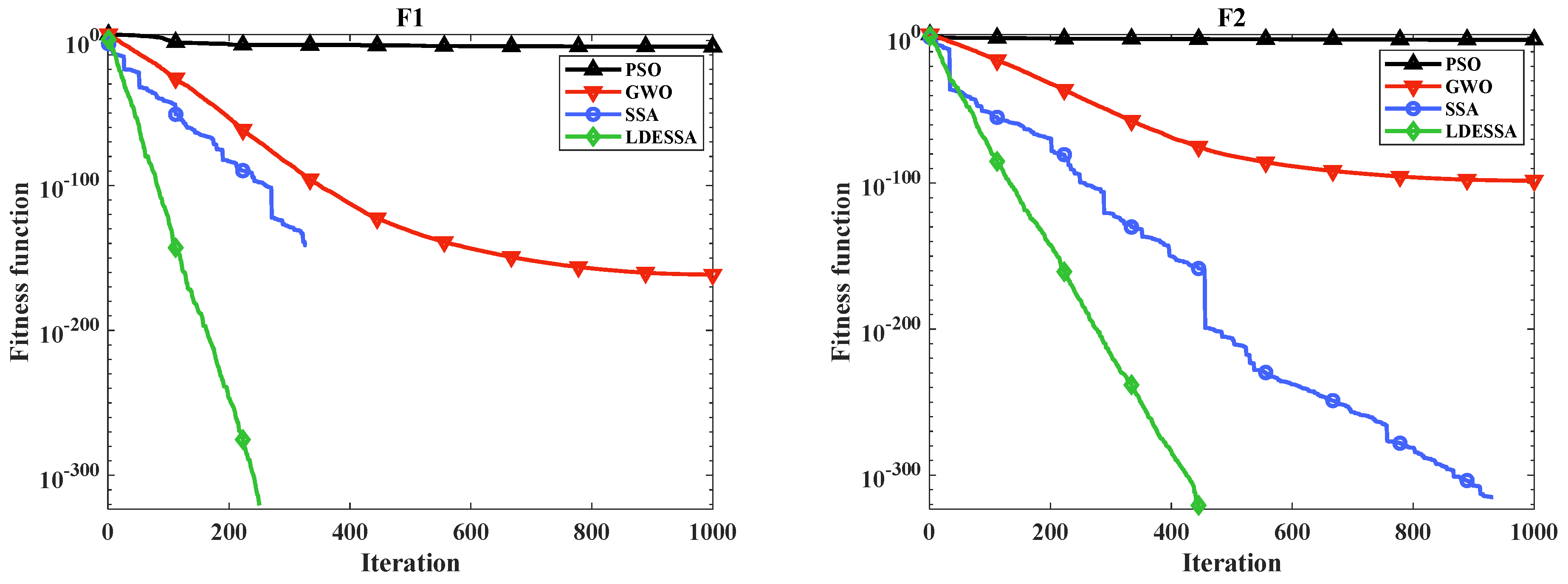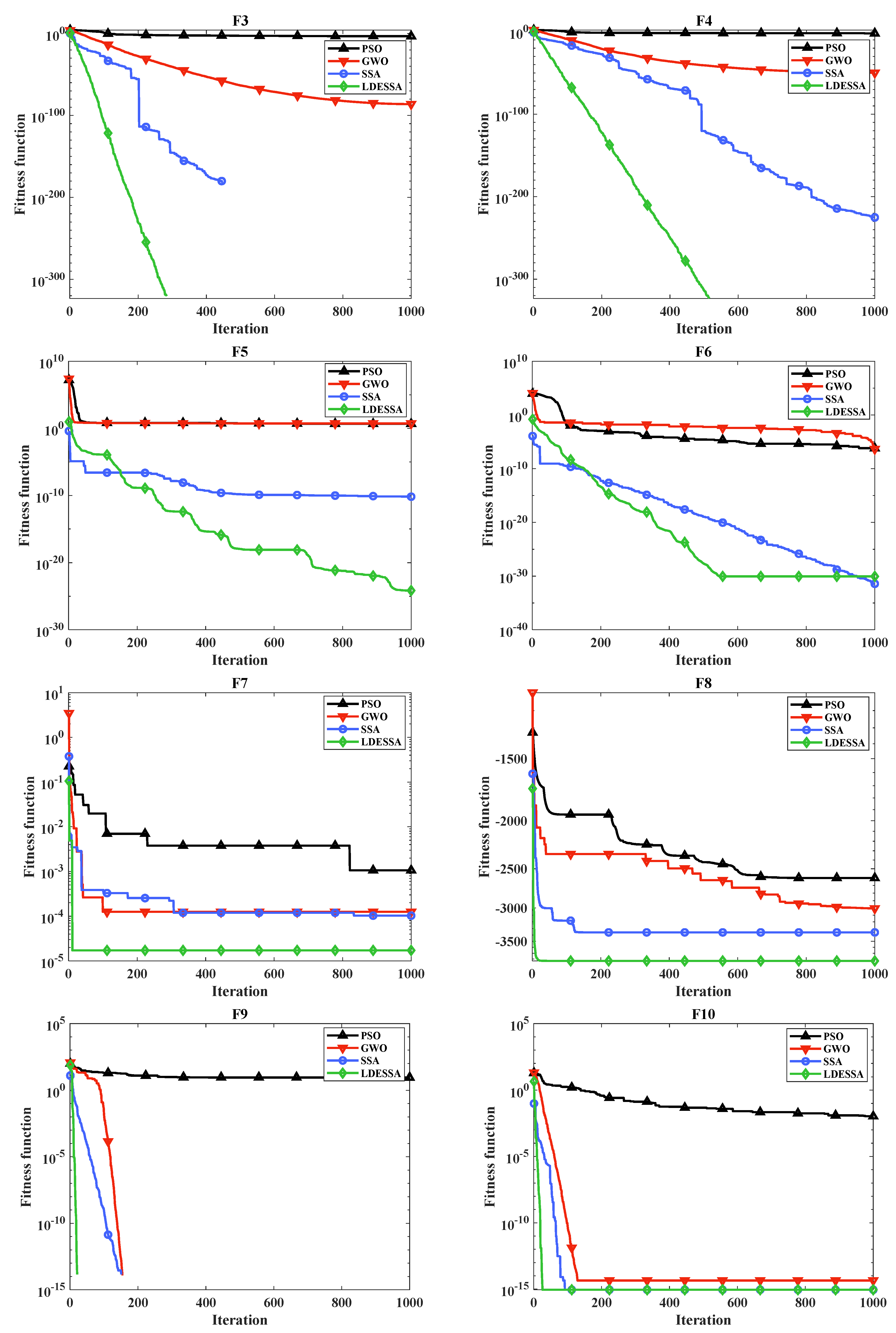This is because $F_6$ is a simple quadratic function, and LDESSA introduces strategies to increase the initial population’s diversity. While this diversity is advantageous for complex functions by promoting thorough exploration of the search space, it may lead to individuals being more dispersed during the initial search phase for this objective function. This dispersion could potentially impact the final convergence accuracy. From the convergence curves of the algorithms on the single-peak test functions (Figure 7), it is evident that the LDESSA algorithm converges significantly better than the other three algorithms on functions $F_1\sim F_5$, especially on functions $F_1$ and $F_3$, achieving high-precision convergence in about 300 generations. In summary, the LDESSA algorithm demonstrates strong stability and excellent optimization capability in simple environments.

4.2.2. Analysis of High-Dimensional Multimodal Test Functions

Analyzing the results for high-dimensional multimodal test functions (as shown in Table 3), the LDESSA algorithm outperforms the other three algorithms in terms of mean values for functions $F_9\sim F_{11}$, demonstrating higher convergence accuracy. For function $F_8$, LDESSA achieves a more optimal value due to the introduction of the spiral search mechanism in the follower position update, which enhances local search in complex spaces. However, LDESSA’s mean value is slightly higher than that of SSA. This outcome might be attributed to the dynamic population adjustment strategy in LDESSA, where the population size decreases as iterations progress. While this aids in focused searching in later stages, it may also limit the exploration of the search space, leading to a slightly higher average value. For the complex function $F_{12}$, neither LDESSA nor SSA was able to converge to the optimal solution. LDESSA’s optimal and mean values were slightly higher, likely due to the spiral search mechanism, which enhanced local search capability, aiding in fine-tuning the search in this complex space but potentially causing the algorithm to focus prematurely during the early or middle stages, thus limiting broader exploration. However, the combination of the spiral search mechanism and differential evolution allowed LDESSA to effectively avoid premature convergence on a broader scale in complex multimodal environments, demonstrating robust global search capability and stability. As shown in Figure 7, LDESSA consistently exhibited a significantly faster convergence rate compared to the other three algorithms. In summary, while LDESSA has some limitations in complex, high-dimensional multimodal environments, it still outperforms SSA overall. LDESSA demonstrates superior stability and strong global search capability, effectively balancing global and local search.

4.2.3. Analysis of Low-Dimensional Multimodal Test Functions

For low-dimensional multimodal test functions, Table 3 shows that the LDESSA algorithm’s average values for functions $F_{13}\sim F_{15}$ are closest to the optimal among the four algorithms. Additionally, the standard deviation for functions $F_{14}\sim F_{16}$ is zero, and for function $F_{13}$, it is the smallest among the four algorithms, indicating excellent stability. As illustrated in Figure 7, the LDESSA algorithm also has the fastest convergence speed among the four algorithms. In summary, the experimental results in low-dimensional multimodal environments further confirm that the LDESSA algorithm performs exceptionally well in less complex environments, demonstrating excellent stability and rapid convergence capabilities.

4.2.4. Overall Performance

Overall, the LDESSA algorithm significantly improves the performance of the traditional SSA algorithm across various test functions. It excels in unimodal, high-dimensional multimodal, and low-dimensional multimodal test environments, demonstrating not only rapid convergence but also the ability to find near-optimal solutions. This showcases its strong global search capability and stable optimization performance. By incorporating multiple strategy improvement mechanisms, the LDESSA algorithm effectively avoids local optima traps during the optimization process, enhancing both the convergence speed and solution quality.

5. Path Planning Simulation Analysis

To verify the effectiveness of the LDESSA algorithm in bridge inspection applications, path planning simulation experiments were conducted under the environmental conditions described in Section 4.2. Under identical experimental conditions, the performance of the LDESSA algorithm was compared and analyzed alongside other high-performing path planning algorithms: PSO, GWO, and SSA.

5.1. Environmental Modeling

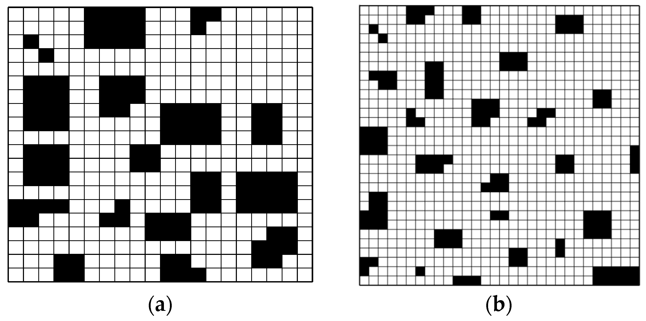
The surface of the bridge structure can be regarded as a two-dimensional plane, with the environment map model constructed using the raster map method. In this model, areas inaccessible to wall-climbing robots, such as obvious cracks and hollow drums, are considered obstacles. These obstacles are represented as black rasters on the map, while free areas are represented as white rasters, corresponding to 1 and 0 in the matrix, respectively. The working environment of wall-climbing robots was simulated using MATLAB, constructing two types of raster environment maps with varying levels of complexity, as shown in Figure 8. The specifications for Environment 1 and Environment 2 are 20 × 20 and 30 × 30, respectively.

5.2. Energy Consumption Modeling

In the bridge inspection process, the wall-climbing robot is unable to carry a large-capacity battery due to weight limitations, resulting in high requirements for energy consumption. The robot’s energy consumption is closely related to the path planning length, the number of turns, and the steering angle. To verify the performance of the LDESSA algorithm in bridge inspection path planning, energy consumption is used as the evaluation criterion to analyze the path planning effectiveness of each algorithm. The relationship between the indicators is as follows:

$$\left\{\begin{array}{l}E=E_s+E_{\theta }\\ E_s=L\cdot e\\ E_{\theta }={\displaystyle {\sum }_{i=1}^p{E}_{\theta ,i}}\\ E_{\theta ,i}=k{\theta }_i+\delta \end{array}\right.$$

(19)

where E is the total energy consumption of the robot; $E_s$ and $E_{\theta }$ represent the energy consumed by the robot walking and steering, respectively; L is the path planning length; the parameter e is the energy consumed per unit length of path planning, set at 15 J/unit length in this study; the parameter p is the number of turns; the parameter ${\theta }_i$ is the steering angle of the i-th turn, with ${\theta }_i\in [{20}^{\circ },{180}^{\circ }]$. The energy consumed by steering varies with the steering angle, with larger angles resulting in higher energy consumption, and steering energy consumption is not considered when the angle is less than 20°. The steering energy consumption coefficient k is set at 0.5°/J. The parameter ẟ is a constant, set at 30 J in this study.

5.3. Simulation Experiment and Result Analysis

To verify the performance of the LDESSA algorithm in bridge inspection path planning, simulation experiments were conducted for the PSO, GWO, SSA, and LDESSA algorithms. The population sizes for the PSO, GWO, and SSA algorithms were set to 50, while the population size for the LDESSA algorithm was set dynamically to $n_s=50$ and $n_f=20$. 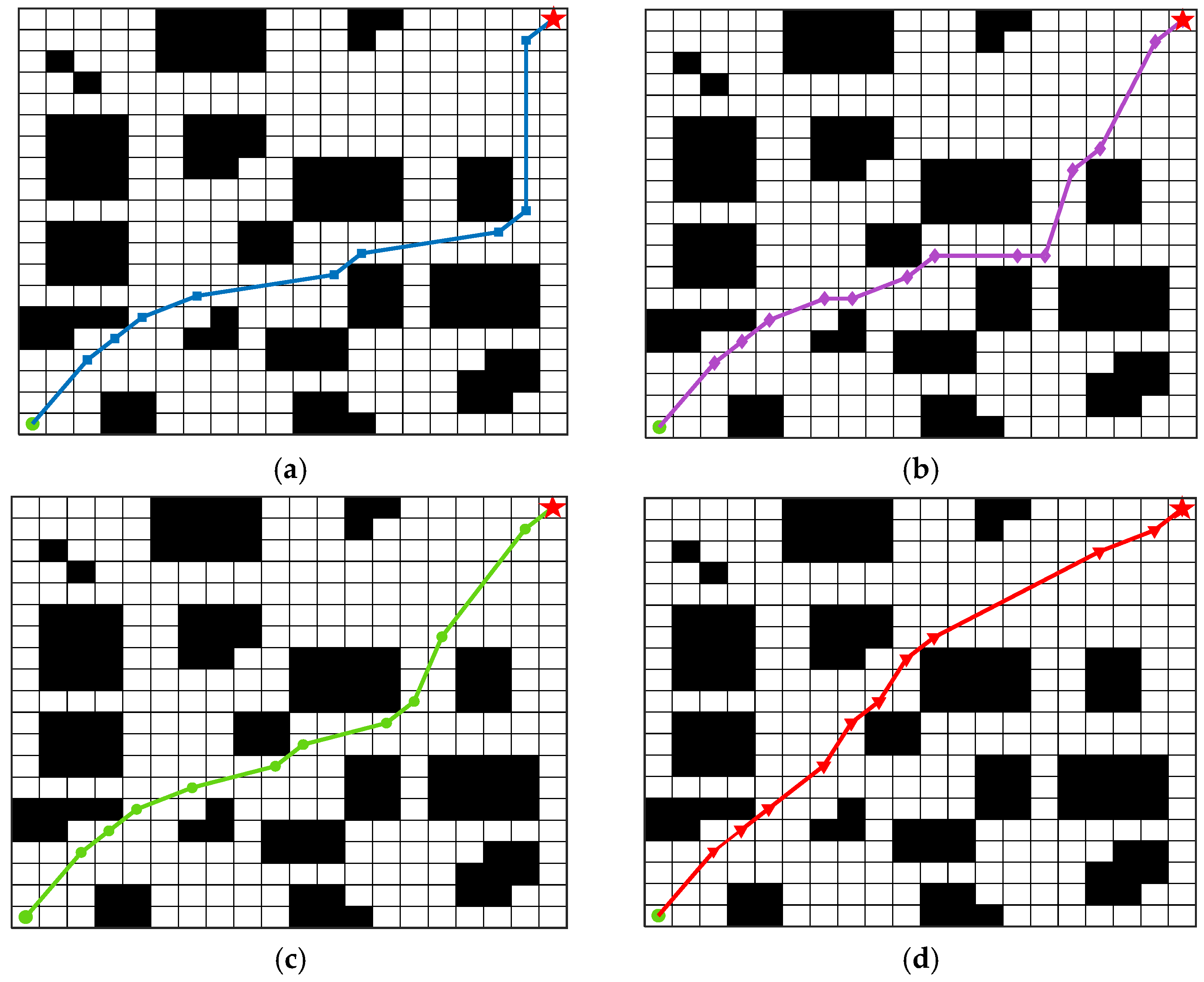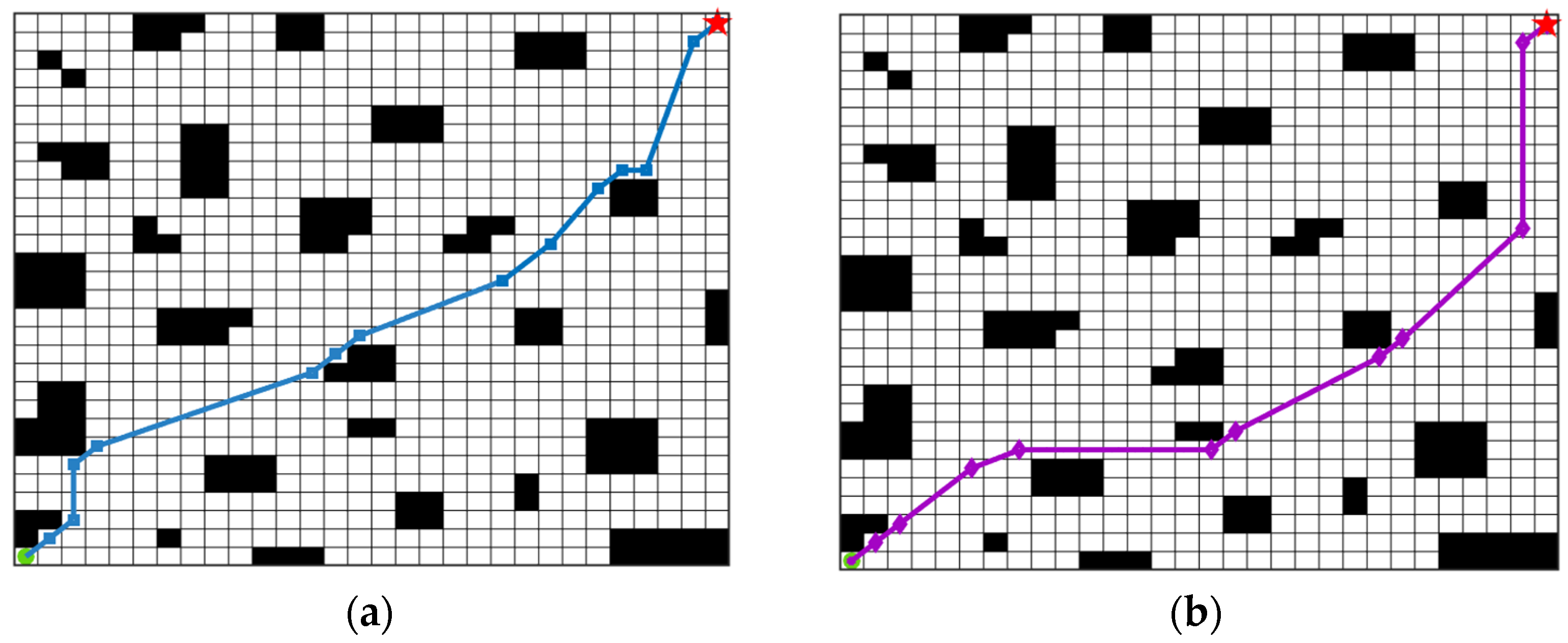The maximum number of iterations was set to $ite{r}_{\max }=200$, with other parameters as shown in Table 2. To ensure the accuracy of the simulation experiments, each algorithm was run 10 times individually. The average values of energy consumption, path length, number of turns, and maximum steering angle were recorded and compared to determine the optimal energy consumption path planning results, as shown in Figure 9 and Figure 10. The results of the simulation experiments for each algorithm are presented in

Table 4. Comparison of performance indicators for algorithms (PSO, GWO, SSA, LDESSA).

Map	Algorithm	Path Len	Turns	Max Angle (°)	Energy (J)
Environment 1	PSO	31.1	5	65.96	762.22
	GWO	29.66	6	53.2	729.84
	SSA	28.23	4	32.16	596.59
	LDESSA	27.42	2	29.57	537.05
Environment 2	PSO	49.27	6	68.46	1145.34
	GWO	46.65	5	51.71	1044.53
	SSA	43.62	4	46.61	904.14
	LDESSA	42.83	2	36.74	799.86

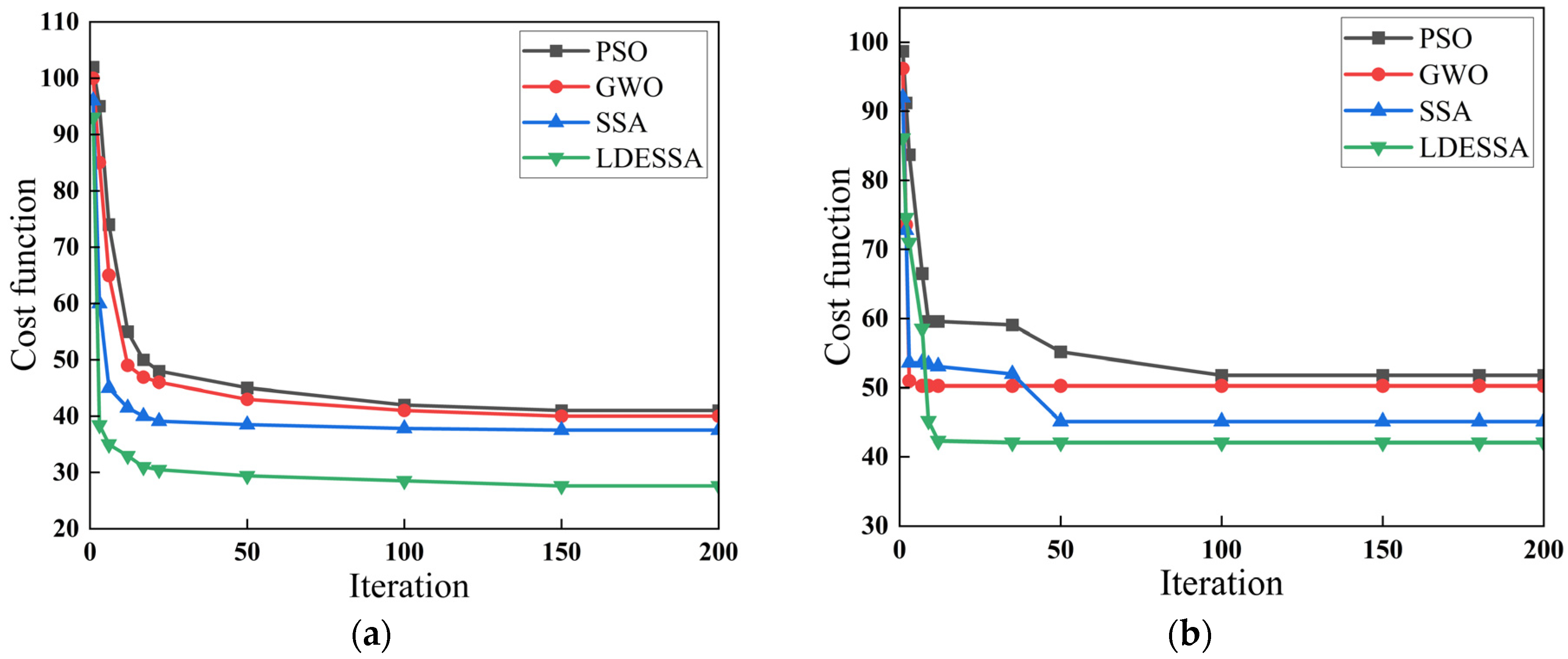
, with the convergence curves of the cost function shown in Figure 11.

Analysis of the above experimental results indicates that the LDESSA algorithm performs best in terms of energy consumption for path planning in both environments. Compared to SSA, the LDESSA algorithm reduces energy consumption by 9.98% in Environment 1 and 11.50% in Environment 2. It also significantly outperforms the other three algorithms in terms of path length, number of turns, and maximum steering angle. Especially in the more complex Environment 2, the advantage of the LDESSA algorithm is more pronounced, demonstrating its superior ability to find the optimal path in complex environments. The convergence curves of the cost function (Figure 11) show that the proposed method has faster convergence speed and higher convergence accuracy, proving its high applicability in bridge inspection path planning.

6. Conclusions

This paper presents an improved sparrow search algorithm (LDESSA) based on logistic–tent mapping and differential evolution, which effectively enhances the global optimization capability of SSA by integrating multiple strategies, addressing its tendency to get trapped in local optima. Firstly, logistic–tent chaotic mapping is used to create a more homogeneous initial population, which is then diversified through refractive reverse learning, while the dynamically adjusted population size during iterations balances global search and local exploitation abilities. Secondly, the position update method for discoverers is improved by incorporating the golden sine algorithm, enhancing local exploration. Additionally, a spiral search mechanism is used to update follower positions, helping the algorithm escape local optima. Finally, differential evolution is introduced to further enhance the algorithm’s global search capability. The optimization ability of the LDESSA has been validated by 16 benchmark functions. A simulation experiment of bridge inspection path planning for wall-climbing robots further validates the algorithm’s effectiveness, demonstrating clear advantages in environments with varying complexity. Compared to SSA, the LDESSA algorithm reduces energy consumption by 9.98% in Environment 1 and 11.50% in Environment 2. Additionally, it outperforms other algorithms in terms of path length, number of turns, and maximum steering angle.

Although the LDESSA algorithm has made significant progress in terms of global optimization and effectiveness, the integration of multiple enhancement strategies has resulted in increased response times in complex environments. To address this issue, future research should focus on improving the algorithm’s operational efficiency without compromising its optimization capabilities. In addition, further research is necessary to explore the algorithm’s practical application in bridge inspection. This research would focus on addressing potential challenges in real-world scenarios, such as managing complex dynamic environments and overcoming computational resource limitations.

References

- Fu, Y.; Li, H. Researching headway of wall-climbing robots. J. Mach. Des. 2008, 4, 1–5. [Google Scholar] [CrossRef]
- Wu, S.; Li, M.; Xiao, S.; Li, Y. A wireless distributed wall climbing robotic system for reconnaissance purpose. In Proceedings of the 2006 IEEE International Conference on Mechatronics and Automation, Luoyang, China, 25–28 June 2006. [Google Scholar] [CrossRef]
- Qian, Z.-Y.; Zhao, Y.-Z.; Fu, Z.; Cao, Q.-X. Design and realization of a non-actuated glass-curtain wall-cleaning robot prototype with dual suction cups. Int. J. Adv. Manuf. Technol. 2006, 30, 147–155. [Google Scholar] [CrossRef]
- Han, L.; Wang, L.; Zhou, J.; Wang, Y. The development status of ship wall-climbing robot. In Proceedings of the 2021 4th International Conference on Electron Device and Mechanical Engineering (ICEDME), Guangzhou, China, 19–21 March 2021. [Google Scholar] [CrossRef]
- Huang, H.; Li, D.; Xue, Z.; Chen, X.; Liu, S.; Leng, J.; Wei, Y. Design and performance analysis of a tracked wall-climbing robot for ship inspection in shipbuilding. Ocean. Eng. 2017, 131, 224–230. [Google Scholar] [CrossRef]
- Zhang, X.; Zhang, X.; Zhang, M.; Sun, L.; Li, M. Optimization design and flexible detection method of wall-climbing robot system with multiple sensors integration for magnetic particle testing. Sensors 2020, 20, 4582. [Google Scholar] [CrossRef] [PubMed]
- Zhang, H.-Y.; Lin, W.-M.; Chen, A.-X. Path planning for the mobile robot: A review. Symmetry 2018, 10, 450. [Google Scholar] [CrossRef]
- Dijkstra, E.W. A note on two problems in connexion with graphs. In Edsger Wybe Dijkstra: His Life, Work, and Legacy; Association for Computing Machinery: New York, NY, USA, 2022; pp. 287–290. [Google Scholar] [CrossRef]
- Hartomo, K.; Ismanto, B.; Nugraha, A.; Yulianto, S.; Laksono, B. Searching the shortest route to distribute disaster’s logistical assistance using Dijkstra method. J. Phys. Conf. Ser. 2019, 1402, 077014. [Google Scholar] [CrossRef]
- Bengio, Y. Deep learning of representations: Looking forward. In International Conference on Statistical Language and Speech Processing; Springer: Berlin/Heidelberg, Germany, 2013. [Google Scholar] [CrossRef]
- Hart, P.E.; Nilsson, N.J.; Raphael, B. A formal basis for the heuristic determination of minimum cost paths. IEEE Trans. Syst. Sci. Cybern. 1968, 4, 100–107. [Google Scholar] [CrossRef]
- Wang, F.; Gao, Y.; Chen, Z.; Gong, X.; Zhu, D.; Cong, W. A path planning algorithm of inspection robots for solar power plants based on improved RRT. Electronics 2023, 12, 4455. [Google Scholar] [CrossRef]
- Huang, Y.; Ding, H.; Zhang, Y.; Wang, H.; Cao, D.; Xu, N.; Hu, C. A motion planning and tracking framework for autonomous vehicles based on artificial potential field elaborated resistance network approach. IEEE Trans. Ind. Electron. 2019, 67, 1376–1386. [Google Scholar] [CrossRef]
- Holland, J.H. Genetic algorithms. Sci. Am. 1992, 267, 66–73. Available online: https://www.jstor.org/stable/24939139 (accessed on 12 October 2022). [CrossRef]
- Alam, T.; Qamar, S.; Dixit, A.; Benaida, M. Genetic algorithm: Reviews, implementations, and applications. arXiv 2020, arXiv:2007.12673. [Google Scholar] [CrossRef]
- Liu, X.; Tian, S.; Tao, F.; Yu, W. A review of artificial neural networks in the constitutive modeling of composite materials. Compos. Part B Eng. 2021, 224, 109152. [Google Scholar] [CrossRef]
- Turing, A.M. On computable numbers, with an application to the Entscheidungsproblem. J. Math. 1936, 58, 5. [Google Scholar] [CrossRef]
- Nayar, N.; Gautam, S.; Singh, P.; Mehta, G. Ant colony optimization: A review of literature and application in feature selection. Inven. Comput. Inf. Technol. Proc. ICICIT 2020, 2021, 285–297. [Google Scholar] [CrossRef]
- Kennedy, J.; Eberhart, R. Particle swarm optimization. In Proceedings of the ICNN’95-International Conference on Neural Networks, Perth, Australia, 27 November–1 December 1995. [Google Scholar] [CrossRef]
- Ghannadi, P.; Kourehli, S.S.; Mirjalili, S. A review of the application of the simulated annealing algorithm in structural health monitoring (1995–2021). Frat. Ed Integrità Strutt. 2023, 17, 51–76. [Google Scholar] [CrossRef]
- Kirkpatrick, S.; Jr, C.D.G.; Vecchi, M.P. Optimization by simulated annealing. Science 1983, 220, 671–680. [Google Scholar] [CrossRef]
- Xue, J.; Shen, B. A novel swarm intelligence optimization approach: Sparrow search algorithm. Syst. Sci. Control. Eng. 2020, 8, 22–34. [Google Scholar] [CrossRef]
- Li, J. Robot path planning based on improved sparrow algorithm. J. Phys. Conf. Ser. 2021, 1861, 012017. [Google Scholar] [CrossRef]
- Liu, G.; Shu, C.; Liang, Z.; Peng, B.; Cheng, L. A modified sparrow search algorithm with application in 3d route planning for UAV. Sensors 2021, 21, 1224. [Google Scholar] [CrossRef]
- Zhang, Z.; He, R.; Yang, K. A bioinspired path planning approach for mobile robots based on improved sparrow search algorithm. Adv. Manuf. 2022, 10, 17. [Google Scholar] [CrossRef]
- Gao, Q.; Zheng, J.; Zhang, W. Research on optimization of manned robot swarm scheduling based on ant-sparrow algorithm. J. Phys. Conf. Ser. 2021, 2078, 012002. [Google Scholar] [CrossRef]
- Sun, Z.; Zhang, B.; Cheng, L.; Zhang, W. Application of the redundant servomotor approach to design of path generator with dynamic performance improvement. Mech. Mach. Theory 2011, 46, 1784–1795. [Google Scholar] [CrossRef]
- Wang, J.; Wang, H.F.; Ip, W.H.; Furuta, K.; Kanno, T.; Zhang, W.J. Predatory search strategy based on swarm intelligence for continuous optimization problems. Math. Probl. Eng. 2013, 2013, 749256. [Google Scholar] [CrossRef]
- Shan, L.; Qiang, H.; Li, J.; Wang, Z.Q. Chaotic optimization algorithm based on Tent map. Control. Decis. 2005, 20, 179–182. [Google Scholar] [CrossRef]
- Zhang, H.; Zhang, T.N.; Shen, J.H.; Li, Y. TentResearch on decision-makings of structure optimization based on improved Tent PSO. Control. Decis. 2008, 23, 857–862. [Google Scholar] [CrossRef]
- Chen, Z.; Liang, D.; Deng, X. Performance Analysis and Improvement of Logistic Chaotic Mapping. J. Electron. Inf. Technol. 2016, 38, 1547–1551. [Google Scholar] [CrossRef]
- Tanyildizi, E.; Demir, G. Golden sine algorithm: A novel math-inspired algorithm. Adv. Electr. Comput. Eng. 2017, 17, 71. [Google Scholar] [CrossRef]
- Storn, R.; Price, K. Differential evolution–a simple and efficient heuristic for global optimization over continuous spaces. J. Glob. Optim. 1997, 11, 341–359. [Google Scholar] [CrossRef]
Figure 1.
Histogram of chaotic mapping: (a) tent mapping; (b) logistic mapping; (c) logistic–tent mapping.
Figure 2.
Scatter plot of chaotic mapping: (a) tent mapping; (b) logistic mapping; (c) logistic–tent mapping.
Figure 3.
Lyapunov exponent analysis of logistic–tent mapping.
Figure 4.
Convergence curves of standard and chaos-based SSA variants: (a) Sphere; (b) Rosenbrock; (c) Rastrigin; (d) Ackley. Figure labels: TSSA (SSA with tent map), LSSA (SSA with logistic map), LTSSA (SSA with logistic–tent map).
Figure 5.
Refractive inverse learning schematic.
Figure 6.
Relationship between the unit circle and the sinusoidal function curve.
Figure 7.
Convergence curves on the test functions of each algorithm.
Figure 8.
Map of the two complexity levels of the environment: (a) Environment 1; (b) Environment 2.
Figure 9.
Simulation of path planning for each algorithm in Environment 1: (a) PSO; (b) GWO; (c) SSA; (d) LDESSA. The starting point is shown as a green dot, and the end point is shown as a red dot.
Figure 10.
Simulation of path planning for each algorithm in Environment 2: (a) PSO; (b) GWO; (c) SSA; (d) LDESSA. The starting point is shown as a green dot, and the end point is shown as a red dot.
Figure 11.
Cost function convergence curve: (a) Environment 1; (b) Environment 2.