Article

Multivariate Prediction Soft Sensor Model for Truck Cranes Based on Graph Convolutional Network and Random Forest

1
School of Mechanical and Electrical Engineering, China University of Mining and Technology, Xuzhou 221116, China
2
School of Computer Science & Technology, China University of Mining and Technology, Xuzhou 221116, China
3
School of Electrical and Control Engineering, Xuzhou University of Technology, Xuzhou 221116, China
4
Institute of Data Science, National University of Singapore, Singapore 117602, Singapore
*
Author to whom correspondence should be addressed.
Actuators 2024, 13(9), 357; https://doi.org/10.3390/act13090357
Submission received: 3 August 2024 / Revised: 31 August 2024 / Accepted: 11 September 2024 / Published: 12 September 2024
(This article belongs to the Section High Torque/Power Density Actuators)

Abstract

:
Truck cranes, which are crucial construction equipment, need to maintain good operational performance to ensure safe use. However, the complex and ever-changing working conditions they face often make it challenging to test their performance effectively. To address this issue, a multi-input and multi-output soft sensor technology model is suggested, utilizing a graph convolutional network and random forest to predict key performance indicators of crane operations such as luffing, telescoping, winching, and slewing under varying conditions. This method aims to streamline the process of testing and debugging truck cranes, ultimately reducing time and costs. Initially, the graph convolutional network model is employed to extract relevant feature information linked to the target variable. Subsequently, using this feature information and the RF model, multiple decision trees are constructed for regression prediction of the target variables. An operational dataset reflecting the crane’s actual working conditions is then generated to assess the graph convolutional network and random forest model. The effectiveness of this approach is further confirmed through comparisons with other methods like gradient boosting trees, support vector regression, and multi-layer perceptron.

1. Introduction

Truck cranes are essential industrial equipment known for their excellent mobility, playing a crucial role in enhancing labor productivity and mechanization in various sectors such as housing construction, bridge engineering, and wind power installation [1,2]. The expanding applications of wheeled cranes have led to more complex and diverse operating environments, increasing the demands on their performance. The efficient and safe operation of cranes is vital for productivity and safety, directly affecting operational efficiency and personal safety [3]. Therefore, research on testing crane operating performance is of significant theoretical and practical importance. Many researchers have explored this area, developing physical model-based [4,5] and data-driven methods [6,7] to ensure optimal performance. Research focuses on state monitoring [8,9,10,11], fault diagnosis [12,13,14], intelligent control [15,16], and path planning [17,18]. However, the complexity and variability of crane working conditions pose challenges, making it difficult to test their performance under all conditions. With hundreds of operating conditions, gathering key parameters for testing becomes a challenge. These challenges create opportunities for the advancement of soft sensor technology.
With the continuous development of science and technology, various types of soft sensor technologies have been developed, including the physical model method, statistical model method, data-driven method, and hybrid model method [19]. The physical model method offers strong interpretability, but it involves complex modeling and requires a high level of system understanding, making it challenging to apply. The statistical model method, on the other hand, provides the advantage of simple modeling, which includes principal component analysis, partial least squares regression, and other methods. The data-driven method can handle complex nonlinear relationships, mainly utilizing machine learning and artificial intelligence methods such as neural networks, support vector machines, deep learning, and other techniques. The hybrid model method combines the strengths of physical models and data-driven models to achieve better prediction results. Soft sensor technology has found wide applications in biomedicine [20], manufacturing [21], energy management [22], environmental monitoring [23], and other fields, leading to numerous research outcomes. For instance, Li et al. proposed a soft sensor method that combines stacked autoencoders with multi-output neural networks (SAE-MNN) to measure multiple indicators of sewage [24]. Krishna Rani Samal et al. introduced a multi-output model of temporal convolutional network autoencoder (MO-TCNA) to predict the concentration of air pollutants at each monitoring station [25]. Liu et al. developed a multi-output gradient radial basis function network (MGRBF) method to predict multiple target variables in industrial processes [26]. Rajnish et al. presented a global machine learning model to forecast the hourly (1 h to 24 h) concentration of NO2, SO2, O3, and CO in the air [27]. Wang et al. established a multi-output artificial neural network model to predict biochar yield and composition [28]. Li et al. investigated a multi-output soft sensor modeling method for penicillin fermentation processes based on big data features [29]. These findings indicate that MIMO soft sensor technology is receiving increasing attention from researchers, although there are limited studies related to engineering machinery such as truck cranes.
Existing methods face the following challenges when dealing with crane operation performance prediction tasks. First, crane operation data have complex structural characteristics, and traditional machine learning methods exhibit difficulty in effectively capturing the relationship between nodes and local structural information. Second, MIMO prediction tasks require the simultaneous prediction of multiple performance indicators, and the prediction ability of a single model is limited. Finally, the robustness and generalization ability of the model need to be further improved to adapt to changing operating environments and working conditions. Therefore, based on the operating conditions of the crane, such as load, engine speed, handle signal, etc., this paper proposes a MIMO soft sensor model that combines graph convolutional networks and random forests to predict key parameters such as boom length, luffing angle, amplitude, height, etc. during crane operation. The main contributions of this paper are as follows.
(1)
A MIMO model based on a graph convolutional network and random forest (GCN–RF) is proposed. The model utilizes GCN to extract strongly correlated feature information from crane operation data and combines RF for multivariate regression prediction to achieve simultaneous prediction of multiple performance indicators.
(2)
Systematic experimental verification and performance evaluation are conducted to validate the effectiveness and superiority of the GCN–RF fusion model. Experiments are performed on real crane operation datasets. The experimental results demonstrate that the model outperforms other frequently used machine learning models in terms of prediction accuracy and robustness.
(3)
This paper introduces novel methods and ideas for monitoring the performance of complex industrial systems. The approach presented is not only applicable for predicting crane operation performance but can also be adapted for other industrial systems with intricate graph structure features. This offers technical assistance for achieving intelligent management and optimization.
The purpose of this study is to provide an effective method for high-precision monitoring and prediction of crane operating performance, promote the intelligent development of cranes, and improve their safety, reliability, and operating efficiency. The rest of this paper is organized as follows: the second part introduces the method used in this study. The third part verifies the proposed method through real data. The fourth part analyzes and discusses the experimental results, and the final part presents the conclusion.

2. Methods

2.1. Principles of GCN

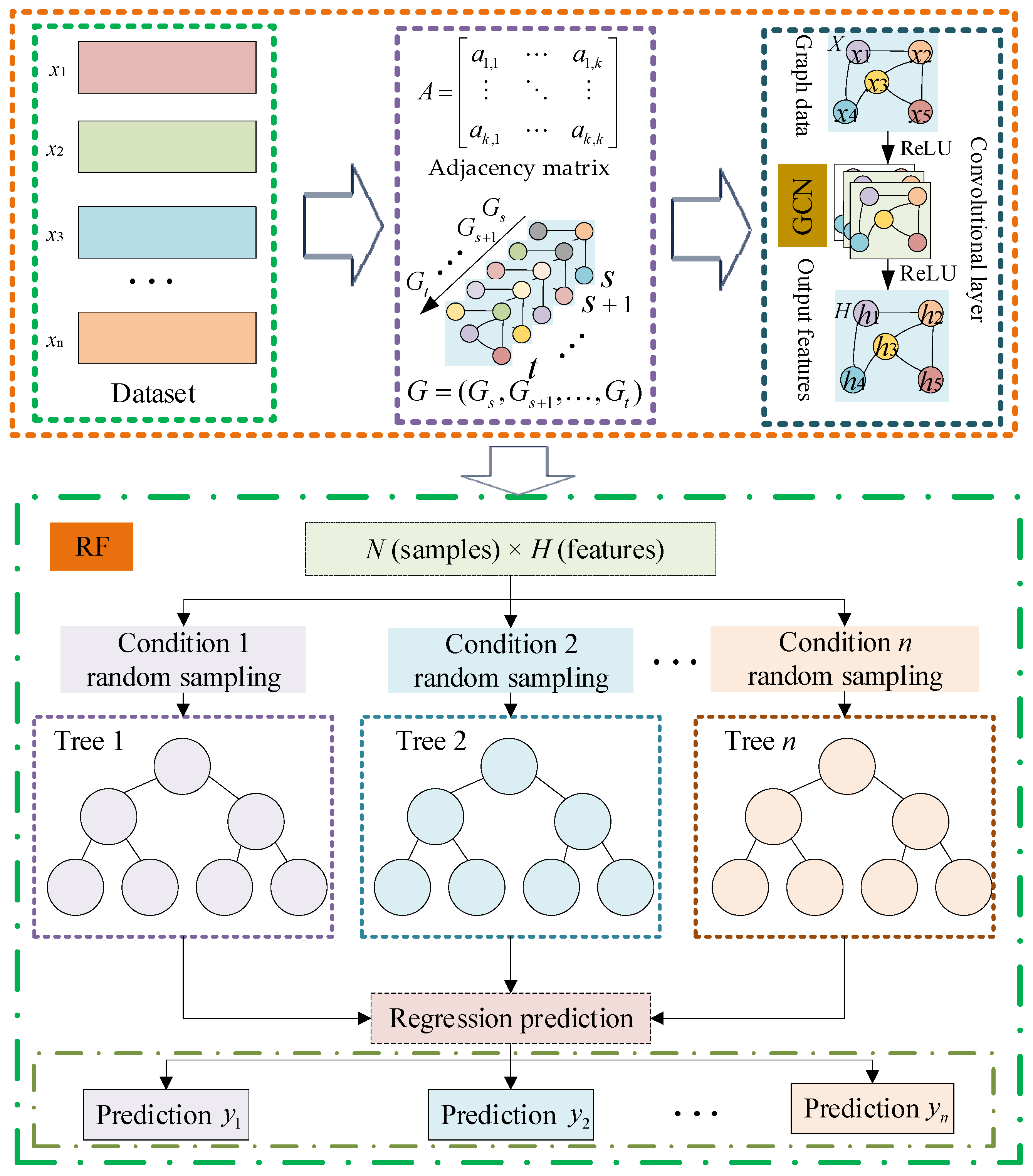
The graph convolutional network (GCN) is a type of deep learning model that extends convolution operations to data structured as graphs. It has shown effective feature extraction abilities when dealing with non-Euclidean data and is widely used in various fields such as social network analysis, recommendation systems, industrial equipment monitoring, and predicting molecular structures [30,31,32]. The main idea is to learn representations of nodes by performing convolution operations on graph data, which helps in capturing relationships between nodes and local structural details efficiently [33]. The basic concept is depicted in Figure 1.
GCN primarily involves key components such as graph structure, adjacency matrix, node features, and convolution operation, as follows.
G = ( V , E )
H ( l + 1 ) = σ ( D ˜ 1 2 A ˜ D ˜ 1 2 H ( l ) W ( l ) )
A ˜ = A + I
D ˜ i i = j A ˜ i j
where V represents the node set; E represents the edge set; A represents the adjacency matrix; A ˜ contains the adjacency matrix with self-loops included for each node; D ˜ is the degree matrix of A ˜ , where the diagonal elements represent the degree of each node, including self-loops; H ( l ) is the node feature matrix of the l-th layer, with H ( 0 ) being the original node feature matrix; W ( l ) is the node feature matrix of the l-th layer; and σ is a non-linear activation function like ReLU.

2.2. Principles of RF

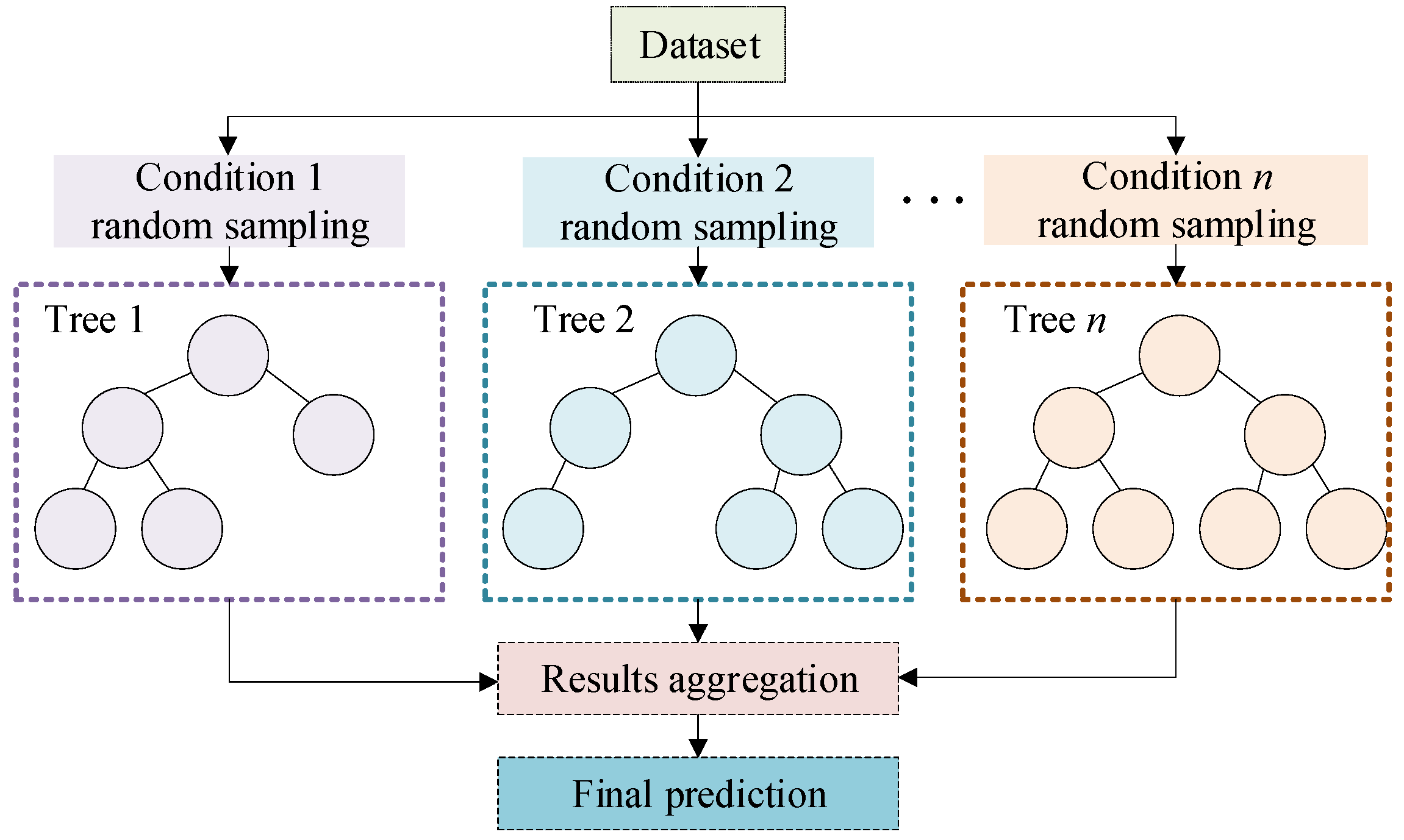
Random forest (RF) is a popular ensemble learning technique that utilizes decision trees and is commonly applied in various areas such as classification, regression, feature selection, and anomaly detection [34,35]. By creating multiple decision trees and aggregating their predictions, RF enhances the model’s accuracy and resilience. Each decision tree in RF is built by randomly selecting data samples and features during training [36]. The fundamental concept of RF is illustrated in Figure 2.

2.3. GCN–RF Model

The GCN–RF combination approach leverages the strengths of both methods. GCN is utilized to extract significant correlation features from graph structure data, while RF employs these features to make regression predictions, as shown in Figure 3.

2.3.1. GCN Structure Design

The design of the GCN network structure needs to consider the number of graph convolution layers, the number of nodes in each layer, and the activation function.
(1) Input layer: Input node feature matrix X and adjacency matrix A. The node feature matrix X contains the standardized data of each sensor node.
(2) Hidden layer: Multiple layers of graph convolution layers can be stacked, and each layer calculates new node features through a formula. The number of nodes in each layer can be selected according to the complexity of the task and the size of the data.
(3) Output layer: The last graph convolution layer outputs a new node feature matrix, which contains the final feature representation of each node.
(4) Activation function: Apply an activation function (such as ReLU) after each layer of graph convolution operation to introduce nonlinearity.

2.3.2. RF Structure Design

(1) Input features: The input features of RF are the node feature matrix H extracted by GCN.
(2) Number of decision trees: The number of decision trees in RF is a key parameter, usually being 100 to 500 trees. More decision trees can improve the stability of the model, but also increase the computational complexity.
(3) Other parameters: These include parameters such as maximum tree depth, minimum number of sample splits, and minimum number of leaf nodes, which need to be optimized through cross-validation.

2.3.3. Multi-Output Regression Prediction

The features extracted by GCN are input into the random forest for multi-output variable prediction. For each node i, whose feature is h, it is input into the random forest model for multi-output variable prediction, as shown in Formula (5).
Y ^ i , m = 1 B b = 1 B T b , m ( h i )
where Y ^ i , m is the predicted result of the m-th output variable of node i.

2.3.4. Performance Evaluation Indicators

To comprehensively evaluate the performance of the model, we use the following evaluation indicators [37].
(1) Coefficient of determination (R2): It reflects the explanatory power of the model, with a value range of [0, 1]. The larger the value, the better the model, as shown in Formula (6).
R 2 = 1 i = 1 n ( y i y ^ i ) 2 i = 1 n ( y i y ¯ ) 2
(2) Mean square error (MSE): It measures the average value of the square error between the predicted value and the actual value, as shown in Formula (7).
M S E = 1 n i = 1 n ( y i y ^ i ) 2
(3) Root mean square error (RMSE): It measures the difference between the predicted value and the actual value, as shown in Formula (8).
R M S E = M S E

3. Case Studies: Truck Crane Operating System

3.1. Principle of Hydraulic Systems of Truck Crane

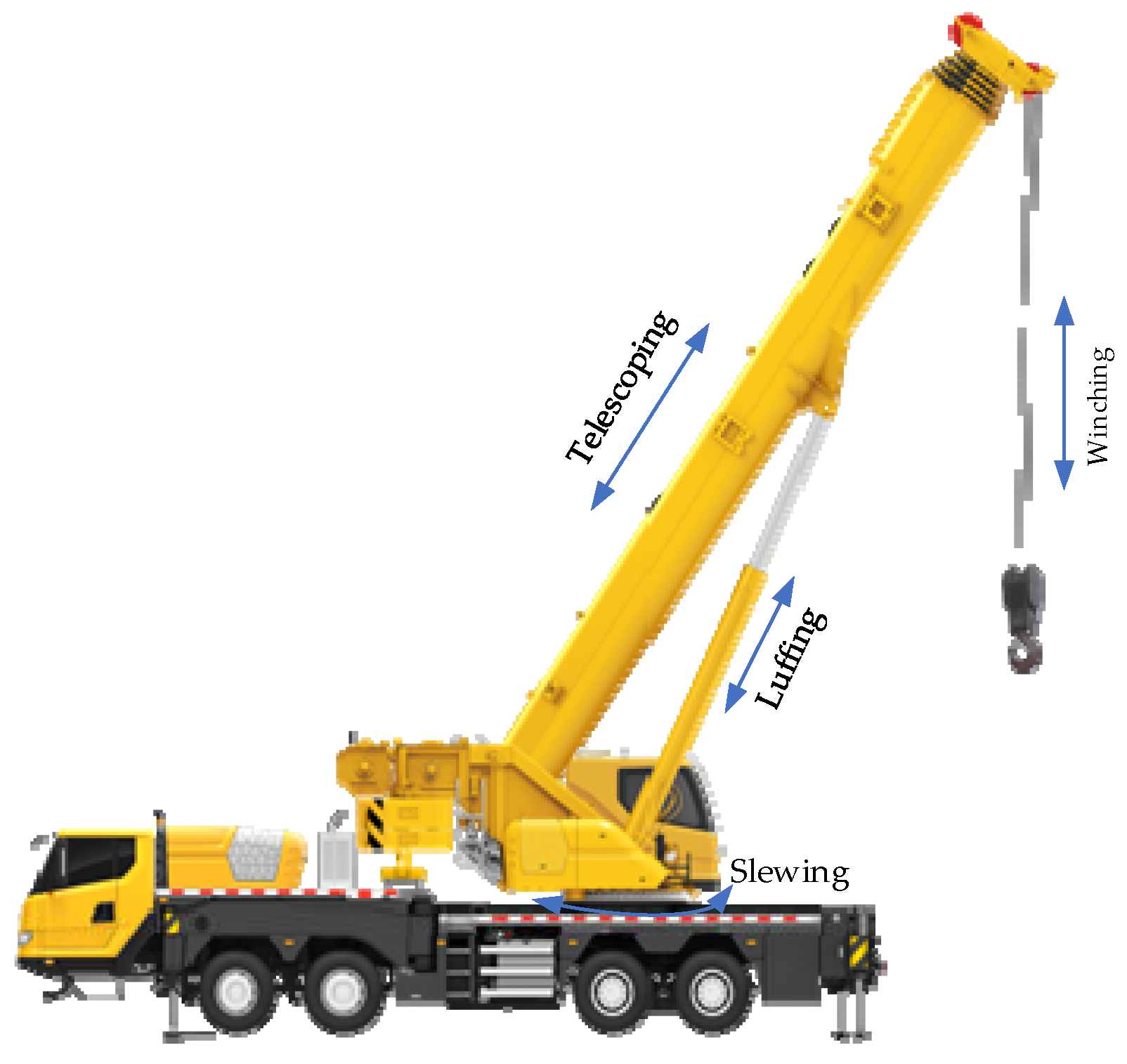
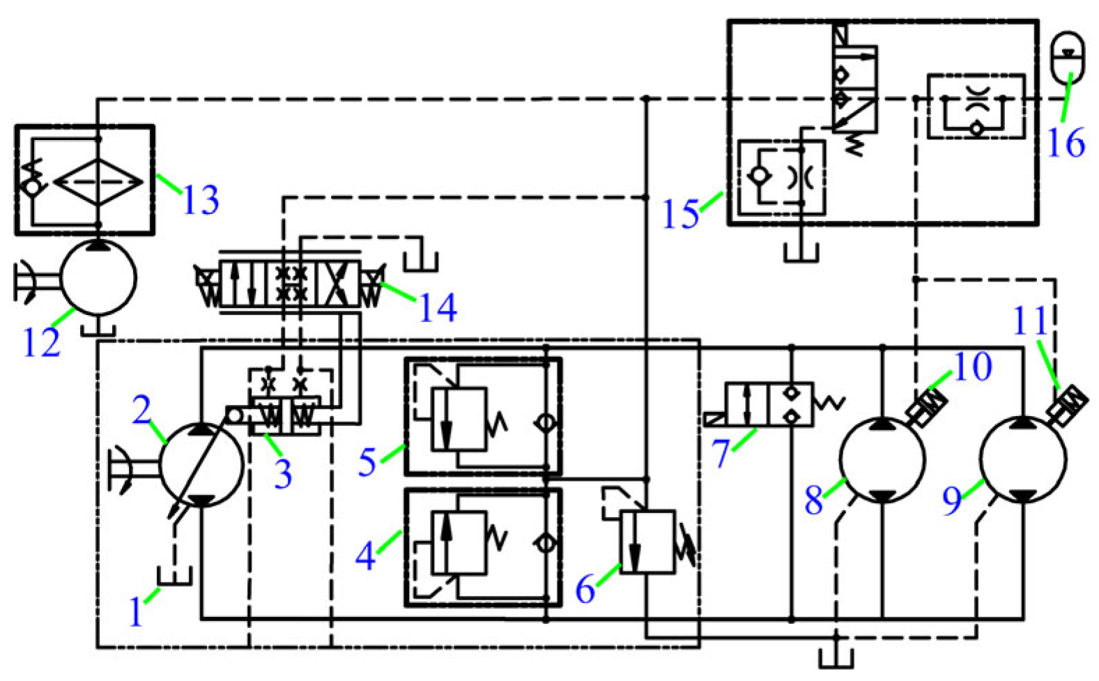
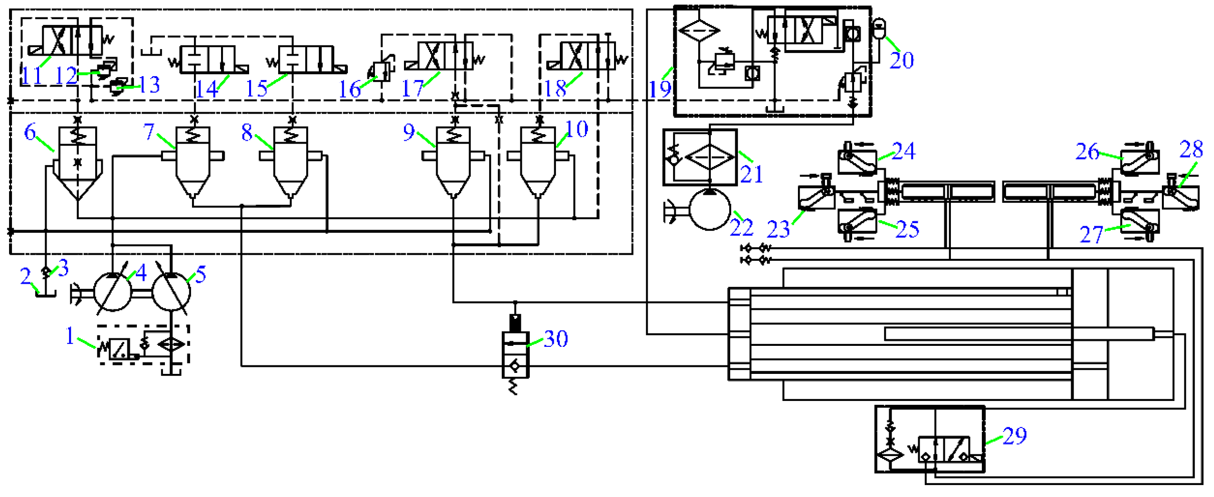
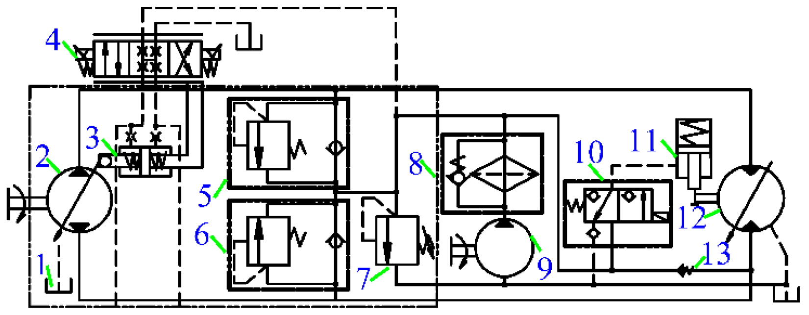
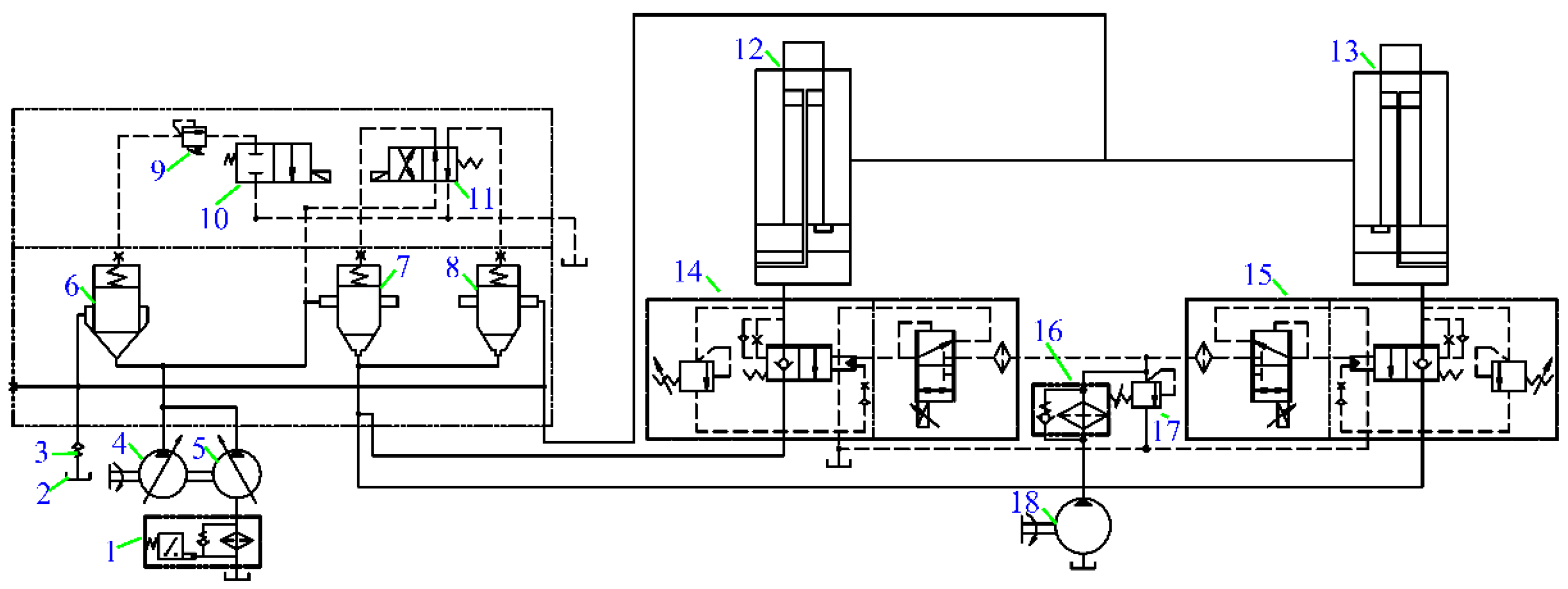
The dataset used in this experiment is derived from actual operational data from a truck crane, which consist of the luffing, telescoping, slewing, and winching systems, as shown in Figure 4. The focus of this study is on the operational performance parameters of crane hydraulic systems. Therefore, hydraulic schematic diagrams for each operational system are provided, as shown in Figure 5, Figure 6, Figure 7 and Figure 8.

3.2. Operation Data Collection

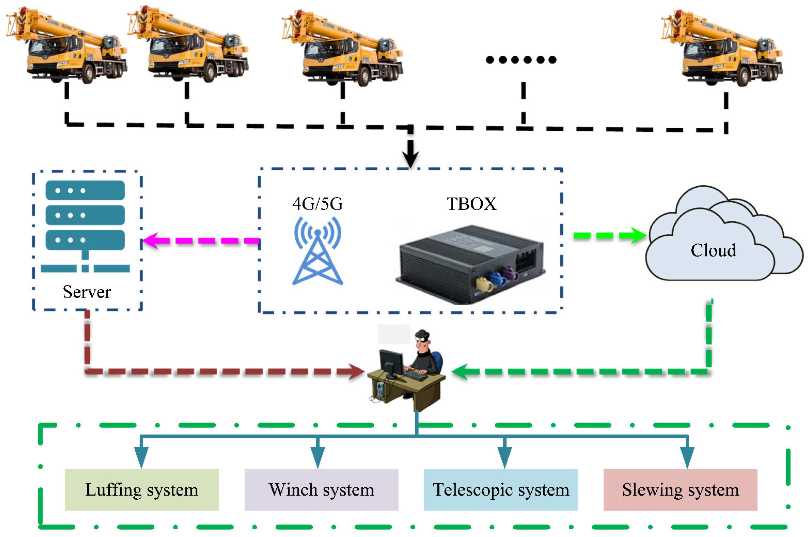
The experimental data in this research are derived from actual crane operation data acquired at the construction site using TBOX. The sampling frequency is set to 1 Hz when the truck cranes leave the factory. Figure 9 shows a data collecting diagram.
Table 1 shows the important variables obtained. Table 2 shows the GCN–RF model parameters.
The x1x16 are the input variables and the y1y8 are the target variables according to the analysis of the truck crane operation mechanism. Three baseline approaches are evaluated for performance analysis using the MIMO soft sensor models, gradient boosting trees (GBTs) [38], support vector regression (SVR) [39], and multi-layer perceptron (MLP) [40]. All these techniques were created using the PyTorch architecture as a foundation. These models are operated on a server that has an Intel i7-9700 3.00 GHz CPU, an NVIDIA Geforce GTX 1050 Ti, and 16 GB of RAM, running Windows 10 [41].
We collected operational data from three cranes with lifting capacities of 160 t, 200 t, and 240 t under actual working conditions. Each dataset is divided into a training set and a test set, with a ratio of 8:2. Real-world operations for truck cranes frequently involve both single and compound actions under varying working conditions. To make predictions, we therefore chose crucial factors in each system that are extremely important. Winch speed, winch pump outlet pressure, slewing angle, boom length, flexible pump pressure, luffing angle, amplitude, and height are the eight main variables that are included in the analysis, along with their respective forecast findings and accuracy. Due to the different dimensions of the collected variables, we need to normalize the data to map them within the range [0, 1], as shown in Formula (9).
x = x x min x max x min
where x is the original value, x is the normalized value, x min is the minimum value in the dataset, and x max is the maximum value in the dataset.
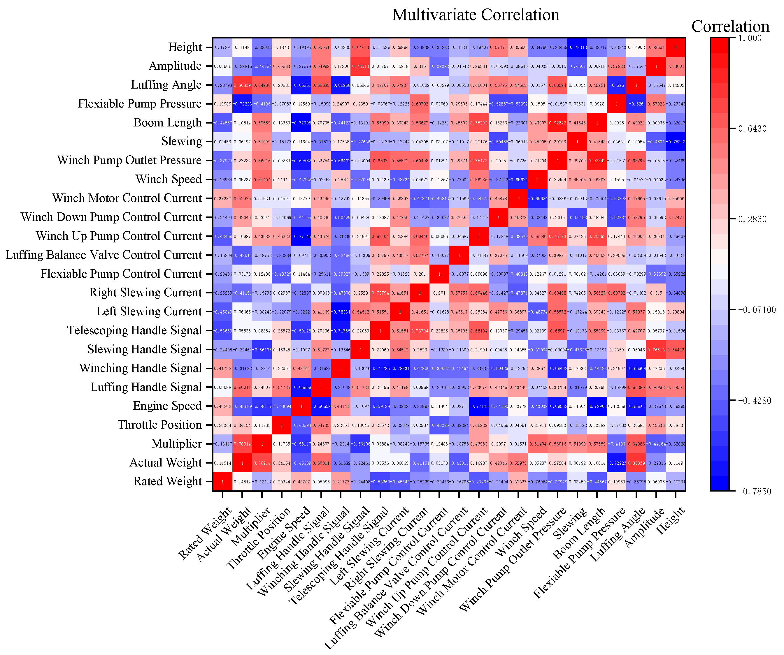
The correlation between variables was analyzed based on data from the actual operating conditions of the crane, identifying input variables that are strongly correlated with the target variables, as shown in Figure 10.
The analysis of Figure 10 reveals the correlation between the target variables of amplitude, boom length, flexible pump pressure, height, luffing angle, slewing angle, winch pump outlet pressure, and winch speed with the input variables, as detailed below.
(1)
A significant correlation exists between amplitude and both the luffing handle signal and the luffing balance valve control current. In contrast, the correlation with variables such as rated weight, actual weight, throttle position, and engine speed is comparatively weaker or not statistically significant.
(2)
A notable positive correlation exists between boom length and both the telescoping handle signal and the luffing handle signal. Conversely, the relationships between boom length and variables such as rated weight, actual weight, throttle position, and engine speed are either weak or not statistically significant.
(3)
The flexible pump pressure exhibits a notable positive correlation with several variables, including flexible pump control current, telescoping handle signal, luffing balance valve control current, and winch up pump control current. Conversely, variables such as slewing handle signal, left slewing current, and right slewing current demonstrate a weaker or negligible correlation with flexible pump pressure.
(4)
The data indicate a positive correlation between height and the luffing handle signal, telescoping handle signal, and luffing balance valve control current. In contrast, the correlation between height and other variables, such as rated weight, engine speed, and winch, is comparatively weaker or not statistically significant.
(5)
The luffing angle exhibits a positive correlation with the luffing handle signal, the control current of the luffing balance valve, and the telescoping handle signal. In contrast, its correlation with variables such as rated weight, engine speed, and winch is comparatively weaker or not statistically significant.
(6)
The slewing angle exhibits a robust positive correlation with the slewing handle signal, left slewing current, and right slewing current. Conversely, variables such as Rated weight, engine speed, and flexible pump control current demonstrate a weaker correlation or lack significant association with the slewing angle.
(7)
The analysis reveals a positive correlation between winch pump outlet pressure and several winch-related control currents, specifically winch motor control current, winch up pump control current, winch down pump control current, and winching handle signal. In contrast, the correlation between winch pump outlet pressure and other variables, including flexible pump control current, slewing handle, left slewing current, and right slewing current, is comparatively weaker.
(8)
The analysis reveals a positive correlation between winch speed and several variables, including engine speed, winch motor control current, winch up pump control current, winching handle signal, and winch down pump control current. In contrast, the correlation between winch speed and variables such as left slewing current, right slewing current, and flexible pump control current is comparatively weaker.

3.3. Key Variables Prediction Results of the 160 t Truck Crane

The prediction results of the amplitude are shown in Figure 11 and the R2, MSE, and RMSE of GCN–RF, GBT, SVR, and MLP are shown in Table 3.
Figure 11 illustrates a comparison between the actual and predicted values of the GCN–RF, GBT, SVR, and MLP in predicting amplitude. The prediction curve produced by the GCN–RF demonstrates a close correspondence with the actual curve, indicating a high level of predictive accuracy. Notably, the GBT’s prediction curve aligns well with the actual values, exhibiting only minor deviations in specific areas attributed to volatility. In contrast, the prediction curves for the SVR and MLP reveal substantial discrepancies from the actual values, particularly in regions marked by rapid fluctuations. This suggests that the SVR and MLP are less effective in amplitude prediction compared to the GCN–RF and GBT.
Table 3 provides the R2, MSE, and RMSE metrics for each model. The GCN–RF achieves the highest R2 value of 0.8875, indicating its excellent explanatory power and fitting capability. Its MSE and RMSE values are 0.0031 and 0.0556, respectively, which are the lowest among the models, highlighting the GCN–RF’s exceptional accuracy in amplitude prediction. The GBT presents an R2 value of 0.8680, an MSE of 0.0036, and an RMSE of 0.0603, demonstrating strong predictive performance. In contrast, the SVR exhibits an R2 value of 0.6116, an MSE of 0.0108, and an RMSE of 0.1039, indicating average performance in amplitude prediction with relatively lower accuracy. Lastly, the MLP records the lowest R2 value of 0.6329, along with an MSE of 0.0101 and an RMSE of 0.1007, reflecting greater prediction errors and inconsistent performance.
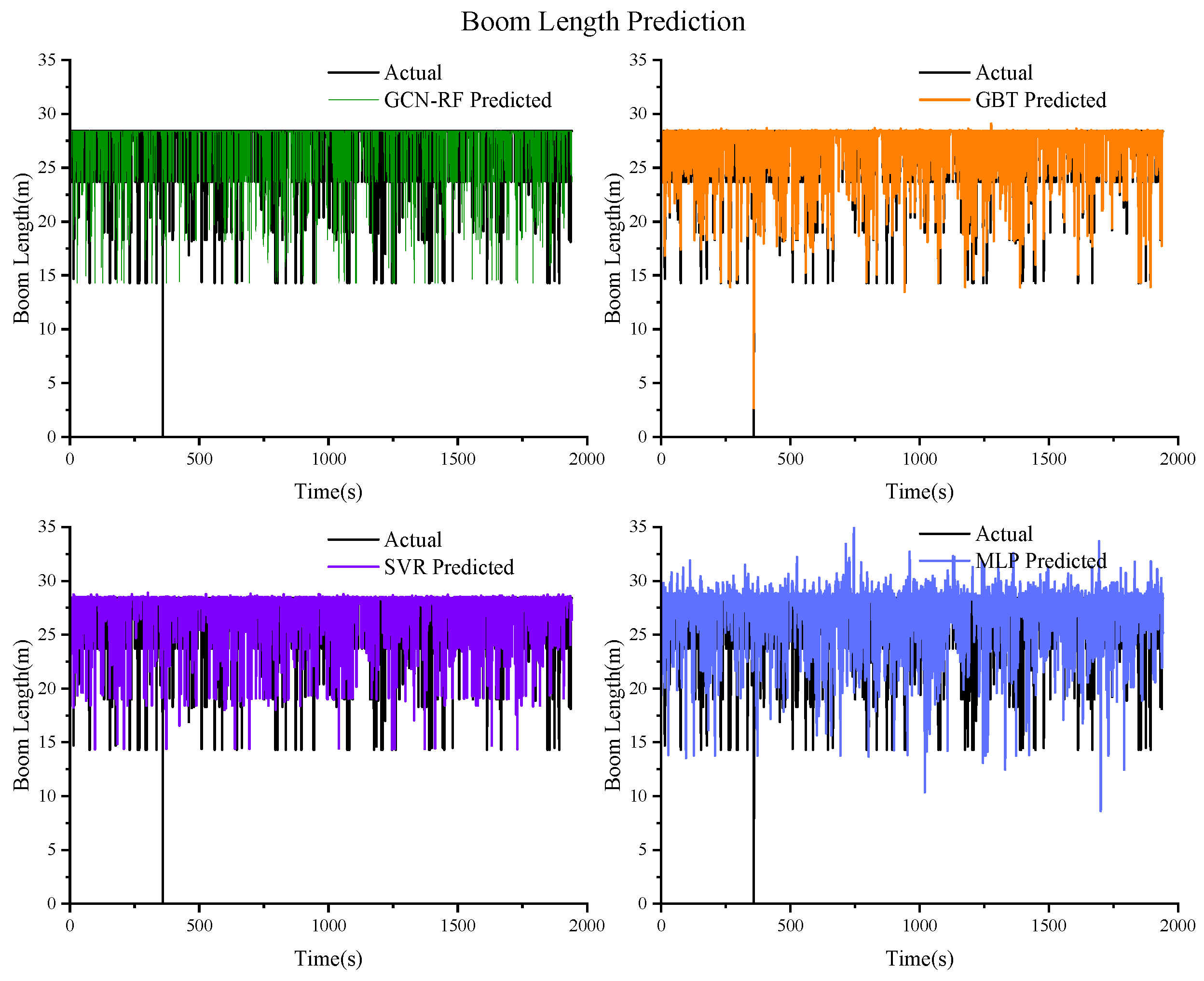
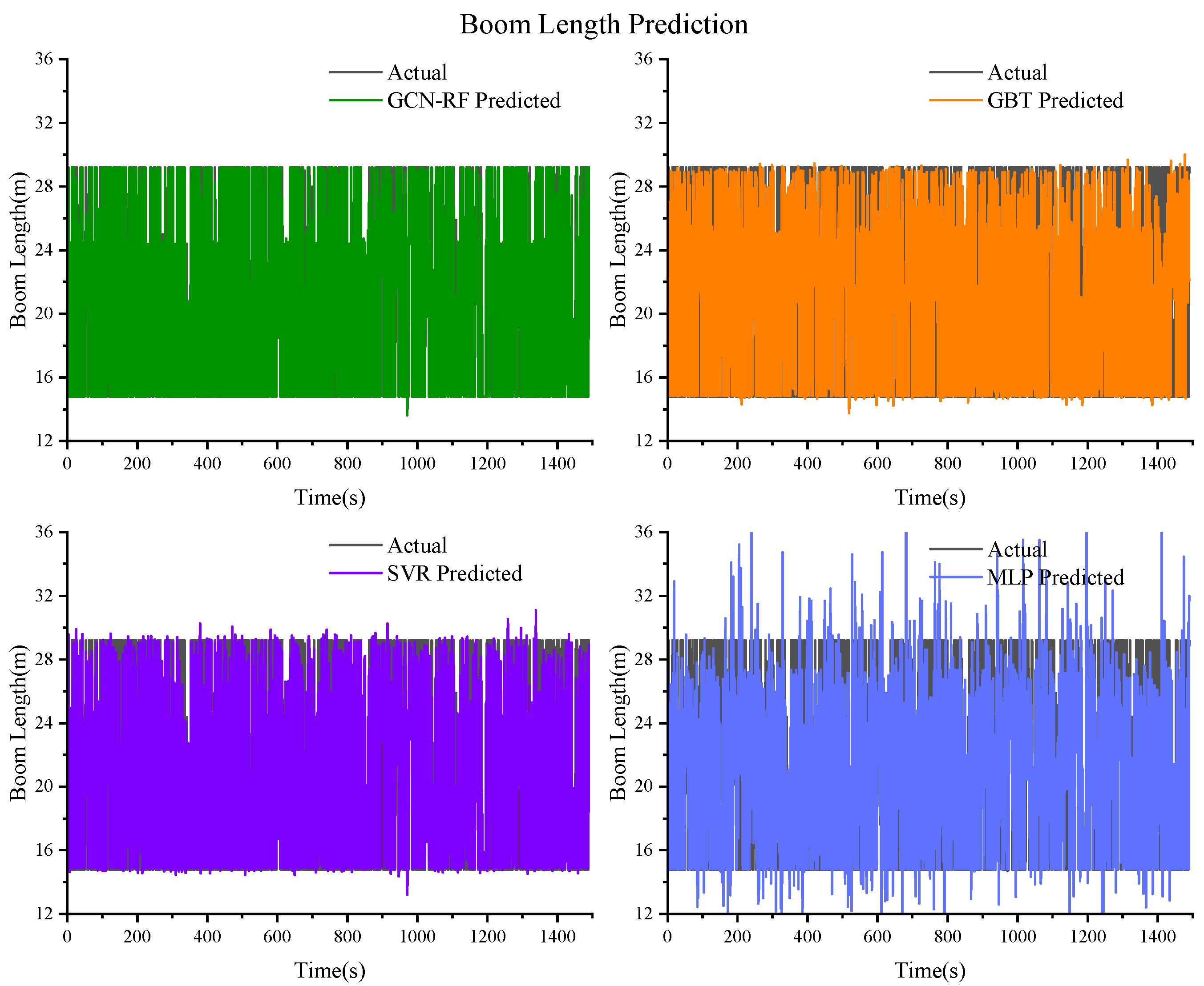
The prediction results of the boom length are shown in Figure 12 and the R2, MSE, and RMSE of GCN–RF, GBT, SVR, and MLP are shown in Table 4.
Figure 12 illustrates a comparison between the actual and predicted values of the GCN–RF, GBT, SVR, and MLP in predicting boom length. It is evident that the prediction curves for the GCN–RF and GBT closely align with the actual curve, indicating a high level of predictive accuracy. Notably, the GCN–RF’s curve nearly perfectly matches the actual values. In contrast, the SVR’s prediction curve exhibits some deviations from the actual values, particularly in regions with significant data fluctuations. The MLP shows relatively poor performance, as indicated by a larger gap between its prediction curve and the actual values, suggesting a weaker capability in predicting boom length.
Table 4 provides the R2, MSE, and RMSE metrics for each model. The GCN–RF exhibits the highest R2 value of 0.8946, indicating superior performance in terms of explanatory power and fitting ability. The MSE and RMSE values for this model are 0.0014 and 0.0380, respectively, both of which are the lowest among the models, further confirming the exceptional accuracy of the GCN–RF in predicting arm length. The GBT presents an R2 value of 0.8904, an MSE of 0.0014, and an RMSE of 0.0379, also demonstrating strong predictive capability. In contrast, the SVR has an R2 value of 0.6372, an MSE of 0.0082, and an RMSE of 0.0906, indicating significantly poorer performance compared to the GCN–RF and GBT, with lower predictive accuracy. The MLP records the lowest R2 value of 0.5700, with an MSE of 0.0059 and an RMSE of 0.0768, reflecting greater prediction errors and diminished accuracy.
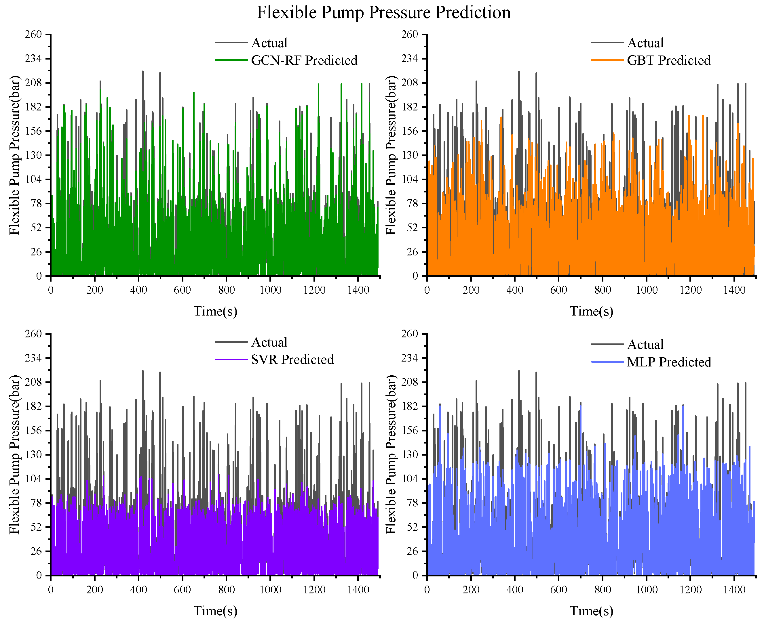
The prediction results of the flexible pump pressure are shown in Figure 13 and the R2, MSE, and RMSE of GCN–RF, GBT, SVR, and MLP are shown in Table 5.
Figure 13 illustrates a comparison between the actual and predicted values of the GCN–RF, GBT, SVR, and MLP in predicting flexible pump pressure. The results indicate that the prediction curve of the GCN–RF closely aligns with the actual curve, thereby indicating a high level of predictive accuracy. The GBT exhibits a similar trend, maintaining consistency with the actual values overall, although it does present some deviations characterized by fluctuations in specific regions. In contrast, the prediction curves for the SVR and MLP reveal more substantial discrepancies from the actual values, particularly in areas experiencing significant pressure variations, suggesting that these models are less effective than the GCN–RF and GBT in predicting flexible pump pressure.
Table 5 provides the R2, MSE, and RMSE metrics for each model. The GCN–RF achieves the highest R2 value of 0.8689, signifying superior performance in terms of explanatory power and fitting capability. The corresponding MSE and RMSE values are 0.0048 and 0.0691, respectively, both of which are the lowest among the models, further substantiating the GCN–RF’s high accuracy in predicting flexible pump pressure. The GBT presents an R2 value of 0.8124, an MSE of 0.0080, and an RMSE of 0.0897, demonstrating commendable predictive capability. Conversely, the SVR exhibits an R2 value of 0.6767, an MSE of 0.0107, and an RMSE of 0.1172, indicating a significantly lower predictive accuracy compared to the GCN–RF and GBT. The MLP records the lowest R2 value of 0.7200, with an MSE of 0.0102 and an RMSE of 0.1010, reflecting greater prediction errors and diminished accuracy.
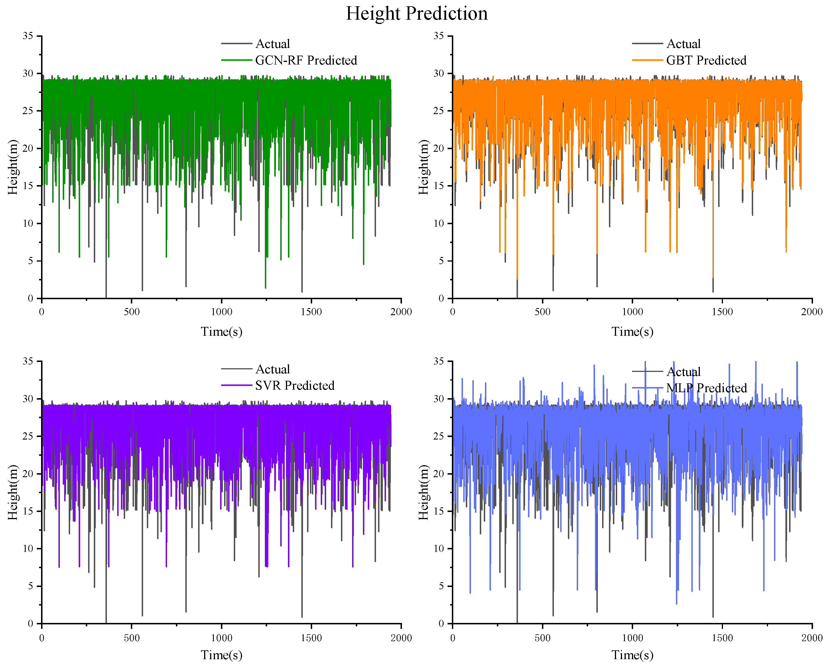
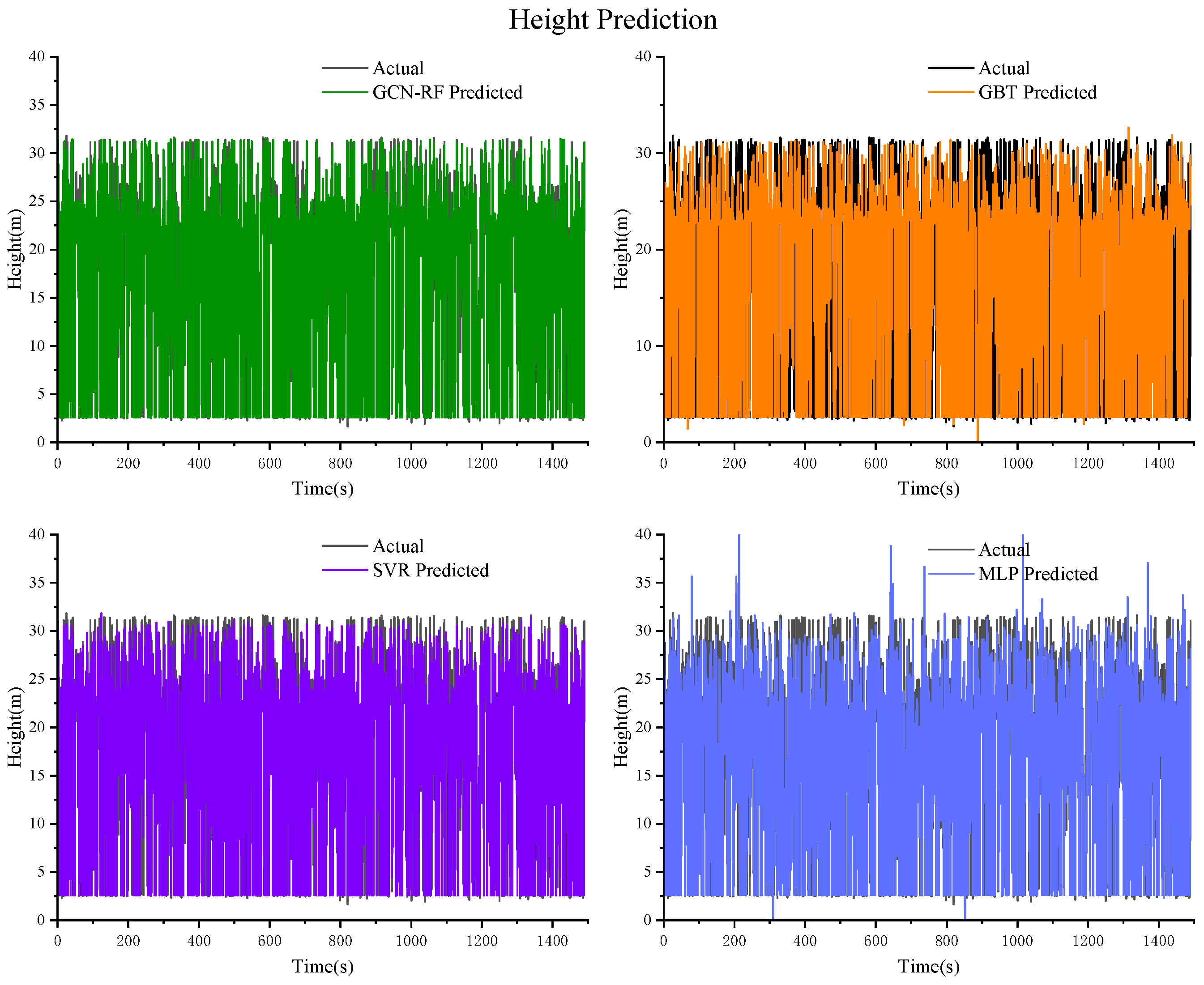
The prediction results of the height are shown in Figure 14 and the R2, MSE, and RMSE of GCN–RF, GBT, SVR, and MLP are shown in Table 6.
Figure 14 illustrates a comparison between the actual and predicted values of the GCN–RF, GBT, SVR, and MLP in predicting height. The prediction curves for the GCN–RF and GBT closely align with the actual curve, indicating a high level of predictive accuracy. Notably, the GBT’s prediction curve nearly coincides with the actual values. Conversely, the prediction curves for the SVR and MLP display more pronounced deviations from the actual values, particularly in regions characterized by significant height variations, suggesting that these models exhibit inferior performance relative to the GCN–RF and GBT in the height prediction.
Table 6 provides the R2, MSE, and RMSE metrics for each model. The GBT achieves the highest R2 value of 0.9260, signifying its exceptional explanatory power and fitting capability. The corresponding MSE and RMSE values are 0.0014 and 0.0374, respectively, both of which are the lowest among the models, thereby reinforcing the GBT’s accuracy in height prediction. The GCN–RF presents an R2 value of 0.9248 and still reflects robust predictive capability accompanied by an MSE of 0.0015 and an RMSE of 0.0388, which are slightly lower values than those of the GBT. In contrast, the SVR exhibits an R2 value of 0.8047, with an MSE of 0.0047 and an RMSE of 0.0669, indicating a significantly lower predictive accuracy compared to the GCN–RF and GBT. The MLP records the lowest R2 value of 0.8312, with an MSE of 0.0036 and an RMSE of 0.0583. Although it marginally outperforms the SVR, it still demonstrates greater prediction errors.
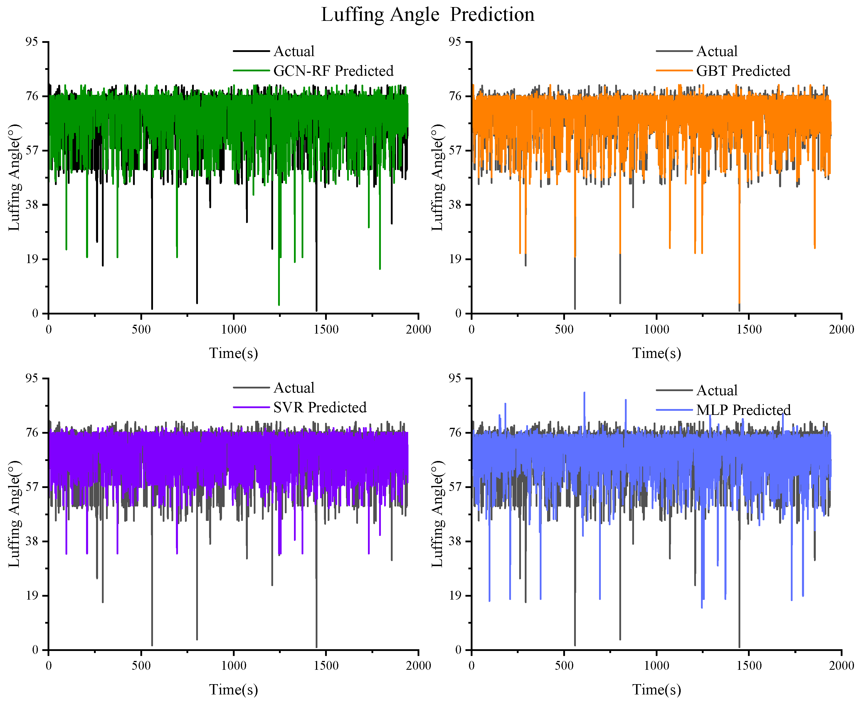
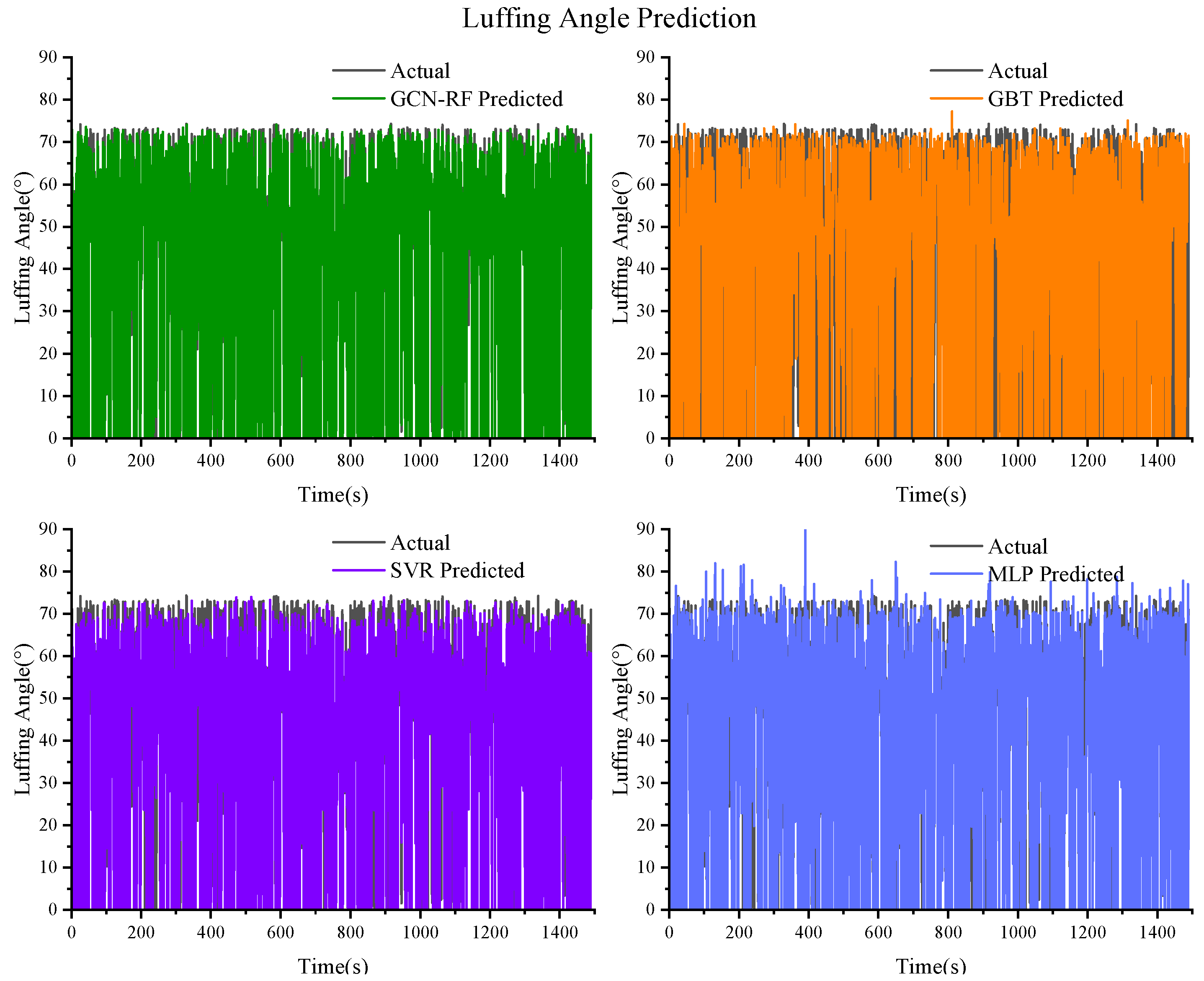
The prediction results of the luffing angle are shown in Figure 15 and the R2, MSE, and RMSE of GCN–RF, GBT, SVR, and MLP are shown in Table 7.
Figure 15 illustrates a comparison between the actual and predicted values of the GCN–RF, GBT, SVR, and MLP in predicting amplitude angle. The results indicate that the prediction curves for the GCN–RF and GBT closely align with the actual curve, signifying a high level of predictive accuracy. Notably, the two curves nearly coincide in regions characterized by stable changes. Conversely, the prediction curves for the SVR and MLP display more pronounced deviations from the actual values, particularly in areas with significant fluctuations, indicating that these models exhibit inferior performance relative to the GCN–RF and GBT in amplitude angle prediction.
Table 7 provides the R2, MSE, and RMSE metrics for each model. The GCN–RF achieves the highest R2 value of 0.8952 among the four models, signifying superior performance in terms of explanatory power and fitting capability. The MSE and RMSE values for this model are 0.0015 and 0.0381, respectively, both of which are the lowest, further corroborating the GCN–RF’s high accuracy in amplitude angle prediction. The GBT presents an R2 value of 0.8917, an MSE of 0.0015, and an RMSE of 0.0384, demonstrating robust predictive capability. In contrast, the SVR exhibits an R2 value of 0.6577, an MSE of 0.0676, and an RMSE of 0.0768, indicating significantly lower predictive accuracy compared to the GCN–RF and GBT models. The MLP records the lowest R2 value of 0.6718, with an MSE of 0.0059 and an RMSE of 0.0767, reflecting greater prediction errors and diminished accuracy.
The prediction results of the slewing angle are shown in Figure 16 and the R2, MSE, and RMSE of GCN–RF, GBT, SVR, and MLP are shown in Table 8.
Figure 16 illustrates a comparison between the actual and predicted values of the GCN–RF, GBT, SVR, and MLP in predicting slewing angle. The prediction curve of the GCN–RF closely aligns with the actual curve, suggesting a high level of predictive accuracy. The GBT still adheres to the overall trend of the observed data while exhibiting some deviation from the actual values. In contrast, the prediction curves for the SVR and MLP display more pronounced discrepancies from the actual values, particularly in regions characterized by significant data fluctuations, thereby indicating inferior performance relative to the GCN–RF and GBT in the task of slewing angle prediction.
Table 8 provides the R2, MSE, and RMSE metrics for each model. The GCN–RF achieves the highest R2 value of 0.8752 among the four models, signifying superior performance in terms of explanatory power and fitting capability. The MSE and RMSE values for this model are 0.0053 and 0.0728, respectively, both of which are the lowest recorded, further substantiating the GCN–RF’s high accuracy in slewing angle prediction. The GBT presents an R2 value of 0.7975, an MSE of 0.0089, and an RMSE of 0.0944. Although it is slightly less accurate than the GCN–RF, it still demonstrates commendable predictive capability. Conversely, the SVR exhibits an R2 value of 0.5463, an MSE of 0.0193, and an RMSE of 0.1390, indicating significantly poorer performance when compared to the GCN–RF and GBT, along with reduced predictive accuracy. The MLP records the lowest R2 value of 0.5220, with an MSE of 0.0203 and an RMSE of 0.1423, reflecting greater prediction errors and diminished accuracy.
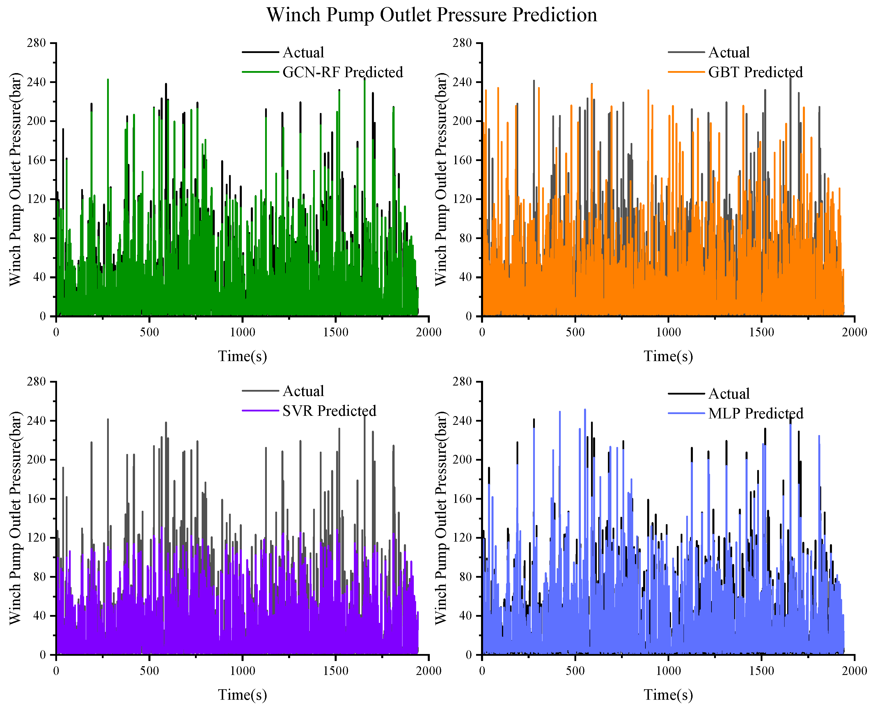
The prediction results of the winch pump outlet pressure are shown in Figure 17 and the R2, MSE, and RMSE of GCN–RF, GBT, SVR, and MLP are shown in Table 9.
Figure 17 illustrates a comparison between the actual and predicted values of the GCN–RF, GBT, SVR, and MLP in predicting winch pump outlet pressure. The prediction curve for the GCN–RF closely aligns with the actual curve, signifying a high level of predictive accuracy. The GBT also demonstrates commendable performance. However, it exhibits noticeable deviations in certain regions characterized by significant fluctuations when compared to the GCN–RF. In contrast, the prediction curves for the SVR and MLP reveal more substantial discrepancies from the actual values, particularly under conditions of heightened data variability, thereby indicating inferior performance relative to the GCN–RF and GBT in the prediction of winch pump outlet pressure.
Table 9 provides the R2, MSE, and RMSE metrics for each model. The GCN–RF achieves the highest R2 value of 0.8948 among the four models, signifying superior performance in terms of explanatory power and fitting capability. The MSE and RMSE values for the GCN–RF are 0.0031 and 0.0555, respectively, both of which are the lowest, further substantiating the model’s high accuracy in predicting winch pump outlet pressure. The GBT presents an R2 value of 0.8089, with an MSE of 0.0068 and an RMSE of 0.0826, demonstrating robust predictive capability. Conversely, the SVR exhibits an R2 value of 0.6917, an MSE of 0.0114, and an RMSE of 0.1070, indicating significantly poorer performance in comparison to the GCN–RF and GBT, along with diminished predictive accuracy. The MLP records the lowest R2 value of 0.7216, accompanied by an MSE of 0.0094 and an RMSE of 0.0997, reflecting greater prediction errors and reduced accuracy.
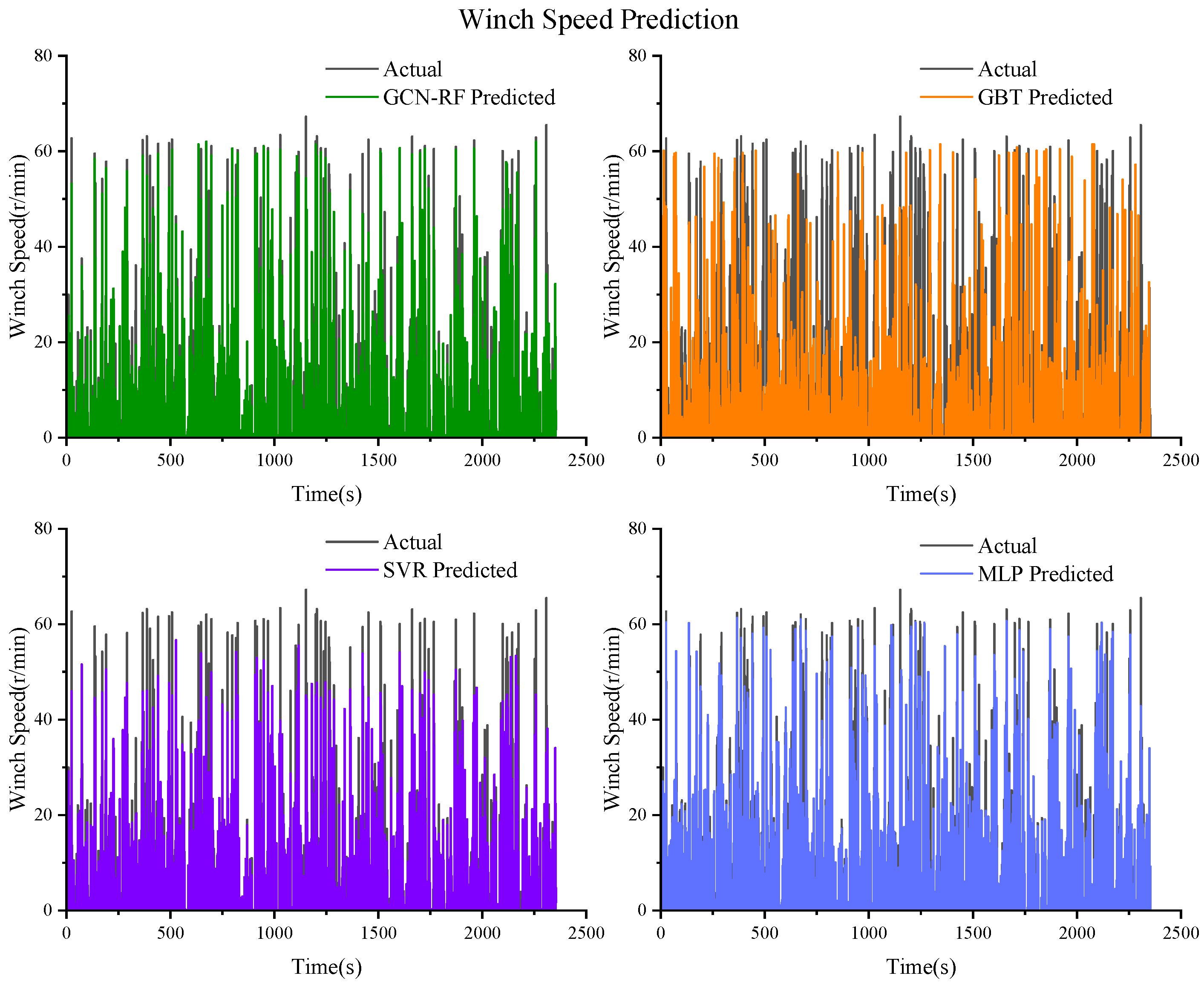
The prediction results of the winch speed are shown in Figure 18 and the R2, MSE, and RMSE of GCN–RF, GBT, SVR, and MLP are shown in Table 10.
Figure 18 illustrates a comparison between the actual and predicted values of the GCN–RF, GBT, SVR, and MLP in predicting winch speed. The prediction curves for the GCN–RF and GBT closely align with the actual data, suggesting a high level of predictive accuracy. Notably, the prediction curve of the GCN–RF nearly coincides with the actual values. Conversely, the prediction curves for the SVR and MLP models exhibit considerable divergence from the actual values, particularly in areas characterized by significant fluctuations in speed, indicating inferior performance in winch speed prediction relative to the GCN–RF and GBT.
Table 10 provides the R2, MSE, and RMSE metrics for each model. The GCN–RF achieves the highest R2 value of 0.9462 among the four models, signifying superior explanatory power and fitting capability. Its MSE and RMSE values are 0.0010 and 0.0323, respectively, both of which are the lowest, further substantiating the GCN–RF’s high accuracy in winch speed prediction. The GBT presents an R2 value of 0.9423, an MSE of 0.0013, and an RMSE of 0.0351, demonstrating commendable predictive performance. In contrast, the SVR exhibits an R2 value of 0.8740, an MSE of 0.0031, and an RMSE of 0.0553, indicating significantly diminished performance compared to the GCN–RF and GBT, with reduced predictive accuracy. The MLP records the lowest R2 value of 0.9176, alongside an MSE of 0.0016 and an RMSE of 0.0400. Although it performs slightly better than the SVR model, it still demonstrates greater prediction errors.

3.4. Key Variables Prediction Results of the 200 t Truck Crane

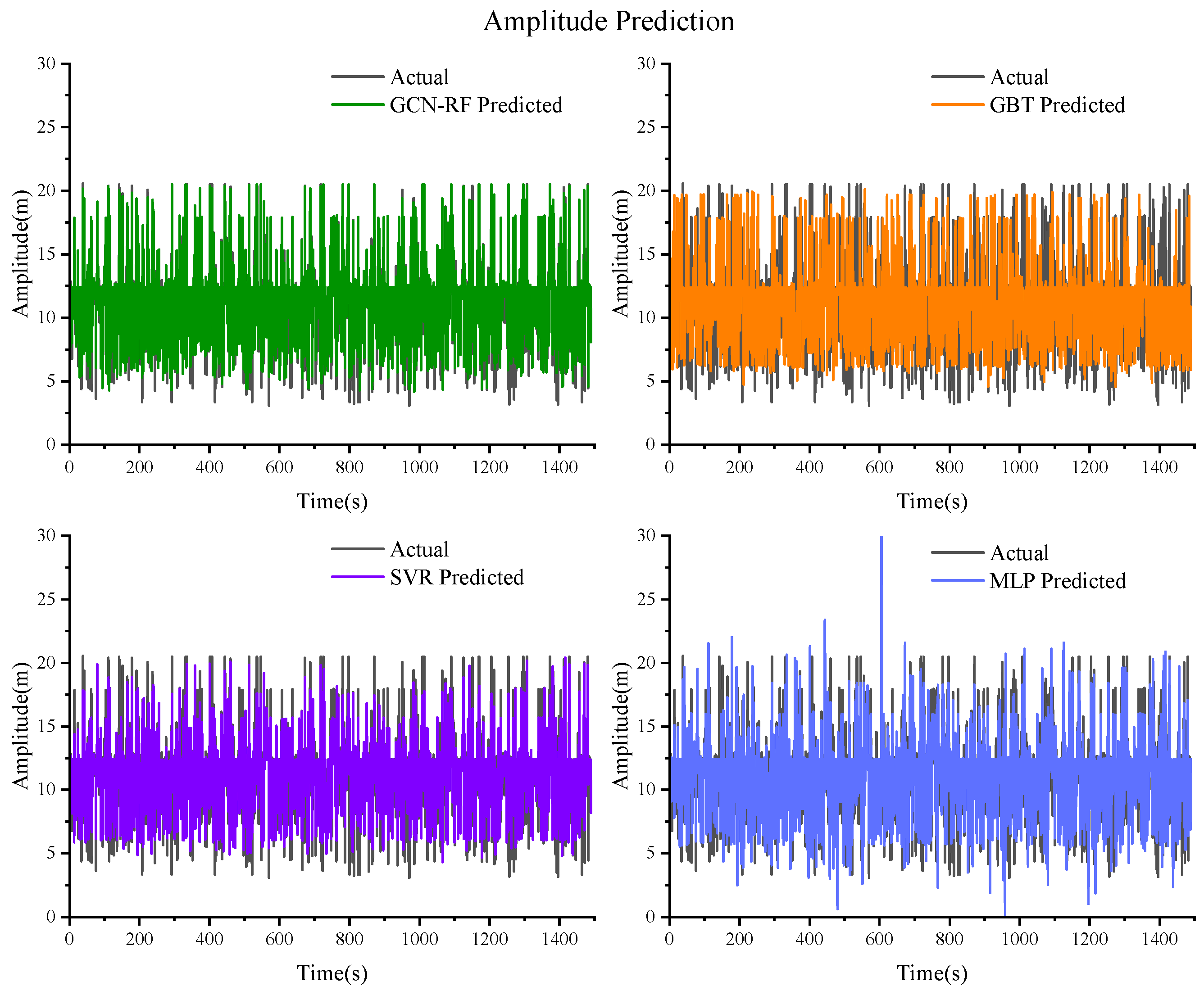
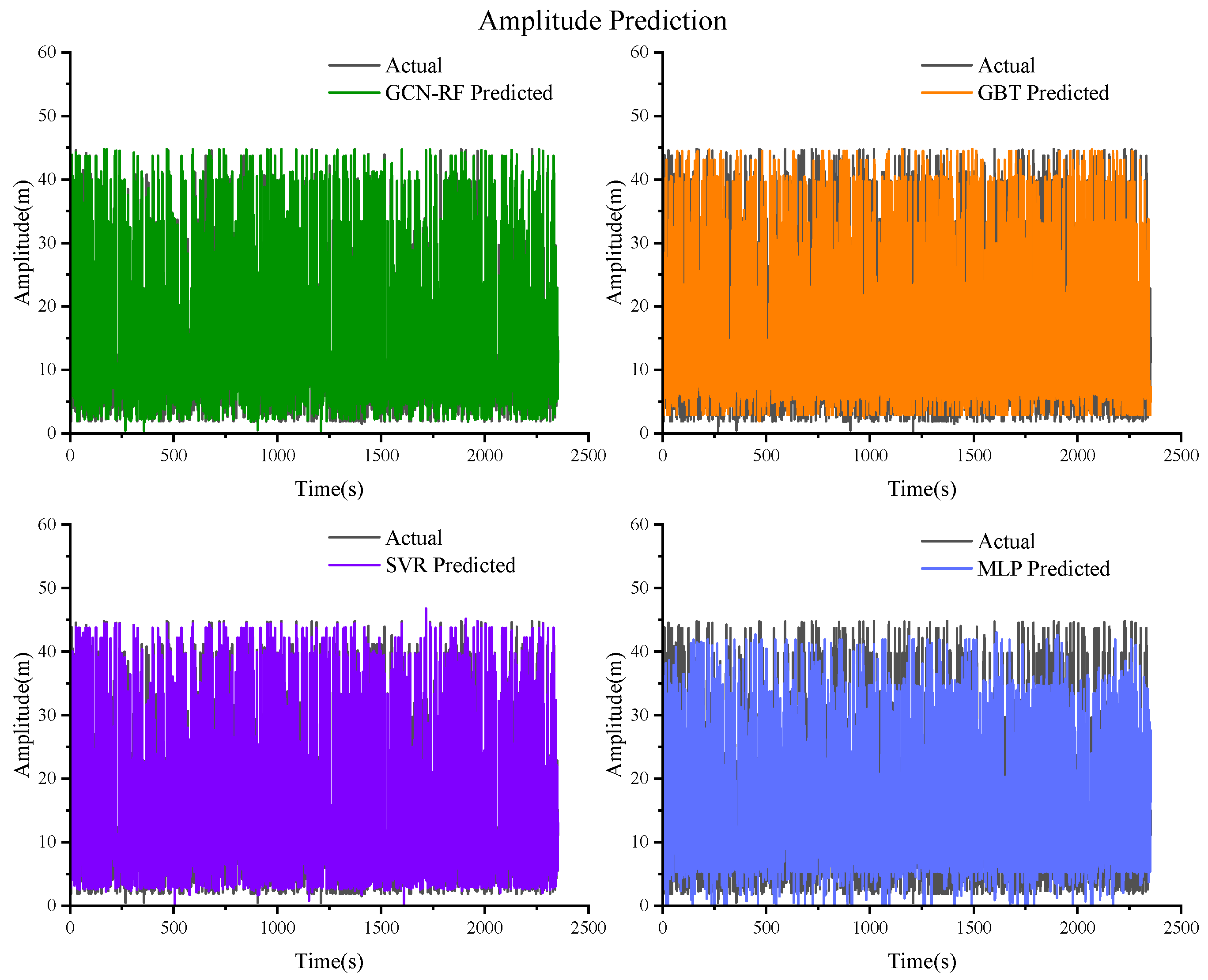
The prediction results of the amplitude are shown in Figure 19 and the R2, MSE, and RMSE of GCN–RF, GBT, SVR, and MLP are shown in Table 11.
Figure 19 illustrates a comparison between the actual and predicted values of the GCN–RF, GBT, SVR, and MLP in predicting amplitude. The results indicate that the prediction curve of the GCN–RF closely approximates the actual curve, signifying a high level of predictive accuracy. The GBT’s prediction curve demonstrates a strong alignment with the actual values, albeit with minor discrepancies in certain fluctuating regions. Conversely, the prediction curves for the SVR and MLP exhibit a significant divergence from the actual values, particularly in areas characterized by substantial data variations, thereby indicating inferior performance in amplitude prediction relative to the GCN–RF and GBT.
Table 11 provides the R2, MSE, and RMSE metrics for each model. The GCN–RF achieves the highest R2 value of 0.8875, signifying superior explanatory power and fitting capability. Its MSE and RMSE values are recorded at 0.0031 and 0.0556, respectively, which are the lowest among the models, further substantiating the GCN–RF’s high accuracy in amplitude prediction. The GBT presents an R2 value of 0.8680, an MSE of 0.0036, and an RMSE of 0.0603, demonstrating commendable predictive performance. In contrast, the SVR exhibits an R2 value of 0.6116, an MSE of 0.0108, and an RMSE of 0.1039, indicating average performance in amplitude prediction with relatively low accuracy. The MLP records the lowest R2 value of 0.6329, an MSE of 0.0101, and an RMSE of 0.1007, reflecting greater prediction errors and a lack of stability in its performance.
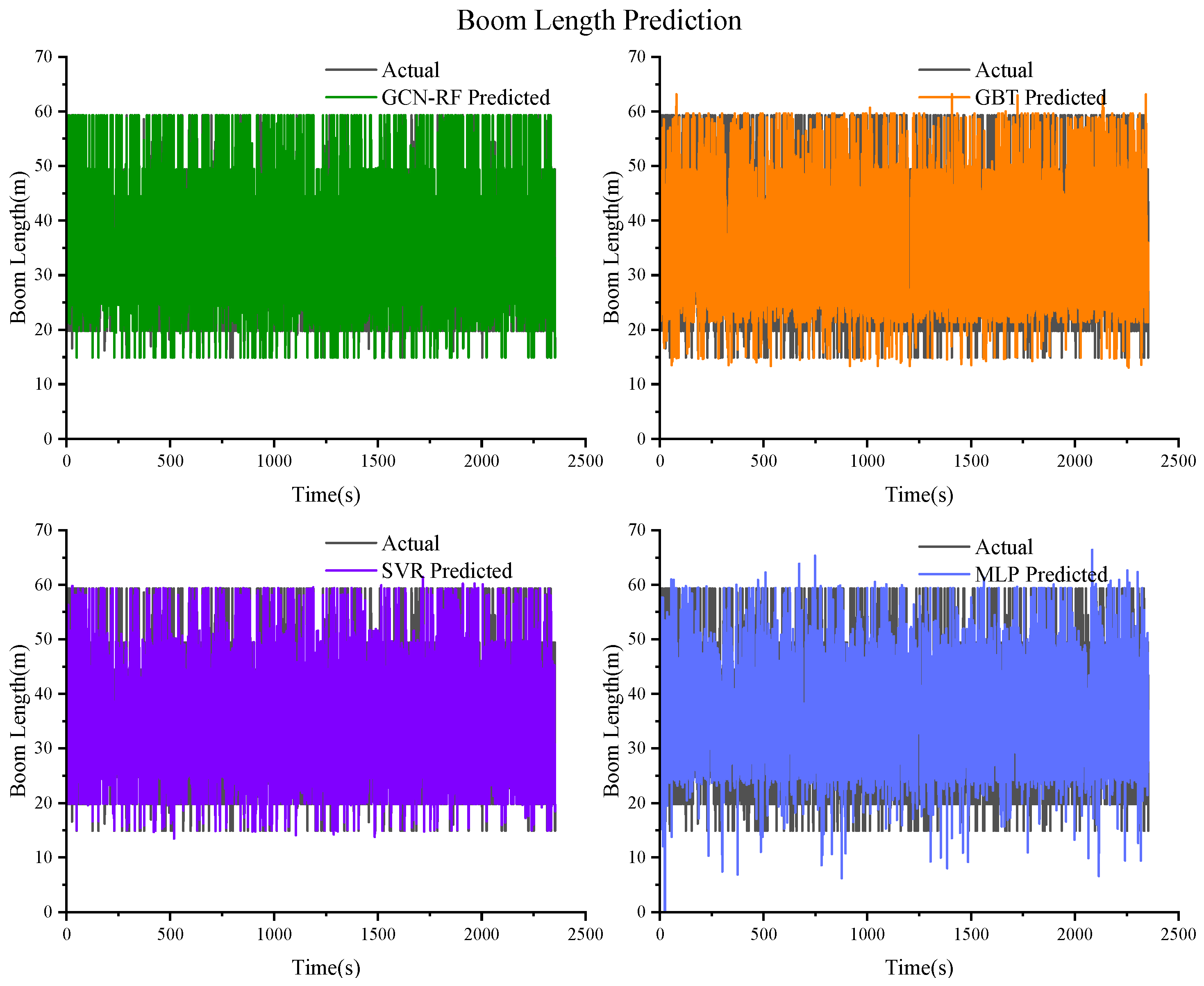
The prediction results of the boom length are shown in Figure 20 and the R2, MSE, and RMSE of GCN–RF, GBT, SVR, and MLP are shown in Table 12.
Figure 20 illustrates a comparison between the actual and predicted values of the GCN–RF, GBT, SVR, and MLP in predicting boom length. The results indicate that the prediction curves for the GCN–RF and GBT closely align with the actual values, suggesting a high degree of predictive accuracy. Notably, the curve for the GCN–RF nearly coincides with the actual data. In contrast, the SVR exhibits some discrepancies from the actual values, particularly in regions characterized by significant fluctuations in the data. The MLP demonstrates comparatively inferior performance, as evidenced by a more pronounced divergence between its prediction curve and the actual values, indicating a reduced efficacy in boom length prediction.
Table 12 provides the R2, MSE, and RMSE metrics for each model. The GCN–RF achieves the highest R2 value of 0.9263, signifying superior fitting performance in the task of boom length prediction. Its MSE and RMSE values are recorded at 0.0032 and 0.0565, respectively, which are the lowest among the evaluated models, thereby reinforcing the GCN–RF’s advantage in predictive accuracy. The GBT presents an R2 value of 0.9051, an MSE of 0.0042, and an RMSE of 0.0646. While its performance is marginally inferior to that of the GCN–RF, it still demonstrates commendable predictive capability. The SVR exhibits an R2 value of 0.9190, which is slightly superior to that of the GBT. However, its MSE and RMSE values are higher, recorded at 0.0074 and 0.1010, respectively, indicating a deficiency in accuracy. The MLP records the lowest R2 value of 0.8307, with an MSE of 0.0104 and an RMSE of 0.0860, reflecting that it is comparatively less effective in addressing the boom length prediction challenge.
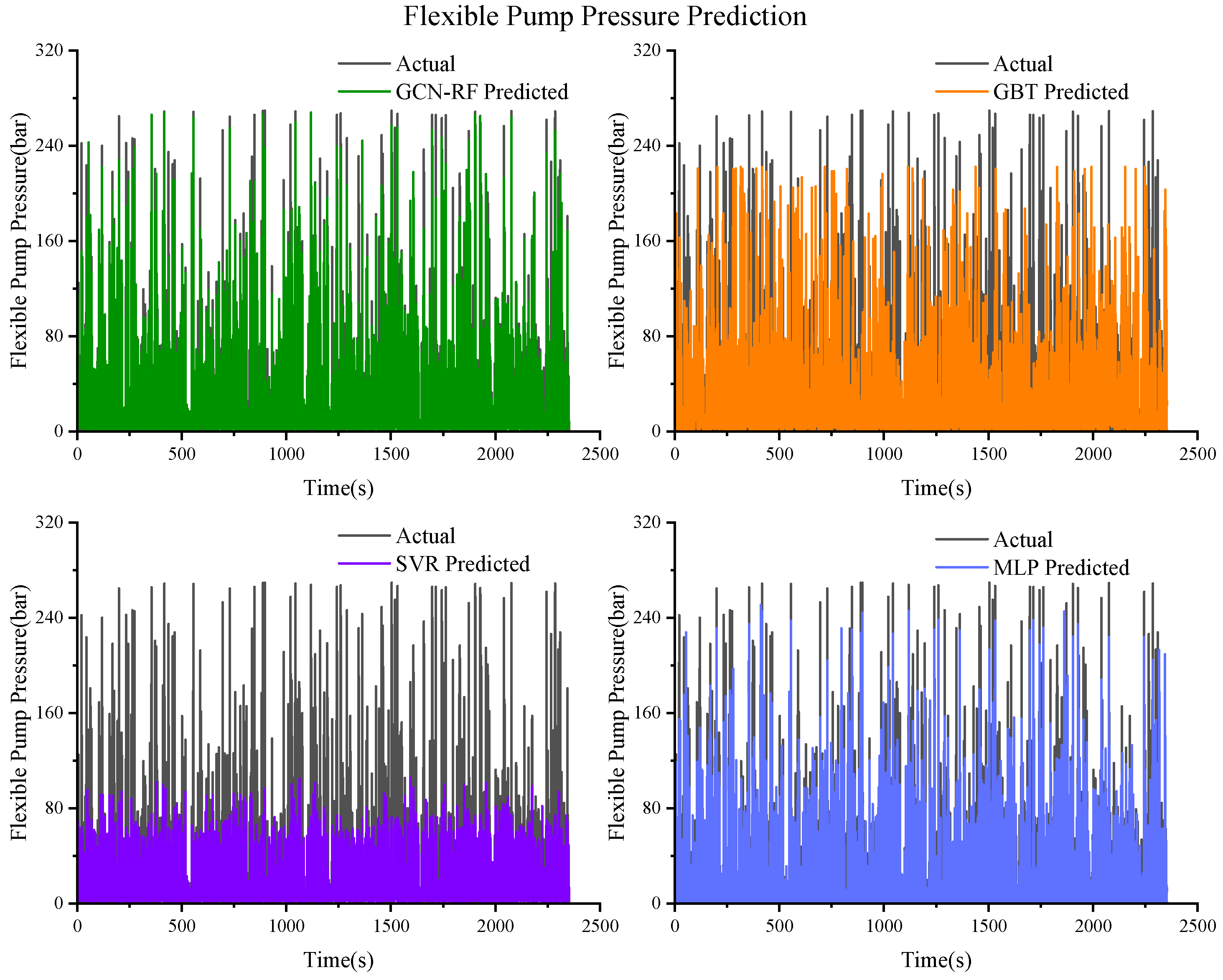
The prediction results of the flexible pump pressure are shown in Figure 21 and the R2, MSE, and RMSE of GCN–RF, GBT, SVR, and MLP are shown in Table 13.
Figure 21 illustrates a comparison between the actual and predicted values of the GCN–RF, GBT, SVR, and MLP in predicting flexible pump pressure. The results indicate that the prediction curve produced by the GCN–RF closely approximates the actual curve, suggesting a high level of predictive accuracy. In contrast, the GBT demonstrates slightly inferior performance; while its predictions generally align with the actual values, there are notable discrepancies in certain fluctuating regions. The prediction curves for the SVR and MLP reveal a considerable divergence from the actual values, particularly in areas characterized by abrupt pressure variations, indicating that these models are less effective in predicting flexible pump pressure when compared to the GCN–RF and GBT.
Table 13 provides the R2, MSE, and RMSE metrics for each model. The GCN–RF achieves the highest R2 value of 0.8769, signifying its superior explanatory power and fitting capability compared to the other models. The corresponding MSE and RMSE values for the GCN–RF are 0.0054 and 0.0733, respectively, both of which are the lowest among the models assessed, further substantiating the GCN–RF’s high accuracy in accuracy for flexible pump pressure prediction. The GBT presents an R2 value of 0.7910, an MSE of 0.0087, and an RMSE of 0.0931, demonstrating a marginally lower performance. The SVR exhibits an R2 value of 0.7218, which is inferior to both the GCN–RF and GBT, with MSE and RMSE values of 0.0129 and 0.1135, respectively, indicating suboptimal performance on this dataset. Lastly, the MLP records an R2 value of 0.7440, an MSE of 0.0116, and an RMSE of 0.1056, which are slightly better than the SVR, reflecting significantly lower values than the performance metrics of the GCN–RF and GBT.
The prediction results of the height are shown in Figure 22 and the R2, MSE, and RMSE of GCN–RF, GBT, SVR, and MLP are shown in Table 14.
Figure 22 illustrates a comparison between the actual and predicted values of the GCN–RF, GBT, SVR, and MLP in predicting height. The results indicate that the prediction curves for the GCN–RF and GBT closely align with the actual values, suggesting a high degree of predictive accuracy. Notably, the GBT exhibits a prediction curve that nearly coincides with the actual measurements. Conversely, the prediction curves for the SVR and MLP demonstrate a considerable deviation from the actual values, particularly in areas characterized by significant height variations. This discrepancy suggests that the performance of the SVR and MLP in height prediction is inferior to that of the GCN–RF and GBT.
Table 14 provides the R2, MSE, and RMSE metrics for each model. The GCN–RF achieves an R2 value of 0.9716, which is near 1, signifying exceptional explanatory power and fitting capability. Its MSE and RMSE values are 0.0032 and 0.0564, respectively, both of which are the lowest among the models, further substantiating the GCN–RF’s superior accuracy in height prediction. The GBT presents an R2 value of 0.9611, with an MSE of 0.0044 and an RMSE of 0.0667, which are slightly lower than values than those of the GCN–RF and still reflect robust predictive performance. The SVR exhibits an R2 value of 0.9234, an MSE of 0.0090, and an RMSE of 0.0949, indicating moderate performance in the height prediction task, characterized by relatively low accuracy. The MLP records an R2 value of 0.9177, an MSE of 0.0092, and an RMSE of 0.0957, reflecting that both the MLP and SVR models exhibit significant prediction errors.
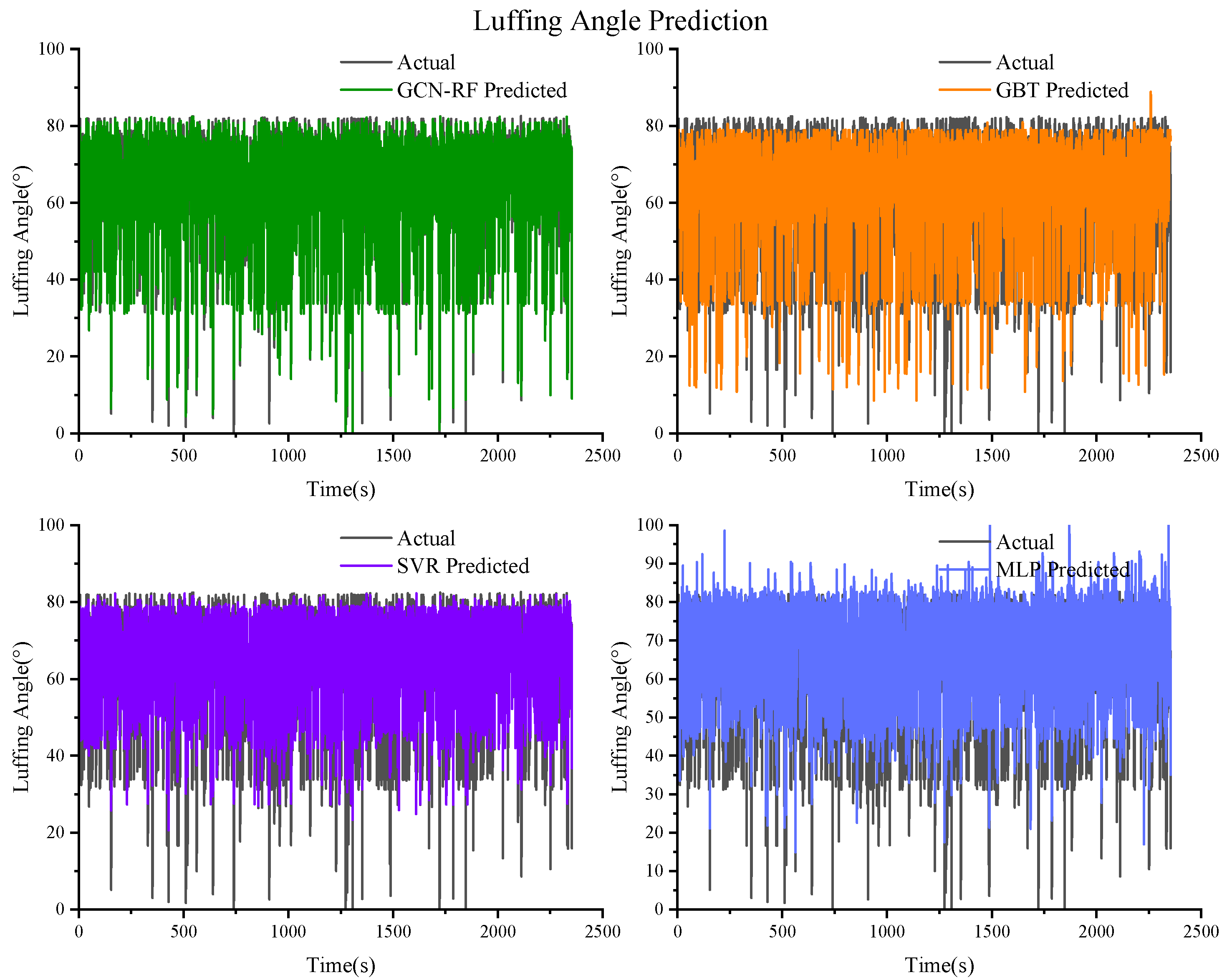
The prediction results of the luffing angle are shown in Figure 23 and the R2, MSE, and RMSE of GCN–RF, GBT, SVR, and MLP are shown in Table 15.
Figure 23 illustrates a comparison between the actual and predicted values of the GCN–RF, GBT, SVR, and MLP in predicting amplitude angle. The results indicate that the prediction curve generated by the GCN–RF nearly coincides with the actual curve, suggesting an exceptionally high level of predictive accuracy. The GBT also demonstrates commendable performance, as its predictions closely follow the actual values, albeit with minor discrepancies in regions characterized by fluctuations. Conversely, the prediction curves for the SVR and MLP exhibit considerable divergence from the actual values, particularly during intervals of rapid data variation.
Table 15 provides the R2, MSE, and RMSE metrics for each model. The GCN–RF achieves an R2 value of 0.9793, which is nearly equal to 1, thereby reflecting its superior explanatory power and fitting capability. The corresponding MSE and RMSE values are 0.0027 and 0.0517, respectively, both of which are the lowest among the models, further substantiating the GCN–RF’s high accuracy in amplitude angle prediction. The GBT presents an R2 value of 0.9660, an MSE of 0.0046, and an RMSE of 0.0678, demonstrating that it retains a robust predictive capacity. The SVR exhibits an R2 value of 0.9283, an MSE of 0.0095, and an RMSE of 0.0974, indicating a moderate performance in the amplitude angle prediction task, characterized by relatively lower accuracy. The MLP records an R2 value of 0.9150, an MSE of 0.0121, and an RMSE of 0.1046. Consequently, both the MLP and SVR exhibit greater prediction errors and demonstrate less stable performance.
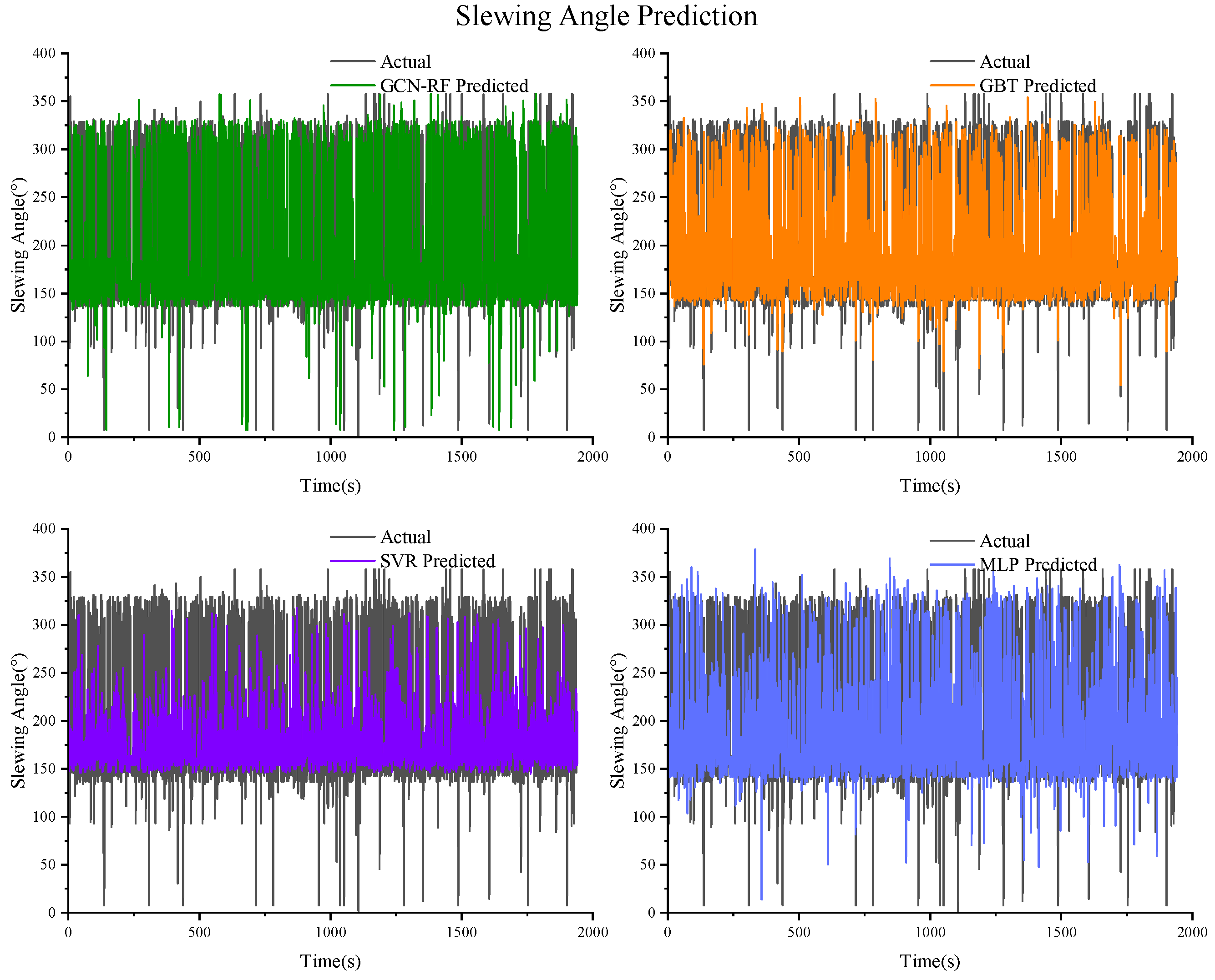
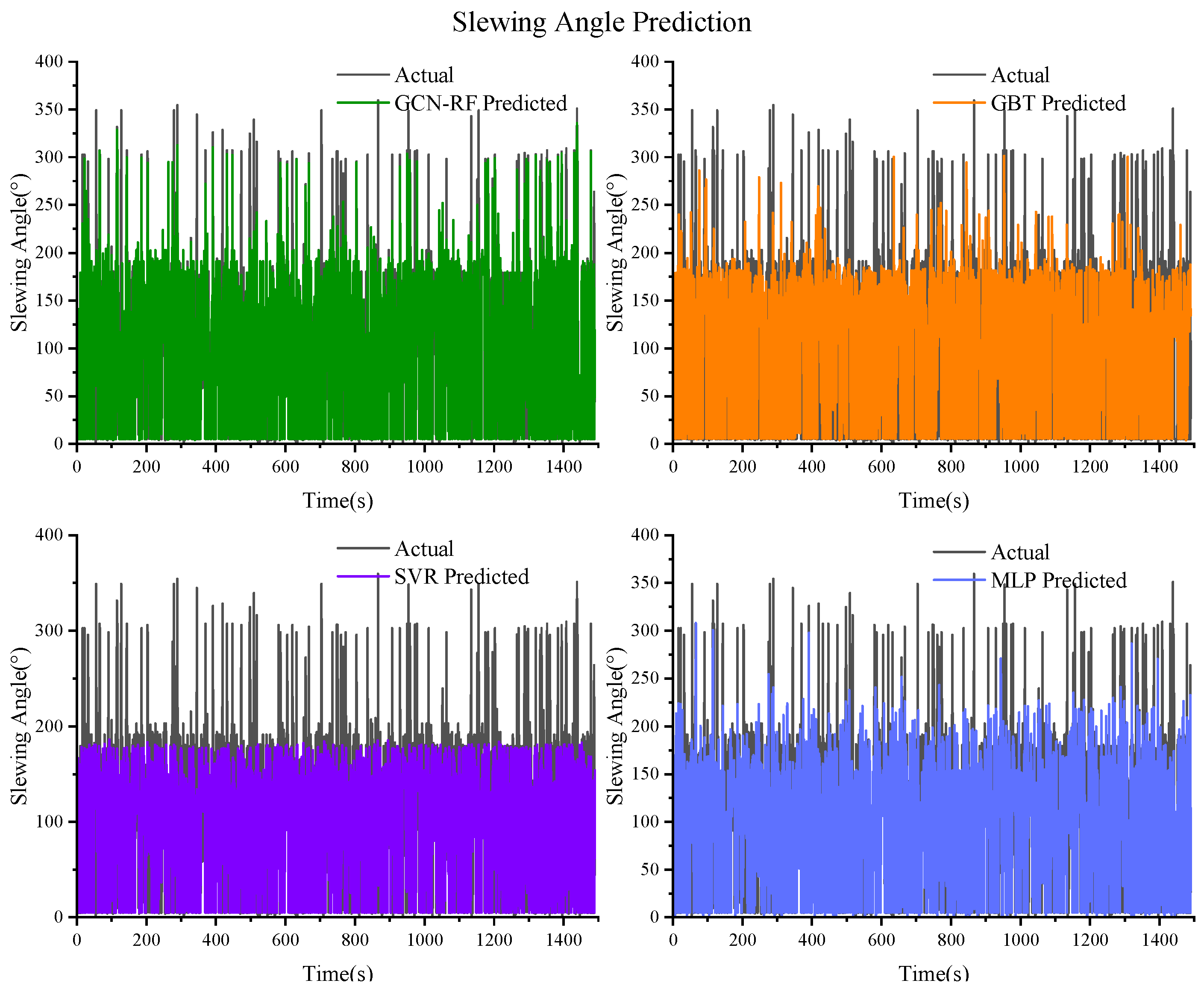
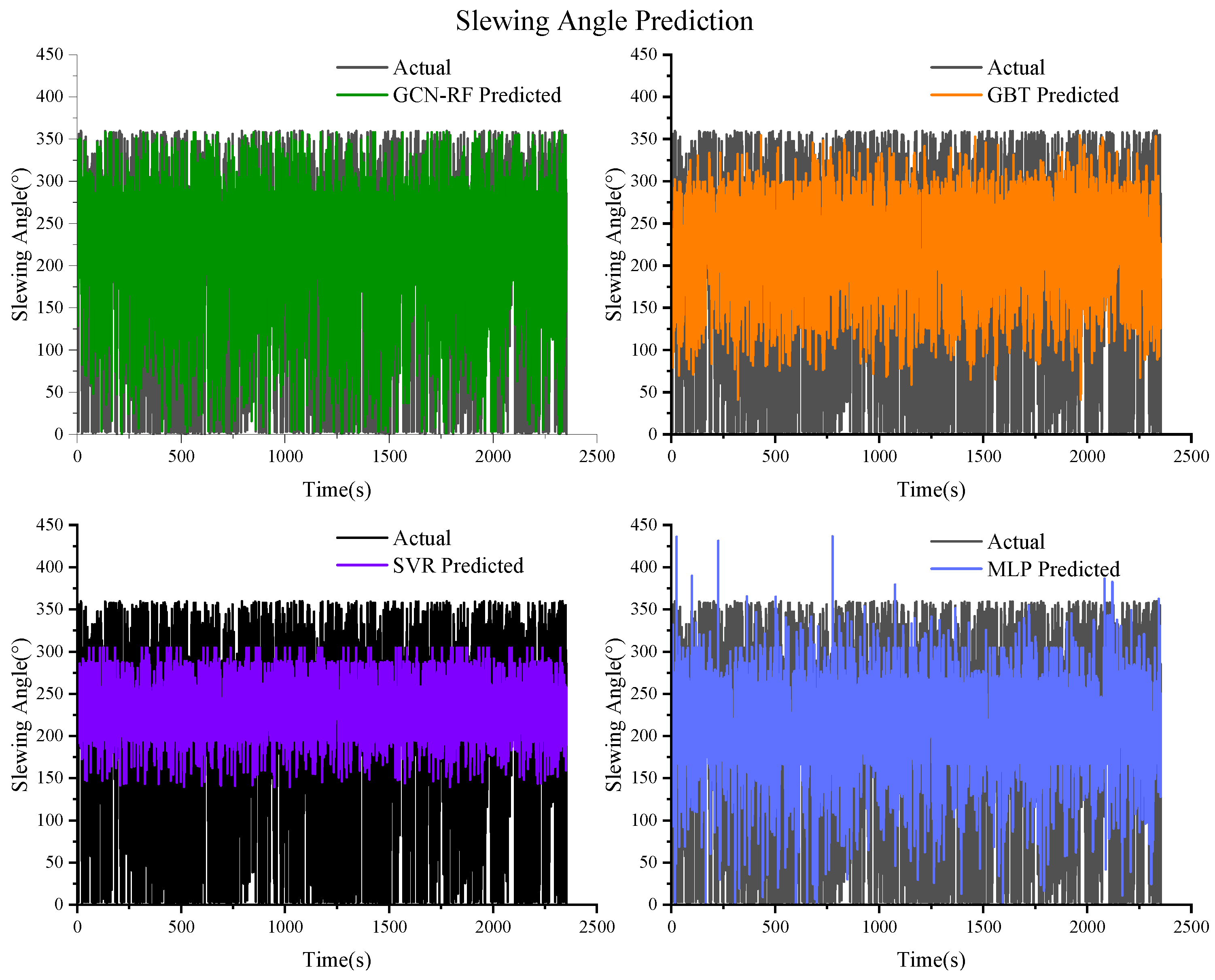
The prediction results of the slewing angle are shown in Figure 24 and the R2, MSE, and RMSE of GCN–RF, GBT, SVR, and MLP are shown in Table 16.
Figure 24 illustrates a comparison between the actual and predicted values of the GCN–RF, GBT, SVR, and MLP in predicting slewing angle. It is evident that while the prediction curve generated by the GCN–RF exhibits a degree of alignment with the actual curve, its accuracy has diminished relative to prior predictions. The GBT also demonstrates significant deviations from the actual values, particularly in regions characterized by substantial data variability. In contrast, the prediction curves for the SVR and MLP reveal even greater discrepancies from the actual values, especially in areas with frequent fluctuations, thereby indicating a diminished performance in the prediction of slewing angle prediction.
Table 16 provides the R2, MSE, and RMSE metrics for each model. The GCN–RF achieves the highest R2 value of 0.8220 among the four models, signifying a relatively strong explanatory capacity in slewing angle prediction, albeit with a notable decline in performance compared to earlier assessments. The MSE and RMSE values for this model are 0.0118 and 0.1084, respectively, reflecting a certain degree of predictive error. The GBT presents an R2 value of 0.7836, with an MSE of 0.0144 and an RMSE of 0.1201, demonstrating that it retains some predictive efficacy for this task. Conversely, the SVR exhibits an R2 value of 0.6738, an MSE of 0.0225, and an RMSE of 0.1501, indicating inadequate performance in slewing angle prediction, characterized by low predictive accuracy. The MLP records the lowest R2 value of 0.6702, alongside an MSE of 0.0244 and an RMSE of 0.1473, reflecting substantial prediction errors and a lack of stability.
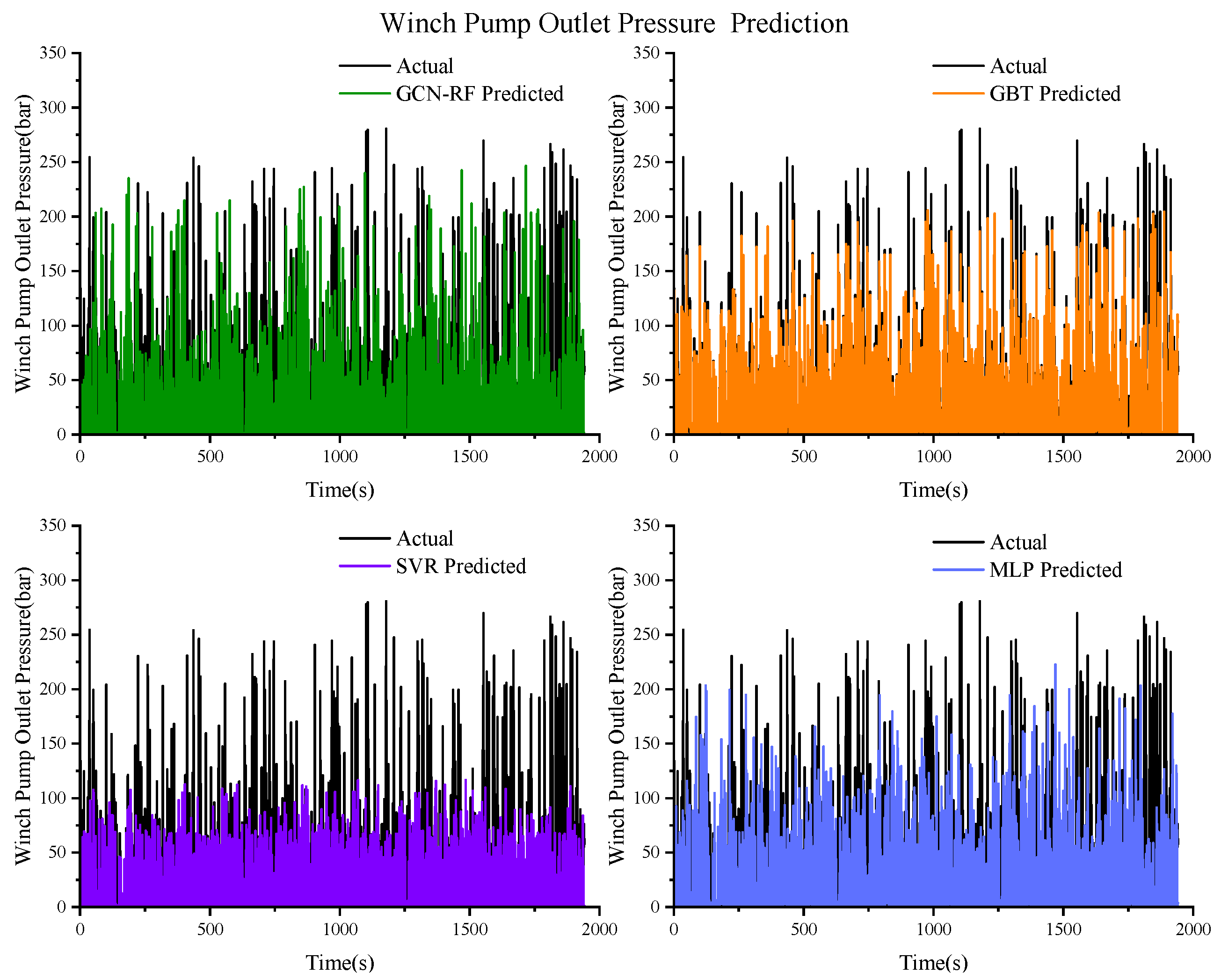
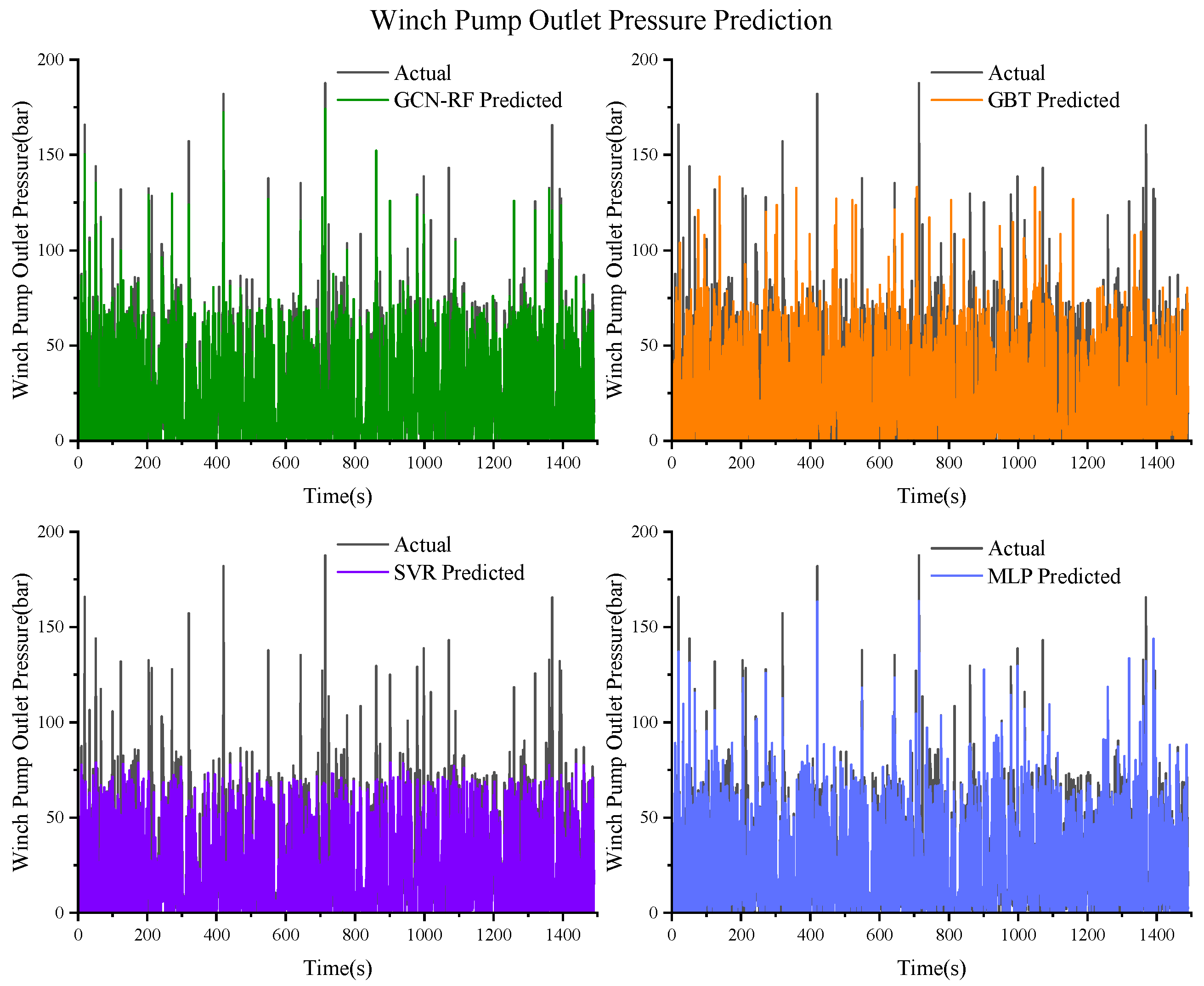
The prediction results of the winch pump outlet pressure are shown in Figure 25 and the R2, MSE, and RMSE of GCN–RF, GBT, SVR, and MLP are shown in Table 17.
Figure 25 illustrates a comparison between the actual and predicted values of the GCN–RF, GBT, SVR, and MLP in predicting winch pump outlet pressure. The data presented in the figure indicate that the prediction trajectories of the GCN–RF and GBT closely align with the actual curve, suggesting a superior level of predictive accuracy. Notably, the GBT consistently yields predictions that are close to the actual values across most scenarios. Conversely, the prediction trajectories of the SVR and MLP demonstrate significant deviations from the actual values, particularly during periods characterized by substantial data fluctuations, indicating that these models exhibit inferior performance relative to the GCN–RF and GBT in the prediction of winch pump outlet pressure.
Table 17 provides the R2, MSE, and RMSE metrics for each model. The GBT achieves the highest R2 value of 0.8999, signifying its optimal performance in terms of explanatory power and fitting capability. The corresponding MSE and RMSE values are 0.0021 and 0.0459, respectively, further substantiating the GBT’s high predictive accuracy in this application. The GCN–RF presents an R2 value of 0.8932, an MSE of 0.0022, and an RMSE of 0.0474, which are slightly lower values than those of the GBT model and still indicate robust predictive capability. In contrast, the SVR exhibits an R2 value of 0.8119, with an MSE of 0.0067 and an RMSE of 0.0687, indicating average performance in the winch pump outlet pressure prediction and relatively diminished predictive accuracy. The MLP records the lowest R2 value of 0.7928, accompanied by an MSE of 0.0074 and an RMSE of 0.0750, reflecting greater prediction errors and a lack of stability in its performance.
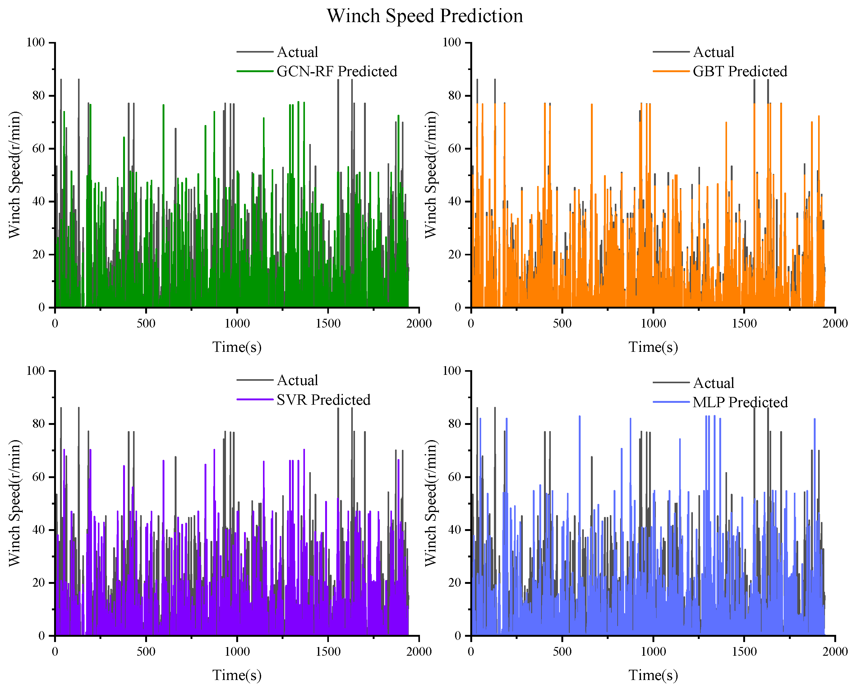
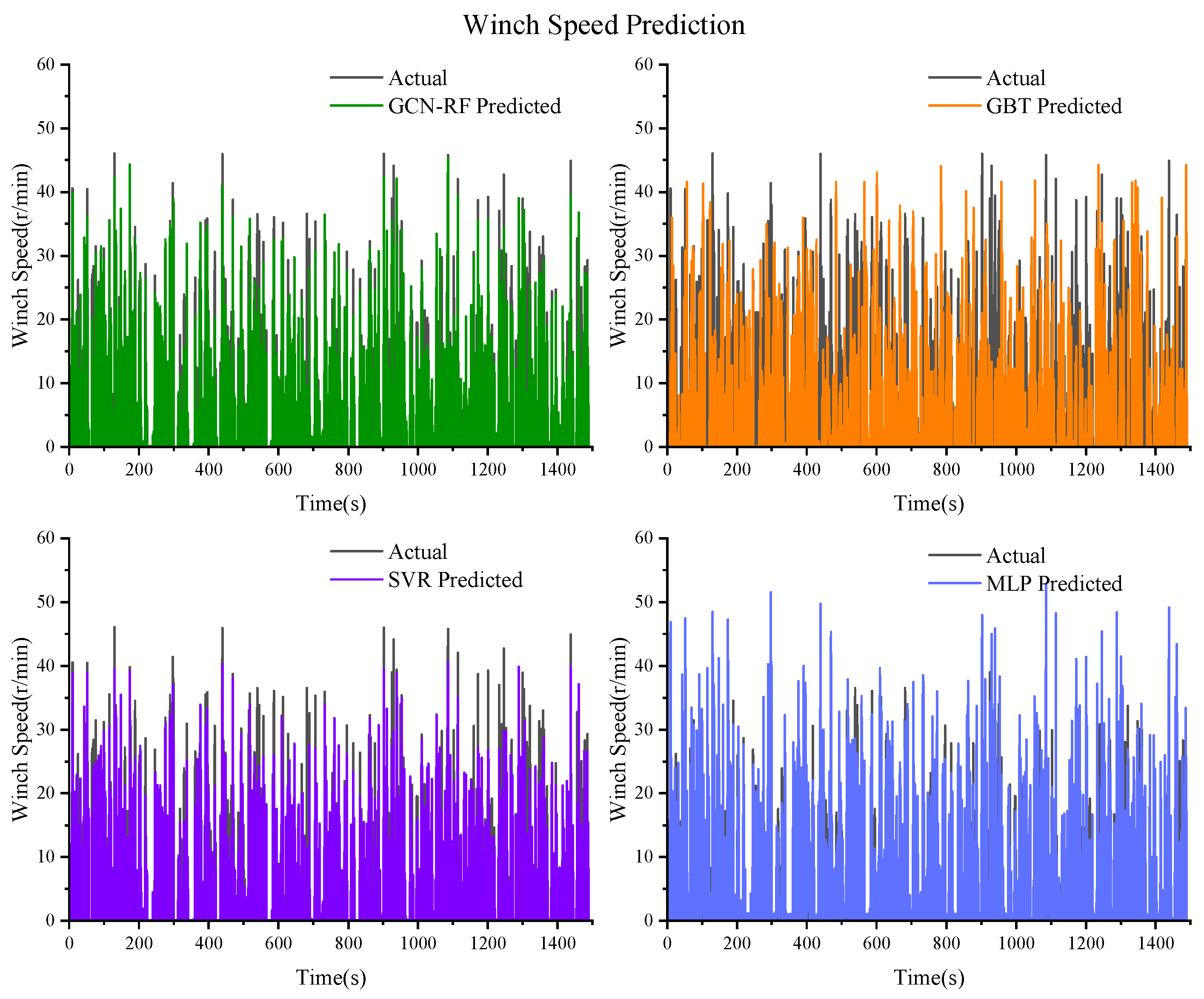
The prediction results of the winch speed are shown in Figure 26 and the R2, MSE, and RMSE of GCN–RF, GBT, SVR, and MLP are shown in Table 18.
Figure 26 illustrates a comparison between the actual and predicted values of the GCN–RF, GBT, SVR, and MLP in predicting winch speed. The prediction trajectories of the GCN–RF and GBT closely align with the actual curve, suggesting a commendable level of predictive accuracy. Notably, the GBT demonstrates a high degree of correlation with the actual values across most instances. Conversely, the prediction trajectories of the SVR and MLP reveal significant deviations from the actual values, particularly in regions characterized by substantial speed fluctuations, indicating that these models do not perform as effectively as the GCN–RF and GBT in the prediction of winch speed.
Table 18 provides the R2, MSE, and RMSE metrics for each model. The GBT achieves the highest R2 value of 0.9058, signifying superior performance in terms of explanatory power and fitting capability. The corresponding MSE and RMSE values are 0.0042 and 0.0630, respectively, further substantiating the GBT’s high predictive accuracy in this context. The GCN–RF presents an R2 value of 0.8866, with an MSE of 0.0049 and an RMSE of 0.0699, demonstrating that it also maintains a commendable level of predictive performance. In contrast, the SVR exhibits an R2 value of 0.8174, an MSE of 0.0083, and an RMSE of 0.0939, indicating average performance in the winch speed prediction task, with relatively lower predictive accuracy. The MLP records an R2 value of 0.8592, an MSE of 0.0061, and an RMSE of 0.0779, reflecting marginally better performance than the SVR. However, it still exhibits considerable prediction errors.

3.5. Key Variables Prediction Results of the 240 t Truck Crane

The prediction results of the amplitude are shown in Figure 27 and the R2, MSE, and RMSE of GCN–RF, GBT, SVR, and MLP are shown in Table 19.
Figure 27 illustrates a comparison between the actual and predicted values of the GCN–RF, GBT, SVR, and MLP in predicting amplitude. The results indicate that the prediction curves for the GCN–RF and GBT closely align with the actual curve, suggesting a high degree of predictive accuracy. Notably, the prediction curve of the GCN–RF nearly coincides with the actual data. Conversely, the prediction curves for the SVR and MLP exhibit considerable divergence from the actual values, particularly in regions characterized by significant data fluctuations, indicating inferior performance in amplitude prediction relative to the GCN–RF and GBT.
Table 19 provides the R2, MSE, and RMSE metrics for each model. The GCN–RF achieves the highest R2 value of 0.9872 among the four models, signifying superior explanatory power and fitting capability. The MSE and RMSE values for this model are 0.0011 and 0.0330, respectively, both of which are the lowest recorded, further substantiating the GCN–RF’s high precision in amplitude prediction. The GBT presents an R2 value of 0.9770, an MSE of 0.0020, and an RMSE of 0.0448, demonstrating commendable predictive performance. In contrast, the SVR exhibits an R2 value of 0.8216, an MSE of 0.1234, and an RMSE of 0.1213, indicating markedly inferior values to those of the GCN–RF and GBT, thereby reflecting lower prediction accuracy. The MLP records an R2 value of 0.9546, an MSE of 0.0039, and an RMSE of 0.0623. While it performs slightly better than the SVR model, it still demonstrates greater prediction errors.
The prediction results of the boom length are shown in Figure 28 and the R2, MSE, and RMSE of GCN–RF, GBT, SVR, and MLP are shown in Table 20.
Figure 28 illustrates a comparative analysis of the actual and predicted values generated by the GCN–RF, GBT, SVR, and MLP in the context of boom length prediction. The prediction curves for the GCN–RF and GBT closely approximate the actual curves, indicating a high level of predictive accuracy. Notably, the GCN–RF’s prediction curve consistently aligns with the actual values across most instances. Conversely, the prediction curves for the SVR and MLP demonstrate considerable divergence from the actual values, particularly in regions characterized by significant data fluctuations, suggesting inferior performance in boom length prediction relative to the GCN–RF and GBT.
Table 20 provides the R2, MSE, and RMSE values for each model. The GCN–RF achieves the highest R2 value of 0.9223 among the four models, signifying superior performance in terms of explanatory power and fitting capability. The MSE and RMSE values for this model are 0.0080 and 0.0893, respectively, both of which are the lowest recorded, further substantiating the GCN–RF’s high precision in boom length prediction. The GBT presents an R2 value of 0.8945, an MSE of 0.0108, and an RMSE of 0.1010, demonstrating commendable predictive performance. In contrast, the SVR exhibits an R2 value of 0.8095, an MSE of 0.0197, and an RMSE of 0.1404, all of which are significantly lower than those of the GCN–RF and GBT, indicating diminished prediction accuracy. The MLP records the lowest R2 value at 0.8573, with an MSE of 0.0144 and an RMSE of 0.1211. While it performs slightly better than the SVR, it still demonstrates greater prediction errors.
The prediction results of the flexible pump pressure are shown in Figure 29 and the R2, MSE, and RMSE of GCN–RF, GBT, SVR, and MLP are shown in Table 21.
Figure 29 illustrates the comparison between the actual and predicted values for the GCN–RF, GBT, SVR, and MLP in predicting flexible pump pressure. It is evident that the prediction curves for the GCN–RF and GBT closely match the actual curves, indicating strong prediction accuracy. Notably, the GCN–RF’s prediction curve aligns well with the actual values in most instances. In contrast, the SVR and MLP show a significant discrepancy from the actual values, particularly in areas with large pressure fluctuations, indicating that these models are less effective in predicting flexible pump pressure compared to GCN–RF and GBT.
Table 21 provides the R2, MSE, and RMSE values for each model. The GCN–RF achieves the highest R2 value of 0.8504 among the four models, signifying superior performance in explanatory power and fitting capability. Its MSE and RMSE values are 0.0054 and 0.0736, respectively, both of which are the lowest, further substantiating the GCN–RF’s high precision in predicting flexible pump pressure. The GBT presents an R2 value of 0.8349, an MSE of 0.0065, and an RMSE of 0.0806, demonstrating strong predictive performance. On the other hand, the SVR exhibits an R2 value of 0.7716, an MSE of 0.0102, and an RMSE of 0.1009, which are significantly lower than those of the GCN–RF and GBT, indicating diminished prediction accuracy. The MLP records an R2 value of 0.7983, an MSE of 0.0076, and an RMSE of 0.0872. While it performs slightly better than SVR, it still exhibits greater prediction errors.
The prediction results of the height are shown in Figure 30 and the R2, MSE, and RMSE of GCN–RF, GBT, SVR, and MLP are shown in Table 22.
Figure 30 illustrates a comparison between the actual and predicted values of the GCN–RF, GBT, SVR, and MLP in predicting height. It is evident that the prediction curve of the GCN–RF closely aligns with the actual curve, suggesting a high level of accuracy. The GBT also performs well, although it shows some discrepancies from the actual values in areas with significant fluctuations. In contrast, the prediction curves for the SVR and MLP exhibit a greater divergence from the actual values, especially in regions with sharp changes in height, indicating that these models are less effective in height prediction compared to GCN–RF and GBT.
Table 22 provides the R2, MSE, and RMSE values for each model. The GCN–RF achieves the highest R2 value of 0.8804 among the four models, signifying its superior performance in explanatory power and fitting ability. Its MSE and RMSE values are 0.0047 and 0.0685, respectively, both of which are the lowest, further substantiating the GCN–RF’s high precision in height prediction. The GBT presents an R2 value of 0.8228, an MSE of 0.0067, and an RMSE of 0.0821, demonstrating good predictive capability as well. The SVR exhibits an R2 value of 0.7097, an MSE of 0.0110, and an RMSE of 0.1054, which are considerably lower than those of the GCN–RF and GBT, indicating diminished prediction accuracy. The MLP records an R2 value of 0.6844, an MSE of 0.0124, and an RMSE of 0.1112, reflecting even greater prediction errors and lower accuracy.
The prediction results of the luffing angle are shown in Figure 31 and the R2, MSE, and RMSE of GCN–RF, GBT, SVR, and MLP are shown in Table 23.
Figure 31 illustrates the comparison between actual and predicted values for the GCN–RF, GBT, SVR, and MLP in predicting the luffing angle. It is evident that the prediction curves for the GCN–RF and GBT models closely align with the actual curves, suggesting a high level of accuracy. Notably, the GCN–RF consistently demonstrates a strong match with the actual values. In contrast, the SVR and MLP exhibit a significant discrepancy from the actual values, particularly in areas with more pronounced angle variations, suggesting that these models are less effective in predicting the luffing angle compared to GCN–RF and GBT.
Table 23 provides the R2, MSE, and RMSE values for each model. The GCN–RF achieves the highest R2 value of 0.9678 among the four models, signifying its superior explanatory power and fitting capability. Its MSE and RMSE values are 0.0011 and 0.0338, respectively, both of which are the lowest, further substantiating the GCN–RF’s high precision in amplitude angle prediction. The GBT presents an R2 value of 0.9261, an MSE of 0.0026, and an RMSE of 0.0511, demonstrating strong predictive performance. The SVR exhibits an R2 value of 0.7484, an MSE of 0.0092, and an RMSE of 0.0962, which are significantly lower than those of the GCN–RF and GBT, indicating diminished prediction accuracy. The MLP records an R2 value of 0.7335, an MSE of 0.0094, and an RMSE of 0.0972, reflecting slightly better performance than SVR but still reflecting greater prediction errors.
The prediction results of the slewing angle are shown in Figure 32 and the R2, MSE, and RMSE of GCN–RF, GBT, SVR, and MLP are shown in Table 24.
Figure 32 illustrates the comparison between the actual and predicted values for the GCN–RF, GBT, SVR, and MLP in predicting slewing angles. The figure reveals a noticeable gap between the prediction curves and the actual curves across all models, indicating that the prediction accuracy for each model is relatively low in this context. Notably, the SVR and MLP show considerable discrepancies from the actual values, particularly in areas with more significant angle variations, highlighting their limited predictive capabilities. On the other hand, the GCN–RF performs comparatively better than the others, although its results still do not meet expectations when compared to other models.
Table 24 provides the R2, MSE, and RMSE values for each model. The GCN–RF achieves the highest R2 value of 0.5705 among the four models, signifying a relatively better ability to explain and fit the data in slewing angle prediction, though it is still not optimal. Its MSE and RMSE values are 0.0480 and 0.2190, respectively, which are the best among the models but still indicate significant error, reflecting limited prediction accuracy. The GBT presents an R2 value of 0.4239, an MSE of 0.0642, and an RMSE of 0.2534, demonstrating average performance. The SVR exhibits an R2 value of 0.3255, an MSE of 0.0752, and an RMSE of 0.2752, indicating lower prediction accuracy. Lastly, the MLP records the lowest R2 value of 0.2514, with an MSE of 0.0724 and an RMSE of 0.2692, reflecting the weakest performance in slewing angle prediction.
The prediction results of the winch pump outlet pressure are shown in Figure 33 and the R2, MSE, and RMSE of GCN–RF, GBT, SVR, and MLP are shown in Table 25.
Figure 33 illustrates the comparison between the actual and predicted values of the GCN–RF, GBT, SVR, and MLP in predicting the winch pump outlet pressure. It is evident that the prediction curves for the GCN–RF and GBT closely match the actual curves, suggesting a high level of prediction accuracy. Notably, the GBT consistently aligns well with the actual values. In contrast, the SVR and MLP exhibit a significant disparity between their prediction curves and the actual values, particularly in areas with more data fluctuations, suggesting that these models are less effective than GCN–RF and GBT in the prediction of the winch pump outlet pressure.
Table 25 provides the R2, MSE, and RMSE values for each model. The GBT achieves the highest R2 value of 0.9195 among the four models, signifying its superior explanatory power and fitting capability. Its MSE and RMSE values are 0.0018 and 0.0430, respectively, which are the lowest, further substantiating the GBT’s high precision in predicting winch pump outlet pressure. The GCN–RF presents an R2 value of 0.9167, an MSE of 0.0020, and an RMSE of 0.0452, demonstrating strong predictive ability. However, the SVR exhibits an R2 value of 0.3736, an MSE of 0.0065, and an RMSE of 0.0804, indicating significantly poorer performance compared to GCN–RF and GBT, with lower prediction accuracy. The MLP records an R2 value of 0.8889, an MSE of 0.0028, and an RMSE of 0.0525. While it performs better than SVR, it still does not measure up to GCN–RF and GBT.
The prediction results of the winch speed are shown in Figure 34 and the R2, MSE, and RMSE of GCN–RF, GBT, SVR, and MLP are shown in Table 26.
Figure 34 illustrates the comparison between the actual and predicted values for the GCN–RF, GBT, SVR, and MLP in predicting the winch speed. It is evident that the prediction curve of the GBT model closely aligns with the actual curve, suggesting a high level of accuracy. The GCN–RF also shows strong consistency with the actual values, following closely behind. In contrast, the SVR and MLP display a greater gap between their prediction curves and the actual values, especially in areas with significant speed variations, indicating that these models are less effective than GBT and GCN–RF in predicting the winch speed.
Table 26 provides the R2, MSE, and RMSE values for each model. The GBT achieves the highest R2 value of 0.9088 among the four models, signifying the best explanatory power and fitting capability. Its MSE and RMSE values are 0.0030 and 0.0552, respectively, which are the lowest, further substantiating the GBT’s high precision in winch speed prediction. The GCN–RF ranks second with an R2 value of 0.8690, an MSE of 0.0040, and an RMSE of 0.0631, indicating good predictive performance. The SVR exhibits an R2 value of 0.8466, an MSE of 0.0057, and an RMSE of 0.0707, indicating significantly poorer performance compared to GCN–RF and GBT, with lower prediction accuracy. The MLP records an R2 value of 0.8701, an MSE of 0.0043, and an RMSE of 0.0657. While it performs better than SVR, it still does not match the effectiveness of GBT and GCN–RF.

4. Discussion and Results

This research confirms the effectiveness of the GCN–RF model by utilizing datasets from the operational conditions of three cranes with capacities of 160 t, 200 t, and 240 t, as detailed below.
(1)
For the 160 t crane, the prediction analysis of eight target variables reveals that the GCN–RF model achieves the highest accuracy for seven of them: amplitude, boom length, flexible pump pressure, luffing angle, slewing angle, winch pump outlet pressure, and winch speed. In terms of height, the GCN–RF model’s accuracy is slightly lower than that of GBT, with scores of 0.9248 and 0.9260, respectively, both demonstrating strong predictive performance. Overall, the GCN–RF model shows reliable predictive capabilities across all eight target variables.
(2)
For the 200 t crane, the analysis indicates that the GCN–RF model achieves the highest accuracy for six target variables: amplitude, boom length, flexible pump pressure, height, luffing angle, and slewing angle. For winch pump outlet pressure and winch speed, the GCN–RF model records accuracies of 0.8932 and 0.8866, while GBT scores 0.8999 and 0.9088, respectively, both still reflecting high prediction performance. A thorough analysis confirms that the GCN–RF model performs well for all eight target variables.
(3)
For the 240 t crane, the prediction analysis shows that the performance for the slewing angle is relatively low. Nevertheless, the GCN–RF model achieves the highest accuracy for five target variables: amplitude, boom length, flexible pump pressure, height, and luffing angle. For winch pump outlet pressure and winch speed, the GCN–RF model’s accuracies are 0.9167 and 0.8690, while GBT achieves 0.9195 and 0.8908, both maintaining strong prediction performance. Overall, the GCN–RF model demonstrates good predictive performance for seven target variables except slewing angle.
In summary, as the lifting capacity of the crane increases, the prediction performance of the GCN–RF model for the target variables varies. From the data of the 160 t, 200 t, and 240 t cranes, the GCN–RF model achieves the highest accuracy for seven, six, and five target variables, respectively. However, it consistently shows good predictive performance for nearly all target variables. Future research will focus on improving the accuracy of the target variables that showed lower performance.

5. Conclusions

This paper proposes a multi-input and multi-output soft sensing model based on GCN–RF to obtain the key performance indicators of the four operating systems of truck cranes: slewing, luffing, telescoping, and winching. These indicators primarily include amplitude, boom length, flexible pump pressure, height, luffing angle, slewing angle, winch pump outlet pressure, and winch speed. The difficulty in obtaining key indicators is due to the complexity, time-varying, and coupling of operating conditions. Based on the real operation data verification results of 160 t, 200 t, and 240 t truck cranes and the comparison with GBT, SVR, and MLP, the following conclusions can be made.
(1) For the 160 t crane data, the GCN–RF outperformed GBT, SVR, and MLP in prediction accuracy across all seven metrics, except for height, where GBT achieved the highest accuracy of 0.926, while GCN–RF had an accuracy of 0.9248. This suggests that GCN–RF has strong predictive capabilities for almost all target variables.
(2) For the 200 t crane data, GCN–RF’s prediction accuracy for winch pump outlet pressure and winch speed was slightly lower than that of GBT. However, it outperformed GBT, SVR, and MLP in accuracy for the other six metrics, indicating that GCN–RF continues to perform well for nearly all target variables.
(3) For the 240 t crane data, all four models showed relatively low prediction accuracy for slewing angle. GCN–RF’s accuracy for winch pump outlet pressure and winch speed was still below that of GBT. Nonetheless, GCN–RF achieved higher accuracy than GBT, SVR, and MLP for the other five metrics, demonstrating that it maintains good predictive performance for almost all target variables, except for slewing angle.
While GCN–RF has demonstrated promising performance in predicting truck crane operational performance indicators, there are still certain issues that require additional research. Further investigation is required to assess the robustness and generalization capabilities of GCN–RF. Moreover, prospective research avenues should encompass performance evaluation, anomaly detection, and fault diagnosis for cranes utilizing the predicted data.

Author Contributions

Conceptualization, S.J. and W.J.; methodology, S.J., B.Z. and W.L.; software, S.J. and W.J.; validation, S.J. and B.Z.; formal analysis, S.J. and W.J.; investigation, S.J. and B.Z.; resources, Y.W., B.Z. and W.L.; data curation, S.J. and W.L.; writing—original draft preparation, S.J., B.Z. and W.J.; writing—review and editing, S.J., B.Z. and S.-K.N.; funding acquisition, B.Z. All authors have read and agreed to the published version of the manuscript.

Funding

This research was funded by the Fundamental Research Funds for the Central Universities, grant number 2019ZDPY08.

Data Availability Statement

The sulfur recovery and the debutanizer column datasets can be obtained from https://github.com/softsensors/MIMOdata (accessed on 10 September 2024).

Acknowledgments

The authors would like to acknowledge the support of Xuzhou Heavy Machinery Co., Ltd. of the experiment in Xuzhou, China.

Conflicts of Interest

The authors declare no conflicts of interest.

References

  1. Xie, H.B.; Zhang, G.L. Research on Characteristics of the Piloted Follow-up Load Control Valve in Automobile Crane Luffing System. In Proceedings of the 2013 Fifth International Conference on Measuring Technology and Mechatronics Automation, Hong Kong, China, 16–17 January 2013; pp. 887–892. [Google Scholar]
  2. Ali, G.M.; Mansoor, A.; Liu, S.; Olearczyk, J.; Bouferguene, A. Decision support for hydraulic crane stabilization using combined loading and crane mat strength analysis. Automat. Constr. 2021, 131, 103884. [Google Scholar] [CrossRef]
  3. Sadeghi, S.; Soltanmohammadlou, N.; Rahnamayiezekavat, P. A systematic review of scholarly works addressing crane safety requirements. Saf. Sci. 2021, 133, 105002. [Google Scholar] [CrossRef]
  4. Huang, J.; Ma, H.X.; Wei, Q. Research on the Fretting Performance of Truck Crane Hoist System Based on AMESim. In Proceedings of the 2017 4th International Conference on Information Science and Control Engineering (ICISCE), Changsha, China, 21–23 July 2017; pp. 1187–1192. [Google Scholar]
  5. Moi, T.; Cibicik, A.; Rølvåg, T. Digital twin-based condition monitoring of a knuckle boom crane: An experimental study. Eng. Fail. Anal. 2020, 112, 104517. [Google Scholar] [CrossRef]
  6. Cekus, D.; Kwiatoń, P. Effect of the rope system deformation on the working cycle of the mobile crane during interaction of wind pressure. Mech. Mach. Theory 2020, 153, 104011. [Google Scholar] [CrossRef]
  7. Price, L.C.; Chen, J.D.; Park, J.; Cho, Y.K. Multisensor-driven real-time crane monitoring system for blind lift operations: Lessons learned from a case study. Automat. Constr. 2021, 124, 103552. [Google Scholar] [CrossRef]
  8. Du, W.L.; Han, S.G.; Song, X.W.; Tian, S.X.; Pecht, M. Condition Monitoring Model of a Hydraulic System in Truck Crane. In Proceedings of the 2018 IEEE International Conference on Prognostics and Health Management (ICPHM), Seattle, WA, USA, 11–13 June 2018; pp. 1–5. [Google Scholar]
  9. Zhou, C.; Luo, H.B.; Fang, W.L.; Wei, R.; Ding, L.Y. Cyber-physical-system-based safety monitoring for blind hoisting with the internet of things: A case study. Automat. Constr. 2019, 97, 138–150. [Google Scholar] [CrossRef]
  10. Jiang, W.G.; Liu, Y.H.; Chen, K.; Liu, Y.H. Early-warning of unsafe hoisting operations: An integration of digital twin and knowledge graph. Dev. Built Environ. 2024, 19, 100490. [Google Scholar] [CrossRef]
  11. Mukherjee, A.; Sasidharan, M.; Herrera, M.; Parlikad, A.K. Unsupervised constrained discord detection in IoT-based online crane monitoring. Adv. Eng. Inform. 2024, 60, 102444. [Google Scholar] [CrossRef]
  12. Kargar, V.; Jahangiri, M.; Alimohammadlu, M.; Kamalinia, M.; Mirazahossieninejad, M. Risk assessment of mobile crane overturning in Asymmetric Tandem Lifting (ATL) operation based on fuzzy fault tree analysis (FFTA). Results Eng. 2022, 16, 100755. [Google Scholar] [CrossRef]
  13. Hussain, M.; Ye, Z.; Chi, H.L.; Hsu, S.C. Predicting degraded lifting capacity of aging tower cranes: A digital twin-driven approach. Adv. Eng. Inform. 2024, 59, 102310. [Google Scholar] [CrossRef]
  14. Huang, H.Z. Reliability evaluation of a hydraulic truck crane using field data with fuzziness. Microelectron. Reliab. 1996, 36, 1531–1536. [Google Scholar] [CrossRef]
  15. Ramli, L.; Mohamed, Z.; Abdullahi, A.M.; Jaafar, H.I.; Lazim, I.M. Control strategies for crane systems: A comprehensive review. Mech. Syst. Signal Process. 2017, 95, 1–23. [Google Scholar] [CrossRef]
  16. An, J.Q.; Wu, M.; She, J.H.; Terano, T. Re-optimization strategy for truck crane lift-path planning. Automat. Constr. 2018, 90, 146–155. [Google Scholar] [CrossRef]
  17. Hu, S.B.; Fang, Y.H.; Bai, Y. Automation and optimization in crane lift planning: A critical review. Adv. Eng. Inform. 2021, 49, 101346. [Google Scholar] [CrossRef]
  18. Cai, P.P.; Cai, Y.Y.; Chandrasekaran, I.; Zheng, J.M. Parallel genetic algorithm based automatic path planning for crane lifting in complex environments. Automat. Constr. 2016, 62, 133–147. [Google Scholar] [CrossRef]
  19. Wang, X.; Liu, H. A knowledge-and data-driven soft sensor based on deep learning for predicting the deformation of an air preheater rotor. IEEE Access 2019, 7, 159651–159660. [Google Scholar] [CrossRef]
  20. Gravina, M.; García-Pedrero, A.; Gonzalo-Martín, C.; Sansone, C.; Soda, P. Multi input–Multi output 3D CNN for dementia severity assessment with incomplete multimodal data. Artif. Intell. Med. 2024, 149, 102774. [Google Scholar] [CrossRef] [PubMed]
  21. Zhou, P.W.; Xu, Z.H.; Peng, X.D.; Zhao, J.; Shao, Z.J. Long-term prediction enhancement based on multi-output Gaussian process regression integrated with production plans for oxygen supply network. Comput. Chem. Eng. 2022, 163, 107844. [Google Scholar] [CrossRef]
  22. Jiang, P.; Nie, Y.; Wang, J.Z.; Huang, X.J. Multivariable short-term electricity price forecasting using artificial intelligence and multi-input multi-output scheme. Energy Econ. 2023, 117, 106471. [Google Scholar] [CrossRef]
  23. Qu, Z.K.; Zhang, Y.; Hong, C.; Zhang, C.D.; Dai, Z.W.; Zhao, Y.Y.; Wu, X.D.; Gao, Y.; Jiang, X.M.; Qian, J.; et al. Temperature forecasting of grain in storage: A multi-output and spatiotemporal approach based on deep learning. Comput. Electron. Agric. 2023, 208, 107785. [Google Scholar] [CrossRef]
  24. Li, D.; Yang, C.H.; Li, Y.G.; Zhou, C.; Hunag, D.P.; Liu, Y.Q. A deep semi-supervised learning framework towards multi-output soft sensors development and applications in wastewater treatment processes. J. Water Process Eng. 2024, 57, 104654. [Google Scholar] [CrossRef]
  25. Samal, K.K.R.; Panda, A.K.; Babu, K.S.; Das, S.K. Multi-output TCN autoencoder for long-term pollution forecasting for multiple sites. Urban Clim. 2021, 39, 100943. [Google Scholar] [CrossRef]
  26. Liu, T.; Chen, S.; Yang, P.; Zhu, Y.P.; Harris, C.J. Efficient adaptive deep gradient RBF network for multi-output nonlinear and nonstationary industrial processes. J. Process Control 2023, 126, 1–11. [Google Scholar] [CrossRef]
  27. Rakholia, R.; Le, Q.; Ho, B.Q.; Vu, K.; Carbajo, R.S. Multi-output machine learning model for regional air pollution forecasting in Ho Chi Minh City, Vietnam. Environ. Int. 2023, 173, 107848. [Google Scholar] [CrossRef] [PubMed]
  28. Wang, Y.F.; Xu, L.; Li, J.N.; Ren, Z.Y.; Liu, W.; Ai, Y.H.; Zhou, Y.T.; Li, Q.N.; Zhang, B.Y.; Guo, N.; et al. Multi-output neural network model for predicting biochar yield and composition. Sci. Total Environ. 2024, 945, 173942. [Google Scholar] [CrossRef] [PubMed]
  29. Li, L.H.; Li, N.Q.; Wang, X.; Zhao, J.R.; Zhang, H.S.; Jiao, T.C. Multi-output soft sensor modeling approach for penicillin fermentation process based on features of big data. Expert Syst. Appl. 2023, 213, 119208. [Google Scholar] [CrossRef]
  30. Jia, Z.Y.; Lin, Y.F.; Wang, J.; Zhou, R.H.; Ning, X.J.; He, Y.L.; Zhao, Y.S. GraphSleepNet: Adaptive Spatial-Temporal Graph Convolutional Networks for Sleep Stage Classification. In Proceedings of the Twenty-Ninth International Joint Conference on Artificial Intelligence (IJCAI-20), Yokohama, Japan, 7–15 January 2021; pp. 1324–1330.
  31. Zhou, Y.J.; Jiang, J.; Qian, K.; Ding, Y.L.; Yang, S.H.; He, L.G. Graph convolutional networks-based contamination source identification across water distribution networks. Process Saf. Environ. 2021, 155, 317–324. [Google Scholar] [CrossRef]
  32. Wu, M.; Pan, S.R.; Zhou, C.; Chang, X.J.; Zhu, X.Q. Unsupervised Domain Adaptive Graph Convolutional Networks. In Proceedings of the Web Conference 2020, Taipei Taiwan, 20–24 April 2020; pp. 1457–1467. [Google Scholar]
  33. Wang, G.T.; Zhang, Z.R.; Bian, Z.P.; Xu, Z. A short-term voltage stability online prediction method based on graph convolutional networks and long short-term memory networks. Int. J. Electr. Power Energy Syst. 2021, 127, 106647. [Google Scholar] [CrossRef]
  34. Wan, Y.; Liu, D.; Ren, J.C. A modeling method of wide random forest multi-output soft sensor with attention mechanism for quality prediction of complex industrial processes. Adv. Eng. Inform. 2024, 59, 102255. [Google Scholar] [CrossRef]
  35. Ouyang, H.; Wang, H.Y.; Liu, J.; Zhou, H.B.; Duan, S.Y.; Han, X. Non-probabilistic sensitivity analysis method for multi-input-multi-output structures considering correlations. Int. J. Mech. Sci. 2024, 271, 109123. [Google Scholar] [CrossRef]
  36. Nakano, F.K.; Pliakos, K.; Vens, C. Deep tree-ensembles for multi-output prediction. Pattern Recognit. 2022, 121, 108211. [Google Scholar] [CrossRef]
  37. Qin, Y.; Wei, Z.L.; Chu, D.D.; Zhang, J.C.; Du, Y.F.; Che, Z.M. Artificial neural network-based multi-input multi-output model for short-term storm surge prediction on the southeast coast of China. Ocean Eng. 2024, 300, 116915. [Google Scholar] [CrossRef]
  38. Zhan, X.B.; Zhang, S.C.; Szeto, W.Y. Multi-step-ahead traffic speed forecasting using multi-output gradient boosting regression tree. J. Intell. Transp. Syst. 2020, 24, 125–141. [Google Scholar] [CrossRef]
  39. Tran, N.K.; Kühle, L.C.; Klau, G.W. A critical review of multi-output support vector regression. Pattern Recogn. Lett. 2023, 178, 69–75. [Google Scholar] [CrossRef]
  40. Wang, Z.; Zhou, H.; Zhong, P. Cross-view multi-layer perceptron for incomplete multi-view learning. Appl. Soft Comput. 2024, 157, 111510. [Google Scholar] [CrossRef]
  41. Ji, S.F.; Li, W.; Wang, Y.; Zhang, B.; Ng, S.-K. A Soft Sensor Model for Predicting the Flow of a Hydraulic Pump Based on Graph Convolutional Network–Long Short-Term Memory. Actuators 2024, 13, 38. [Google Scholar] [CrossRef]
Figure 1. The network diagram of GCN with graph data, convolutional layers, and output features.
Actuators 13 00357 g001
Figure 2. RF network architecture diagram with random sampling, decision tree construction, results aggregation, and final prediction.
Actuators 13 00357 g002
Figure 3. GCN–RF architecture diagram with graph data feature extraction and regression prediction.
Actuators 13 00357 g003
Figure 4. Schematic diagram of the truck crane working systems: luffing, slewing, telescoping, and winching systems.
Actuators 13 00357 g004
Figure 5. Schematic diagram of the slewing hydraulic system ((1) oil tank; (2) pump; (3) variable mechanism; (4,5) slewing balance valve; (6) overflow valve; (7) free sliding valve; (8,9) slewing motor; (10,11) brake; (12) pilot pump; (13) filter; (14) reversing valve; (15) slewing brake control valve; (16) accumulator).
Actuators 13 00357 g005
Figure 6. Schematic diagram of the telescopic hydraulic system ((1) 21 filter; (2) oil tank; (3) check valve; (4,5) pump; (6–10) cartridge valve; (11,17,18) two-position four-way solenoid valve; (12,13,16) overflow valve; (14,15) two-position two-way solenoid valve; (19) cylinder arm pin control valve; (20) accumulator; (22) pilot pump; (23,28) arm pin; (24,26) right cylinder pin; (25,27) left cylinder pin; (29) cylinder arm pin solenoid valve; (30) balance valve).
Actuators 13 00357 g006
Figure 7. Schematic diagram of the winch hydraulic system ((1) oil tank; (2) pump; (3) variable mechanism; (4) reversing valve; (5,6) winch balance valve; (7) overflow valve; (8) filter; (9) pilot pump; (10) brake control valve; (11) brake; (12) lifting motor; (13) check valve).
Actuators 13 00357 g007
Figure 8. Schematic diagram of the luffing hydraulic system ((1) 16 filter; (2) oil tank; (3) check valve; (4,5) pump; (6–8) cartridge valve; (9,17) overflow valve; (10) two-position two-way solenoid valve, (11) two-position four-way solenoid valve; (12,13) luffing oil cylinder; (14,15) luffing balance valve; (18) pilot pump).
Actuators 13 00357 g008
Figure 9. Schematic diagram of data acquisition.
Actuators 13 00357 g009
Figure 10. The correlation between target variables and input variables based on GCN.
Actuators 13 00357 g010
Figure 11. Prediction results of the amplitude based on GCN–RF, GBT, SVR, and MLP.
Actuators 13 00357 g011
Figure 12. Prediction results of the boom length based on GCN–RF, GBT, SVR, and MLP.
Actuators 13 00357 g012
Figure 13. Prediction results of the flexible pump pressure based on GCN–RF, GBT, SVR, and MLP.
Actuators 13 00357 g013
Figure 14. Prediction results of the height based on GCN–RF, GBT, SVR, and MLP.
Actuators 13 00357 g014
Figure 15. Prediction results of the luffing angle based on GCN–RF, GBT, SVR, and MLP.
Actuators 13 00357 g015
Figure 16. Prediction results of the slewing angle based on GCN–RF, GBT, SVR, and MLP.
Actuators 13 00357 g016
Figure 17. Prediction results of the winch pump outlet pressure based on GCN–RF, GBT, SVR, and MLP.
Actuators 13 00357 g017
Figure 18. Prediction results of the winch speed based on GCN–RF, GBT, SVR, and MLP.
Actuators 13 00357 g018
Figure 19. Prediction results of the amplitude based on GCN–RF, GBT, SVR, and MLP.
Actuators 13 00357 g019
Figure 20. Prediction results of the boom length based on GCN–RF, GBT, SVR, and MLP.
Actuators 13 00357 g020
Figure 21. Prediction results of the flexible pump pressure based on GCN–RF, GBT, SVR, and MLP.
Actuators 13 00357 g021
Figure 22. Prediction results of the height based on GCN–RF, GBT, SVR, and MLP.
Actuators 13 00357 g022
Figure 23. Prediction results of the luffing angle based on GCN–RF, GBT, SVR, and MLP.
Actuators 13 00357 g023
Figure 24. Prediction results of the slewing angle based on GCN–RF, GBT, SVR, and MLP.
Actuators 13 00357 g024
Figure 25. Prediction results of the winch pump outlet pressure based on GCN–RF, GBT, SVR, and MLP.
Actuators 13 00357 g025
Figure 26. Prediction results of the winch speed based on GCN–RF, GBT, SVR, and MLP.
Actuators 13 00357 g026
Figure 27. Prediction results of the amplitude based on GCN–RF, GBT, SVR, and MLP.
Actuators 13 00357 g027
Figure 28. Prediction results of the boom length based on GCN–RF, GBT, SVR, and MLP.
Actuators 13 00357 g028
Figure 29. Prediction results of the flexible pump pressure based on GCN–RF, GBT, SVR, and MLP.
Actuators 13 00357 g029
Figure 30. Prediction results of the height based on GCN–RF, GBT, SVR, and MLP.
Actuators 13 00357 g030
Figure 31. Prediction results of the luffing angle based on GCN–RF, GBT, SVR, and MLP.
Actuators 13 00357 g031
Figure 32. Prediction results of the slewing angle based on GCN–RF, GBT, SVR, and MLP.
Actuators 13 00357 g032
Figure 33. Prediction results of the winch pump outlet pressure based on GCN–RF, GBT, SVR, and MLP.
Actuators 13 00357 g033
Figure 34. Prediction results of the winch speed based on GCN–RF, GBT, SVR, and MLP.
Actuators 13 00357 g034
Table 1. Variables collected by crane operation system.
Input
Variables
DescriptionOutput
Variables
Description
x1Rated weighty1Amplitude
x2Actual weighty2Boom length
x3Multipliery3Flexible pump pressure
x4Throttle positiony4Height
x5Engine speedy5Luffing angle
x6Luffing handle signaly6Slewing angle
x7Winching handle signaly7Winch pump outlet pressure
x8Slewing handle signaly8Winch speed
x9Telescoping handle signal//
x10Left slewing current//
x11Right slewing current//
x12Flexible pump control current//
x13Luffing balance valve control current//
x14Winch up pump control current//
x15Winch down pump control current//
x16Winch motor control current//
Table 2. GCN–RF model parameter settings.
ModelsNameMain Parameters
GCNNumber of graph convolution layers3
Number of nodes per layer64,128,256
Learning rate0.001
Batch size32
Epoch100
RFNumber of decision trees200
Maximum tree depth30
Minimum number of sample splits2
Minimum number of leaf nodes1
Sample sampling strategyBootstrap
Table 3. R2, MSE, and RMSE values of GCN–RF, GBT, SVR, and MLP.
Target VariablesIndicatorsGCN–RFGBTSVRMLP
AmplitudeR20.88750.86800.61160.6329
MSE0.00310.00360.01080.0101
RMSE0.05560.06030.10390.1007
Table 4. R2, MSE, and RMSE values of GCN–RF, GBT, SVR, and MLP.
Target VariablesIndicatorsGCN–RFGBTSVRMLP
Boom lengthR20.89460.89040.63720.5700
MSE0.00140.00140.00820.0059
RMSE0.03800.03790.09060.0768
Table 5. R2, MSE, and RMSE values of GCN–RF, GBT, SVR, and MLP.
Target VariablesIndicatorsGCN–RFGBTSVRMLP
Flexible pump pressureR20.86890.81240.67670.7200
MSE0.00480.00800.01370.0102
RMSE0.06910.08970.11720.1010
Table 6. R2, MSE, and RMSE values of GCN–RF, GBT, SVR, and MLP.
Target VariablesIndicatorsGCN–RFGBTSVRMLP
HeightR20.92480.92600.80780.8312
MSE0.00150.00140.00470.0034
RMSE0.03880.03740.06890.0583
Table 7. R2, MSE, and RMSE values of GCN–RF, GBT, SVR, and MLP.
Target VariablesIndicatorsGCN–RFGBTSVRMLP
Luffing angleR20.89520.89170.65770.6718
MSE0.00150.00150.00590.0046
RMSE0.03810.03810.07680.0677
Table 8. R2, MSE, and RMSE values of GCN–RF, GBT, SVR, and MLP.
Target VariablesIndicatorsGCN–RFGBTSVRMLP
Slewing angleR20.87520.79750.54630.5220
MSE0.00530.00890.01930.0203
RMSE0.07280.09440.13900.1423
Table 9. R2, MSE, and RMSE values of GCN–RF, GBT, SVR, and MLP.
Target VariablesIndicatorsGCN–RFGBTSVRMLP
Winch pump outlet pressureR20.89480.80890.69170.7216
MSE0.00310.00680.01140.0081
RMSE0.05550.08260.10700.0900
Table 10. R2, MSE, and RMSE values of GCN–RF, GBT, SVR, and MLP.
Target VariablesIndicatorsGCN–RFGBTSVRMLP
Winch speedR20.94620.94230.87400.9177
MSE0.00100.00120.00310.0016
RMSE0.03230.03510.05530.0400
Table 11. R2, MSE, and RMSE values of GCN–RF, GBT, SVR, and MLP.
Target VariablesIndicatorsGCN–RFGBTSVRMLP
AmplitudeR20.92580.91100.77870.8415
MSE0.00230.00290.00780.0050
RMSE0.04830.05420.08840.0706
Table 12. R2, MSE, and RMSE values of GCN–RF, GBT, SVR, and MLP.
Target VariablesIndicatorsGCN–RFGBTSVRMLP
Boom lengthR20.92630.90510.81900.8307
MSE0.00320.00420.01020.0074
RMSE0.05650.06460.10100.0860
Table 13. R2, MSE, and RMSE values of GCN–RF, GBT, SVR, and MLP.
Target VariablesIndicatorsGCN–RFGBTSVRMLP
Flexible pump pressureR20.87690.79100.72180.7440
MSE0.00540.00870.01290.0112
RMSE0.07330.09310.11350.1056
Table 14. R2, MSE, and RMSE values of GCN–RF, GBT, SVR, and MLP.
Target VariablesIndicatorsGCN–RFGBTSVRMLP
HeightR20.97160.96110.92340.9177
MSE0.00320.00440.00900.0092
RMSE0.05640.06670.09490.0957
Table 15. R2, MSE, and RMSE values of GCN–RF, GBT, SVR, and MLP.
Target VariablesIndicatorsGCN–RFGBTSVRMLP
Luffing angleR20.97930.96600.92830.9150
MSE0.00270.00460.00950.0109
RMSE0.05170.06780.09740.1046
Table 16. R2, MSE, and RMSE values of GCN–RF, GBT, SVR, and MLP.
Target VariablesIndicatorsGCN–RFGBTSVRMLP
Slewing angleR20.82200.78350.67380.6702
MSE0.01180.01440.02250.0217
RMSE0.10840.12010.15010.1473
Table 17. R2, MSE, and RMSE values of GCN–RF, GBT, SVR, and MLP.
Target VariablesIndicatorsGCN–RFGBTSVRMLP
Winch pump outlet pressureR20.89320.89990.81190.8392
MSE0.00220.00210.00470.0034
RMSE0.04740.04590.06870.0580
Table 18. R2, MSE, and RMSE values of GCN–RF, GBT, SVR, and MLP.
Target VariablesIndicatorsGCN–RFGBTSVRMLP
Winch speedR20.88660.90880.81740.8592
MSE0.00490.00400.00880.0061
RMSE0.06990.06300.09390.0779
Table 19. R2, MSE, and RMSE values of GCN–RF, GBT, SVR, and MLP.
Target VariablesIndicatorsGCN–RFGBTSVRMLP
AmplitudeR20.98720.97700.82610.9546
MSE0.00110.00200.01520.0039
RMSE0.03300.04480.12310.0623
Table 20. R2, MSE, and RMSE values of GCN–RF, GBT, SVR, and MLP.
Target VariablesIndicatorsGCN–RFGBTSVRMLP
Boom lengthR20.92230.89450.80950.8573
MSE0.00800.01080.01970.0147
RMSE0.08930.10400.14040.1211
Table 21. R2, MSE, and RMSE values of GCN–RF, GBT, SVR, and MLP.
Target VariablesIndicatorsGCN–RFGBTSVRMLP
Flexible pump pressureR20.85040.83490.77160.7983
MSE0.00540.00650.01020.0076
RMSE0.07360.08060.10090.0872
Table 22. R2, MSE, and RMSE values of GCN–RF, GBT, SVR, and MLP.
Target VariablesIndicatorsGCN–RFGBTSVRMLP
HeightR20.88040.82280.70970.6844
MSE0.00470.00670.01170.0124
RMSE0.06850.08210.10800.1112
Table 23. R2, MSE, and RMSE values of GCN–RF, GBT, SVR, and MLP.
Target VariablesIndicatorsGCN–RFGBTSVRMLP
Luffing angleR20.96780.92610.74840.7335
MSE0.00110.00260.00920.0094
RMSE0.03380.05110.09620.0972
Table 24. R2, MSE, and RMSE values of GCN–RF, GBT, SVR, and MLP.
Target VariablesIndicatorsGCN–RFGBTSVRMLP
Slewing angleR20.57050.42390.32550.3512
MSE0.04800.06420.07570.0725
RMSE0.21900.25340.27520.2692
Table 25. R2, MSE, and RMSE values of GCN–RF, GBT, SVR, and MLP.
Target VariablesIndicatorsGCN–RFGBTSVRMLP
Winch pump outlet pressureR20.91670.91950.87360.8889
MSE0.00200.00180.00650.0028
RMSE0.04520.04300.08040.0525
Table 26. R2, MSE, and RMSE values of GCN–RF, GBT, SVR, and MLP.
Target VariablesIndicatorsGCN–RFGBTSVRMLP
Winch speedR20.86900.89080.84660.8701
MSE0.00400.00300.00500.0043
RMSE0.06310.05520.07070.0657
Disclaimer/Publisher’s Note: The statements, opinions and data contained in all publications are solely those of the individual author(s) and contributor(s) and not of MDPI and/or the editor(s). MDPI and/or the editor(s) disclaim responsibility for any injury to people or property resulting from any ideas, methods, instructions or products referred to in the content.