Article

Restoring Model of a Pneumatic Artificial Muscle with Structure Parameters: Analysis and Identification

1
Faculty of Mechanical Engineering, Ho Chi Minh City University of Technology and Education, Ho Chi Minh City 700000, Vietnam
2
Department of Construction Machinery and Handling Equipment, Faculty of Mechanical Engineering, Ho Chi Minh City University of Technology, Ho Chi Minh City 700000, Vietnam
3
Vietnam National University of Ho Chi Minh City, Ho Chi Minh City 700000, Vietnam
4
Faculty of Mechanical Engineering, Industrial University of Ho Chi Minh City, Ho Chi Minh City 700000, Vietnam
5
College of Technology and Design, University of Economics Ho Chi Minh City, Ho Chi Minh City 700000, Vietnam
*
Author to whom correspondence should be addressed.
Actuators 2024, 13(9), 355; https://doi.org/10.3390/act13090355
Submission received: 2 August 2024 / Revised: 3 September 2024 / Accepted: 4 September 2024 / Published: 12 September 2024

Abstract

:
This paper will develop the restoring model of a commercial pneumatic artificial muscle (PAM) based on a McKibben structure, which comprises an elastic element connected with a viscoelastic element in parallel. The elastic element is generated by compressed air inside the rubber bellow; meanwhile, the viscoelasticity is affected by the rubber material. In particular, the viscoelastic property of the rubber material is proposed based on the Maxwell model. Instead of derivative of integer orders, an equation of motion of the fractional model is introduced to better capture the amplitude- and frequency-dependent property of the viscoelasticity of the PAM. The equation expressing the hysteresis loop due to the viscoelasticity of the PAM material will then be analyzed and built. A water cycle algorithm is employed to determine the optimal set of the proposed model. To evaluate the effectiveness of the proposed model, a comparison between the simulation calculated from the proposed model and experimental data is considered under harmonic force excitation. This study’s results give potential insight into the field of system dynamic analysis with the elastic element being PAM.

1. Introduction

As is known, pneumatic artificial muscle is a sort of actuator characterized by its softness and flexibility in nature, and, especially compared to the pneumatic cylinder, the PAM actuator offers a high power–weight ratio, a high volume–weight ratio, and actuations like a human. In recent years, PAMs have already found widespread applications in manipulators [1,2,3], rehabilitation robotic systems [4,5,6], vibration isolation [7], and so forth. However, the pressure inside the bladder of the PAMs has a nonlinear relation to the contractive length of the PAM, simultaneously inheriting complex hysteresis characteristics. The hysteresis phenomenon causes a loss of energy and reduction in the shrink force. Hence, these drawbacks, which can cause inaccuracies and oscillations in the system’s response, indicate the complications found in the application of PAMs.
Currently, many research efforts relating to the hysteresis phenomenon, as well as to the dynamic behavior of PAMs, have been realized by engineers, scientists, and so on, aiming to improve the dynamic response of systems using PAMs. Kalita et al. [8] conducted a review on force models and the potential applications of pneumatic artificial muscle actuators. Lin et al. [9] studied and identified the hysteresis model of a commercial PAM based on the Prandtl–Ishlinskii model, aiming to reduce the tracking error of the dual PAM system. Xie et al. [10] modified the Prandtl–Ishlinskii model, which is simple in expression, and it is easy to obtain the inverse model for hysteresis compensation in real time. Thanks to the Maxwell-slip model, the hysteresis characterization of the PAM was investigated experimentally by Tri et al. [11]. Additionally, a hysteresis model of a PAM was developed through a precise static force model, as researched by Sarosi et al. [12]. The results confirmed good agreement between the experimental data and the simulation. Mohareb et al. [13] researched a novel black box which utilizes the adaptive-network-based fuzzy inference system for modeling the hysteresis nonlinearity of a pneumatic artificial muscle. The experimental result confirmed that when a PI controller is used for the proposed model, the tracking error is 8.1 μm and 18.3 μm for the sinusoidal and step references, respectively. The parameters of the force–pressure loop, which are based on Gaussian process regression, are identified by the data-driven statistical learning method, as studied by Luo et al. [14]. Compared to the modified Prandtl–Ishlinskii model, the studied model in this paper offers better effectiveness. A feedforward controller based on a rate-dependent Prandtl–Ishlinskii model has been proposed by Shakiba et al. [15], aiming for the compensation of hysteresis behavior. Kalita et al. [16] analyzed the dynamic behavior of a pneumatic artificial muscle in which it was considered to be a single-degree-of-freedom system. The muscle force model is based on quasi-static characterization. Based on a force–contraction hysteresis curve, the hysteresis surface and the damping coefficient were predicted by Sarosi et al. [17]. Furthermore, due to the complex structure of pneumatic artificial muscles, it comprises an inner tube wrapped in a braided mesh shell. The friction between the fibers, as well as between the fibers and the bladder, influences the hysteresis characterization of the PAM, as studied and modeled by Doumit et al. [18]. The experiment confirmed the fairly accurate results of the proposed model. Zhang et al. [19] proposed a hysteresis dynamic model of the PAM, which comprises two components: one describes the rate-dependent hysteresis nonlinearity, and the other presents the load-dependent dynamic response. It not only focuses on the axial PAM but also considers bending contractive PAMs and bending extensile PAMs, as studied by Guan et al. [20], in which a nonlinear model of non-axial bending pneumatic artificial muscles is developed through the principle of virtual work and force balance. In order to ignore the hysteresis properties of the dynamic response of the PAM, Saito et al. [21] proposed a double air chamber artificial muscle where the hysteresis is eliminated by controlling the external pressure.
Additionally, the dynamic behavior of the PAM may also inherit the viscoelastic properties of materials. In the past few decades, there have been many relative studies on the viscoelasticity of materials [22,23,24]. Specifically, Fatima et al. [25], based on stress–strain behaviors, sought to analyze and model the viscoelastic model of materials like rubber. Berg [26] modeled the viscoelastic properties of the rubber material by using the Maxwell model. However, this model does not have enough accuracy to express the frequency dependences of the dynamic properties, such as the stiffness and phase angle. Hence, in this paper, the restoring model of a commercial pneumatic artificial muscle will be developed in which the effects of the viscoelasticity of the rubber material on the hysteresis behavior of a PAM will be considered, whereby the viscoelastic mechanisms of rubber material will be proposed through the fractional model and Maxwell model. Then, the equation of the hysteresis loop will be formulated, which aims to build the cost function for identifying the parameters of the developed model. The organization of this paper is presented as follows. Section 2 shows the configuration of the PAM. Section 3 presents the algorithm of parameter identification. The experimental results and evaluation are described in Section 4. Finally, some conclusions will be drawn in Section 5.

2. Model of the PAM

2.1. Physical Model

The general structure of a McKibben pneumatic artificial muscle includes a rubber tube that works as an air bladder, a braided mesh shell made from nonextensible threads and two end fixtures. The mesh surrounds the rubber tube. Both of ends of the mesh shell and tube are trapped to the end fixtures to seal the bladder, as shown in Figure 1a. Inflating the rubber tube causes the radical expansion of the PAM. Due to the nonextensibility of the threads, the PAM is axially contracted to increase the volume or to create the tension as it is connected to an external load.
Therefore, during the process of contraction and extension of the PAM, the elastic force of the PAM is generated mainly by the compressed air inside the bladder. However, due to the effects of the rubber material, the viscoelasticity of the rubber material may influence the restoring response of the PAM. This means that the PAM can offer complex behavior in the dynamic, including the hysteresis phenomenon. Thus, the restoring model of the pneumatic artificial muscle is proposed in Figure 1b, which includes an elastic element connected with a viscoelastic element in parallel. The restoring force can be written as follows:
F = F a i r + F r u b
where the elastic force due to compressed air is denoted by Fair, while Frub is the viscoelastic force generated by the rubber material.

2.2. Elastic Model

Suppose that during the process of contraction and extension of the PAM, the heat exchange between the compressed air inside the rubber bellow and the surrounding environment is negligible. Applying the first law of thermodynamics, the internal pressure change is expressed through the thermodynamic laws as
P V k = c o n s t
where P is the absolute pressure of the compressed air inside the muscle tube, and k is the index of isentropic expansion.
As shown in Figure 2, when the rubber bellow is pressured to P1, the length of the PAM is shrunk from the initial length lo to l1, through the principle of virtual work, the contractive force (Fcon) is expressed as the following:
F c o n = P 1 P a t m d V d l l 1
where Patm is the atmosphere pressure, and V is the volume of the rubber bellow at an arbitrary position calculated by Equation (4), which depends on the length (l) of the PAM. d V d l l 1 is the volumetric gradient at the length l1.
V = l f 2 l 2 4 π n 2 l
in which lf is the length of a fiber, and n is the number of turn threads.
Applying a general energy equation, the compressed air force (Fair) generated against the pulling force can be determined as the following:
F a i r = P P a t m d V d l + P 1 P a t m d V d l 1
where d V d l is the volumetric gradient at an arbitrary length l.

2.3. Viscoelastic Model

As known, the viscoelastic properties of the real materials depend on the frequency. In order to analyze vibration, the mathematical model for describing the frequency-dependent behavior has to be known. The most popular models including ideally elastic elements and viscous dashsports are used such as Maxwell, Zener and so on. However, these models are not accurate enough to express the frequency dependencies of the dynamic properties such as the stiffness and phase angle. Really, the curves predicted by these models offer the slope larger than that of the experimental curves, because the relation of the force and displacement is expressed by the integer-order differential equation. To overcome this issue, the derivative having an order smaller than one, named the fractional derivative, is introduced into the mathematical form of the Maxwell model.
As shown in Figure 1b, it comprises an elastic element connecting in series a dashsport. The fractional differential equation for the Maxwell model is
F r u b ( t ) = c d α d t α x ( t ) x 1 ( t )
in which c is the parameter dependent on the material, α is the fractional order of a derivative having 0 < α < 1, and x and x1 are the absolute displacements of the dashsport and spring. According to [27], the factional derivative is defined as the following:
d α d t α x ( t ) = 1 Γ ( 1 α ) d d t 0 t x ( τ ) t τ d τ
where τ is the integral variable.
By inserting Frub(t) = Krubx1(t) into Equation (6) and introducing the operator of fractional derivative D t α x ( t ) = d α d t α x ( t ) , Equation (6) can be rewritten as below:
F r u b ( t ) + β α D t α F r u b ( t ) = K e β α D t α x ( t )
herein βα = c/Ke
Taking the Fourier transform of both sides in Equation (8), we have
F ¯ r u b ( j ω ) + β α ( j ω ) α F ¯ r u b ( j ω ) = K e β α ( j ω ) α x ¯ ( j ω )
in which F ¯ r u b ( j ω ) and x ¯ ( j ω ) are the Fourier transforms of the force Frub(t) and the displacement history x(t) with respect to the time. J2 = −1 is the imaginary unit.
Next, the hysteresis loop equation can be obtained through the fractional integration of Equation (9). It is noted that u ( t ) = D t α D t α u ( t ) , hence
D t α F r u b ( t ) + β α F r u b ( t ) = K e β α x ( t )
Supposing the excitation is a harmonic signal F r u b = F o sin ( ω t ) , which means that
D t α F r u b = F o ω α sin ω t α π 2 = F o ω α sin ω t cos α π 2 cos ω t sin α π 2
Accordingly,
K e ω β α x ( t ) ω β α F r u b ( t ) = F o sin ω t cos α π 2 cos ω t sin α π 2
By using sin 2 ω t + cos 2 ω t = 1 , the equation of the hysteresis loop of the fractional Maxwell model is attained as below:
K e ω β α x ( t ) ω β α + cos α π 2 F r u b ( t ) F o sin α π 2 2 + F r u b ( t ) F o 2 = 1
Figure 3 shows the hysteresis loop of the fractional Maxwell model for various order including α = 0.8; 0.5 and 0.2; meanwhile, Ke = 150,000 N/m, c = 200,000 Ns/m, Fo = 2500 N and ω = 9 rad/s. It is interesting to see that slope of the hysteresis curve is reduced according to the decrease in the value of α.

3. Algorithm of Parameter Identification

3.1. Cost Function

For an excited force having the frequency ω and the amplitude Fo, two times are considered as the following:
First time: t = t1, Frub = Fo and x = x1 > 0
K e ω β α x 1 ω β α + cos α π 2 F o = 0
Second time: t = t2, Frub = 0 and x = x2 < 0
K e ω β α x 2 + F o sin α π 2 = 0
Herein, Ke, α and β are unknown parameters; meanwhile, Fo, x1 and x2 are determined via the experiment. If these are selected optimally, the left side of Equations (14) and (15) will be close to zero. In order to optimize these parameters, the fitness function is chosen as the following:
J = min i = 1 n K e ω β α x 1 i ω β α + cos α π 2 F o i 2 + K e ω β α x 2 i + F o i sin α π 2 2
where J is the cost function, n denotes the number of the set of the experimental data, and each set includes the force and displacement history over time.

3.2. Water Cycle Algorithm

The water cycle algorithm [28] is introduced to find the optimal parameters of Ke, α and β. The water cycle algorithm is inspired by the hydrological cycle in nature as shown in Figure 4, in which water from the river, stream, lake, sea and so on is evaporated. Meanwhile, the plants transpired water through the photosynthesis process. These processes will bring steam into the atmosphere to produce clouds. Then, it will be condensed in the colder weather conditions, generating precipitation or rain. The raindrops will continue to move to the streams, rivers, and sea. Figure 5 shows how streams flow to rivers as well as rivers flow to the sea. The river begins to form at the smallest streams (green color), which are named first-order streams. Two first-order streams connect together to produce the second streams (black color). Wherever two second-order streams join, a third-order stream (blue color) is created (orange color). Continuously, the river flows out into the sea. This is also the end of the process to obtain a set of the optimal solution.
The steps of the water cycle algorithm are realized as the Table 1.

4. Experimental Results and Evaluation

4.1. Experimental Apparatus

A commercial pneumatic artificial muscle (model: DMSP-20-300N-RM-CM manufactured by Festo Company, Esslingen am Neckar, Germany), which was manufactured by Festo Co., is tested through the pneumatic testing system as shown in Figure 6. The fundamental geometrical parameters of this type include the following: the inner diameter of 20 mm, the free length of 300 mm, the maximum contraction ratio of 25% and the initial fiber angle of 28.6o. The end of the pneumatic artificial muscle (10) is attached to a pneumatic cylinder (15) that can move horizontally with controlled velocity and force, while the other is fixed to the base (13) and also incorporated with a load cell (11) of 100 kg. This enables a system that can measure the force applied across the PAM. In addition, the position of the movable end can be monitored by a linear encoder (12) (RLP50S-1000B-1M manufactured by Changchun Rongde Optics Co., Ltd., Changchun, China), which is a type of wire sensor. The body of the encoder is fixed on the base (13); meanwhile, the wire end of the sensor is connected to the pneumatic cylinder. The reciprocating motion of the cylinder results in a change in the wire length, indicating that the output signal of the sensor is proportional to the wire length. Hence, the position of the cylinder as well as the movable end of the PAM is measured through varying the wire length of the sensor. The pressure inside the bladder is measured by a pressure sensor (9) (model: BCT-22-10B-V-G1/4-S-30 Made in Alfa Electronics, Gebze, Turkey) with whose range is from 0 to 10 bar. All signals from sensors are transmitted to a computer (18) via an NI card 6221 (17) which is embedded in the computer to enable analog–digital and digital–analog conversions. The measurement and control algorithms are realized in a Matlab/Simulink environment R2014b. The process of the experiment is set up as the following:
+ Firstly, the muscle tube (10) is inflated to a special pressure through the air reservoir (4) and the pressure sensor (9). Afterward, the on–off valve (6) is closed to isolate the PAM and air source.
+ Secondly, the movable end of the PAM is connected to the cylinder (15) via coupling (14).
+ Finally, the movement of the pneumatic cylinder is controlled to track the desirable pushing force by using the proportional valve (16). The muscle force and position of the movable end of the PAM are measured through the load cell (11) and position sensor (12).

4.2. Results and Discussion

  • Elastic model due to compressed air
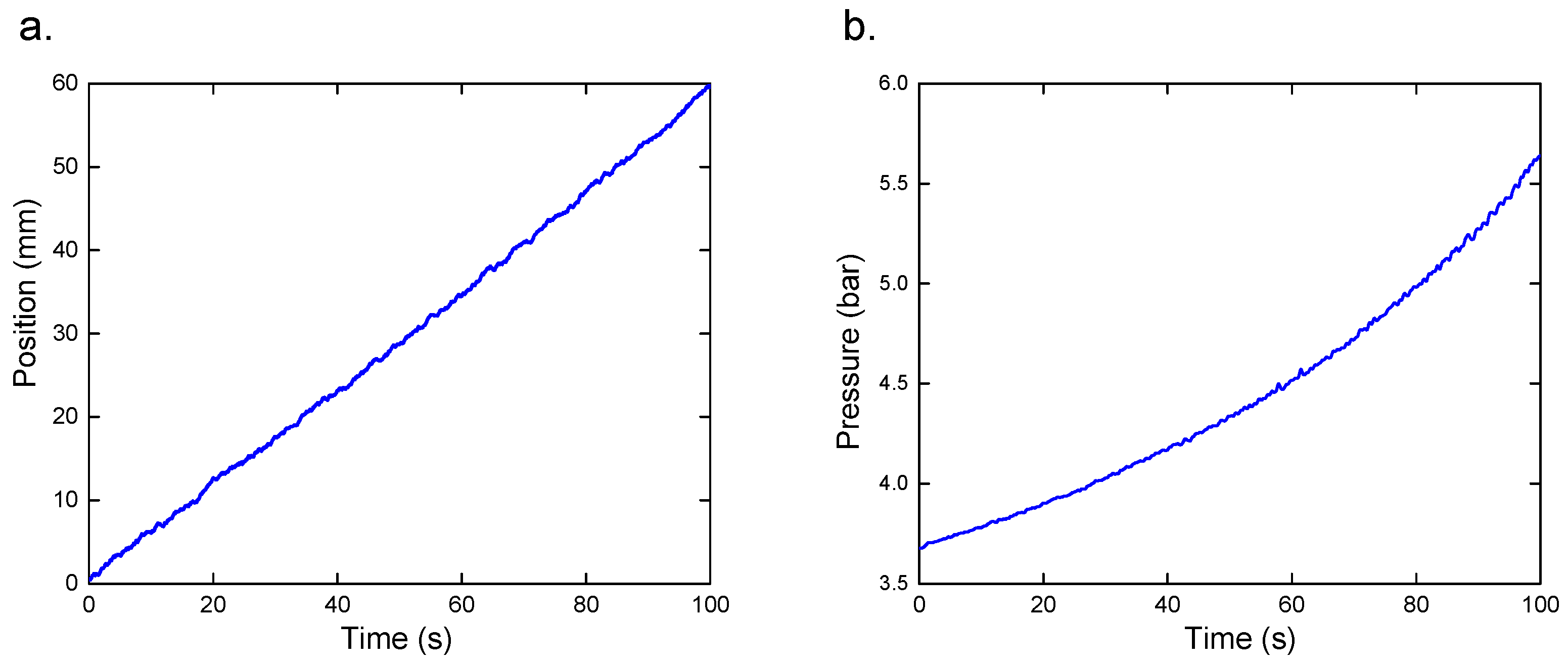
The compressed air force depends on the thermodynamic parameters as well as the structural parameter of PAM such as the working volume and contracted length of the muscle tube. In order to validate the working volume, the experiment is realized as follows: The air pressure inside the bladder is increased to the value of 3.7 bar through the pressure regulator. The length of the PAM is shrunk to approximately 20% of the natural length (60 mm). Then, the free end of the PAM is moved slowly (0.6 mm/s) thanks to the pneumatic excited system. The result is used to obtain the time history of the position and pressure, as shown in Figure 7. Due to very slow movement of the pneumatic cylinder, the thermodynamic state of air inside of the bellow is an isothermal process; hence, the polytropic exponent (n) is equal to 1. The result is used to obtain the experimental curve of the volume of the PAM plotted by the dashed line in Figure 8. In addition, the theoretical curve of the volume is calculated by using Equation (4), in which the initial fiber angle of 28.6° is plotted by the solid line. It is noteworthy to observe that the calculated result follows the experiment well. The result confirmed that the curve of the bellow volume versus the contracted length of the PAM is nonlinear. Accordingly, the theoretical model makes it effective and feasible to analyze the complex stiffness of the PAM.
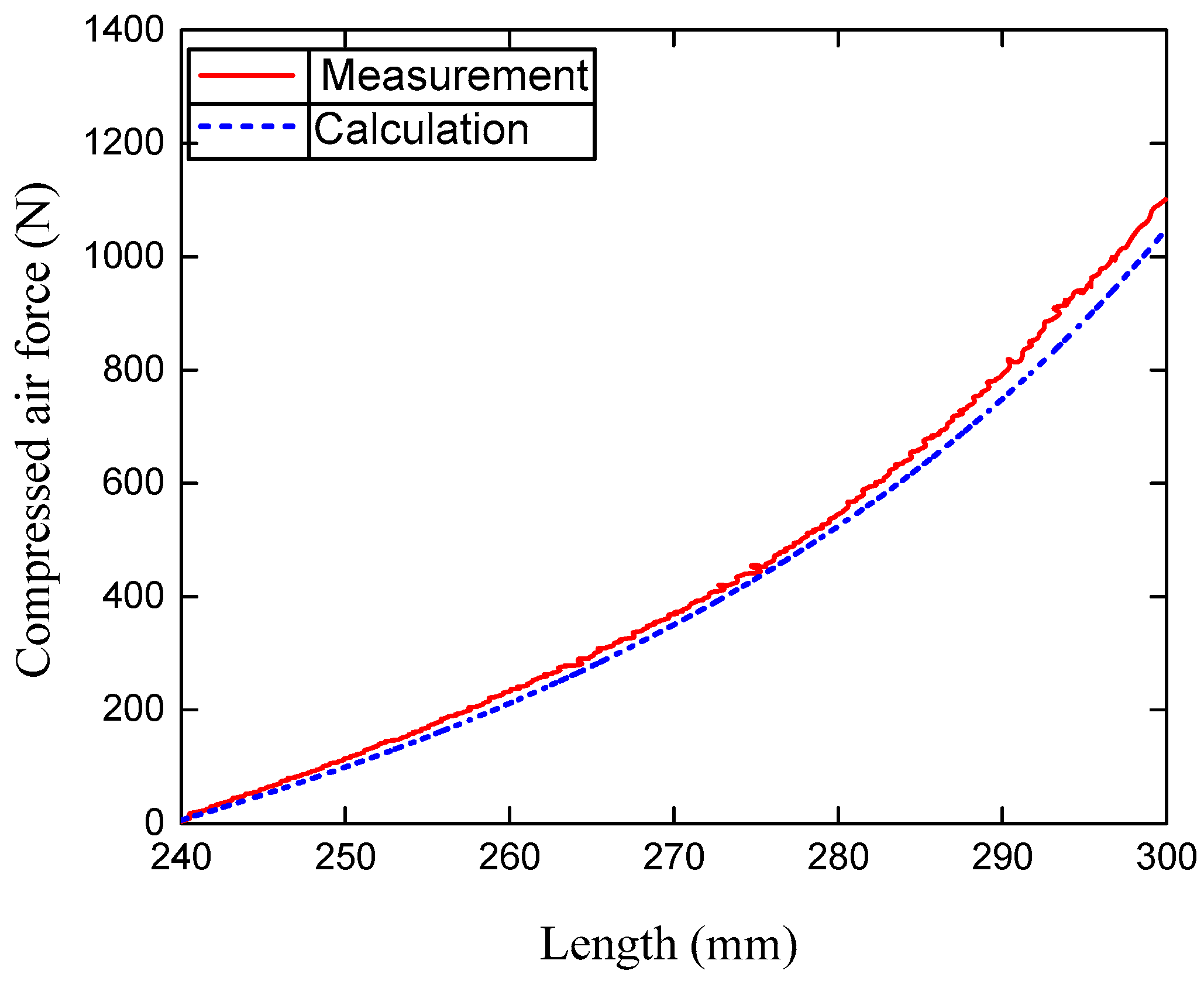
From the validation of the predicted model of the working volume, the theoretical model of the compressed air force, which is calculated by Equation (5) in which the inner pressure of the bellow is determined by Equation (2), will be compared with the experimental data. Here, the experimental condition is the same as in Figure 8. It can be observed in Figure 9 that the calculated force is lower than the experimental data. This is evident because the predicted model in Equation (5) ignored the viscoelastic force of the rubber material. But the trend of the calculated curve tracks the experimental data. Furthermore, the experiment as well as calculation results indicated that the air compressed force offers a nonlinear curve versus the contracted length of the PAM.
b.
Restoring model of the PAM
The bladder is pressured to 3 bar; then, the pushing force generated by the PAM is controlled according to the harmonic signal with the amplitude of 150 N and various frequencies comprising 1, 2, 3…, 10 Hz. Minimizing the cost function (16) is performed based the water cycle algorithm, resulting in obtaining a set of the optimal parameters of the fractional Maxwell model, including α = 0.27; β = 49.82; Ke = 2260. The convergence of the cost function with respect to the iteration is shown in Figure 10. It is interesting that the cost function is converged to zero after 20 iterations.
+ First study case: the change in amplitude
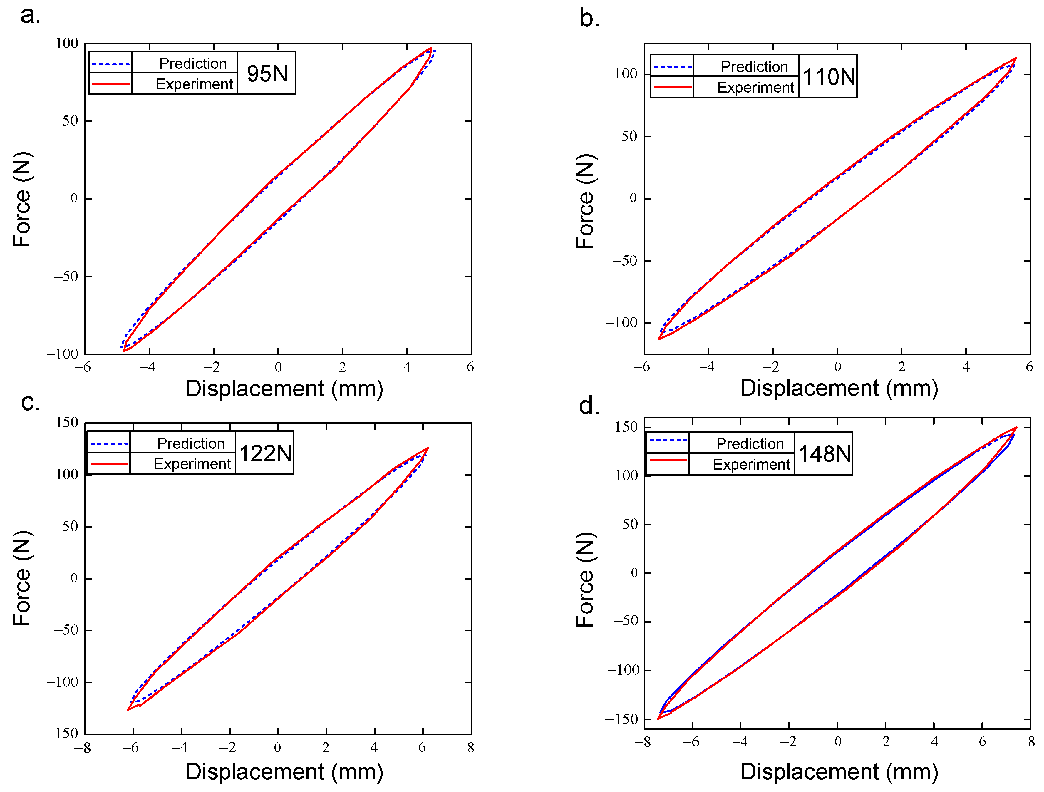
The PAM is excited at the frequency of 3.5 Hz and four force amplitudes, including 95, 110, 122 and 148 N. The predicted and experimental force hysteresis curves are plotted in Figure 11 (a detailed annotation of line types is presented in the upper-left corner panel of the figure). It is noteworthy to see that although the predicted results have errors compared with the experimental data, the predicted hysteresis curve can well capture the experimental curve. The force amplitude is increased according to the development of the displacement amplitude.
+ Second study case: The change in frequency
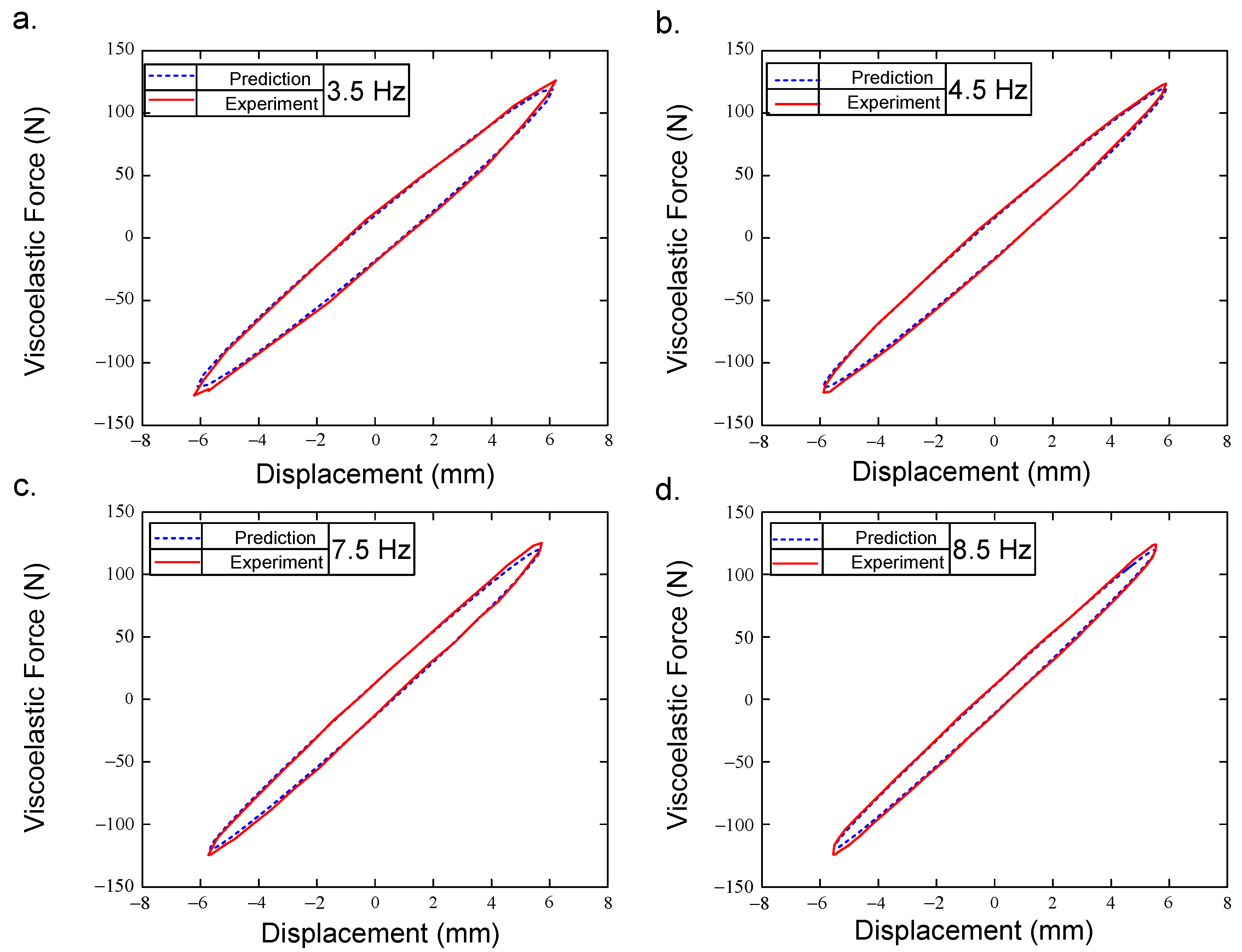
One again, the force amplitude of 125 N and excited frequencies involving 3.5, 4.5, 7.5 and 8.5 Hz are investigated. The result is used to obtain the force–displacement loop for these four excited frequencies. Figure 12 shows the solid lines present for the experimental curve; meanwhile, the simulation curve is plotted by the dashed line. It concludes that the overall trend between the prediction and experiment is the same. The experiment as well as simulation indicated that when the excited frequency is increased, the displacement amplitude is reduced, which means that the dynamic stiffness of the PAM is increased along with the increase in the frequency. Furthermore, it can be seen from Figure 12 that the force–displacement loop is narrowed according to the development of the frequency. This reveals undoubtedly that the higher the excited frequency, the more the effects of the frequency on the hysteresis curve are reduced.

5. Conclusions

This paper developed a restoring model of a commercial PAM based on McKibben’s structure. The fractional Maxwell for describing the viscoelasticity of the rubber tube of the PAM was proposed. The cost function was built through the equation of the hysteresis loop. The optimal parameters of the proposed model were identified by using the water cycle algorithm. The studied result concluded that the proposed model matches well with the experimental data, although there are small deviations. Then, the effects of the viscoelastic property of the rubber material on the dynamic response of the PAM were investigated, confirming that increasing the excited frequency leads to a reduction in the effects of the frequency on the hysteresis curve. The studied model is a suitable tool in the field of the system vibration analysis using PAM as an elastic element actuator. Experimental and predicted results indicated that the force–displacement loop is dependent on the force amplitude and frequency.

Author Contributions

Conceptualization, M.K.N.; methodology, V.C.T.; validation, T.D.L. and N.Y.P.V.; formal analysis, V.C.T.; investigation, M.K.N. and T.D.L.; writing—original draft, N.Y.P.V. and V.C.T.; visualization, T.D.L.; supervision, T.D.L.; project administration, M.K.N. All authors have read and agreed to the published version of the manuscript.

Funding

This work belongs to the project grant No: T2024−02 funded by the Ho Chi Minh City University of Technology and Education, Vietnam.

Data Availability Statement

The data presented in this study are available on request from the corresponding author.

Conflicts of Interest

The authors declare no conflicts of interest.

References

  1. Xiao, W.; Hu, D.; Chen, W.; Yang, G.; Han, X. Modeling and analysis of bending pneumatic artificial muscle with multi-degree of freedom. Smart Mater. Struct. 2021, 30, 095018. [Google Scholar] [CrossRef]
  2. Lin, C.-J.; Sie, T.-Y.; Chu, W.-L.; Yau, H.-T.; Ding, C.-H. Tracking control of pneumatic artificial muscle-activated robot arm based on sliding-mode control. Actuators 2021, 10, 66. [Google Scholar] [CrossRef]
  3. Zhang, Y.; Cheng, Q.; Chen, W.; Xiao, J.; Hao, L.; Li, Z. Dynamic modeling and inverse compensation for coupled hysteresis in pneumatic artificial muscle-actuated soft manipulator with variable stiffness. ISA Trans. 2024, 145, 468–478. [Google Scholar] [CrossRef]
  4. Xie, S.Q.; Jamwal, P.K. An iterative fuzzy controller for pneumatic muscle driven rehabilitation robot. Expert Syst. Appl. 2011, 38, 8128–8137. [Google Scholar] [CrossRef]
  5. Liu, Q.; Zuo, J.; Zhu, C.; Xie, S.Q. Design and control of soft rehabilitation robots actuated by pneumatic muscles: State of the art. Future Gener. Comput. Syst. 2020, 113, 620–634. [Google Scholar] [CrossRef]
  6. Nguyen, H.T.; Trinh, V.C.; Le, T.D. An Adaptive Fast Terminal Sliding Mode Controller of Exercise-Assisted Robotic Arm for Elbow Joint Rehabilitation Featuring Pneumatic Artificial Muscle Actuator. Actuators 2020, 9, 118. [Google Scholar] [CrossRef]
  7. Tomori, H.; Midorikawa, Y.; Nakamura, T. Vibration control of an artificial muscle manipulator with a magnetorheological fluid brake. In Proceedings of the 13th International Conference on Electrorheological Fluids and Magnetorheological Suspensions, Ankara, Turkey, 2–6 July 2012. [Google Scholar]
  8. Kalita, B.; Leonessa, A.; Dwivedy, S.K. A Review on the Development of Pneumatic Artificial Muscle Actuators: Force Model and Application. Actuators 2022, 11, 288. [Google Scholar] [CrossRef]
  9. Lin, C.J.; Lin, C.R.; Yu, S.K.; Chen, C.T. Hysteresis model and tracking control for a dual pneumatic artificial muscle systems using Prandtl-Ishlinskii model. Mechatronics 2014, 28, 35–45. [Google Scholar] [CrossRef]
  10. Xie, S.L.; Liu, H.T.; Mei, J.P.; Gu, G.Y. Modeling and compensation of asymmetric hysteresis for pneumatic artificial muscles with a modified generalized Prandtl-Ishlinskii model. Mechatronics 2018, 52, 49–57. [Google Scholar] [CrossRef]
  11. Tri, V.N.; Kamers, B.; Romon, H.; Brussel, H.V. Characterization of hysteresis in a pneumatic muscle manipulatot with accounting for the creep effect. IFAC Proc. Vol. 2010, 43, 296–302. [Google Scholar] [CrossRef]
  12. Sarosi, J. Elimination of the hysteresis effect of PAM actuator: Modeling and experimental studies. Teh. Vjesn.-Tech. Gaz. 2015, 22, 1489–1494. [Google Scholar]
  13. Mohareb, S.A.; Alsharkawi, A.; Zgoul, M. Hysteresis modeling of a PAM system using ANFIS. Actuators 2021, 10, 280. [Google Scholar] [CrossRef]
  14. Luo, X.; Xia, M.; Ding, Y.; Ding, H. Hysteresis modeling and compensation of a pneumatic end-effector based on Gaussian process regression. Sens. Actuators A Phys. 2020, 315, 112227. [Google Scholar] [CrossRef]
  15. Shakiba, S.; Ourak, M.; Poorten, E.V.; Ayati, M.; Yousefi-Koma, A. Modeling and compensation of asymmetric rate-dependent hysteresis of a miniature pneumatic artificial muscle-based catheter. Mech. Syst. Signal Process. 2021, 154, 107532. [Google Scholar] [CrossRef]
  16. Kalita, B.; Dwivedy, S.K. Nonlinear dynamics of a parametrically excited pneumatic artificial muscle (PAM) actuator with simultaneous resonance condition. Mech. Mach. Theory 2019, 135, 281–297. [Google Scholar] [CrossRef]
  17. Srosi, J.; Biro, I.; Nemeth, J.; Cveticanin, L. Dynamic modeling of a pneumatic muscle actuator with two-direction motion. Mech. Mach. Theory 2015, 85, 281–297. [Google Scholar] [CrossRef]
  18. Doumit, M.; Leclair, J. Development and testing of stiffness model for pneumatic. Int. J. Mech. Sci. 2017, 120, 30–41. [Google Scholar] [CrossRef]
  19. Zhang, Y.; Liu, H.; Ma, T.; Hao, L.; Li, Z. A comprehensive dynamic model for pneumatic artificial muscles considering different input frequencies and mechanical loads. Mech. Syst. Signal Process. 2021, 148, 107133. [Google Scholar] [CrossRef]
  20. Guan, Q.; Sun, J.; Liu, Y.; Wereley, N.M.; Leng, J. Characterization and nonlinear models of bending extensile/contractile pneumatic artificial muscles. Smart. Mater. Struct. 2021, 30, 025024. [Google Scholar] [CrossRef]
  21. Saito, N.; Satoh, T.; Saga, N. Double Air Chambers Pneumatic Artificial Muscle and Non-Hysteresis Position Control. Actuators 2024, 13, 282. [Google Scholar] [CrossRef]
  22. Dunn, L. Introduction to viscoelasticity in polymers and its impact on rolling resistance in pneumatic tyres. Int. J. Squiggly Wobbly Mater. 2019, 23, 1–8. [Google Scholar]
  23. Shitikova, M.V.; Krusser, A.I. Models of viscoelastic materials: A review on historical development and formulation. In Theoretical Analyses, Computations, and Experiments of Multiscale Materials; Springer: Cham, Switzerland, 2022. [Google Scholar]
  24. Perkins, J.N.; Lach, T.M. Viscoelasticity: Theories, Types and Models; Nova Science Publishers: Hauppauge, NY, USA, 2011. [Google Scholar]
  25. Fatima, I.D.; Shafi, N.; Anjum, H. Viscoelastic properties of rubber material modeling. In Proceedings of the 2019 International Conference on Applied and Engineering Mathematics (ICAEM), Taxila, Pakistan, 27–29 August 2019. [Google Scholar]
  26. Berg, M. A model for rubber springs in the dynamic analysis of rail vehicles. Proc. Inst. Mech. Eng. Part F J. Rail Rapid Transit 1997, 211, 95–108. [Google Scholar] [CrossRef]
  27. Podlubny, I. Practional Differential Equations; Academic Press: Cambridge, MA, USA, 1999. [Google Scholar]
  28. Eskandar, H.; Sadollah, A.; Bahreininejad, A.; Hamdi, M. Water cycle algorithm—A novel metaheuristic optimization method for solving constrained engineering optimization problems. Comput. Struct. 2012, 110–111, 151–166. [Google Scholar] [CrossRef]
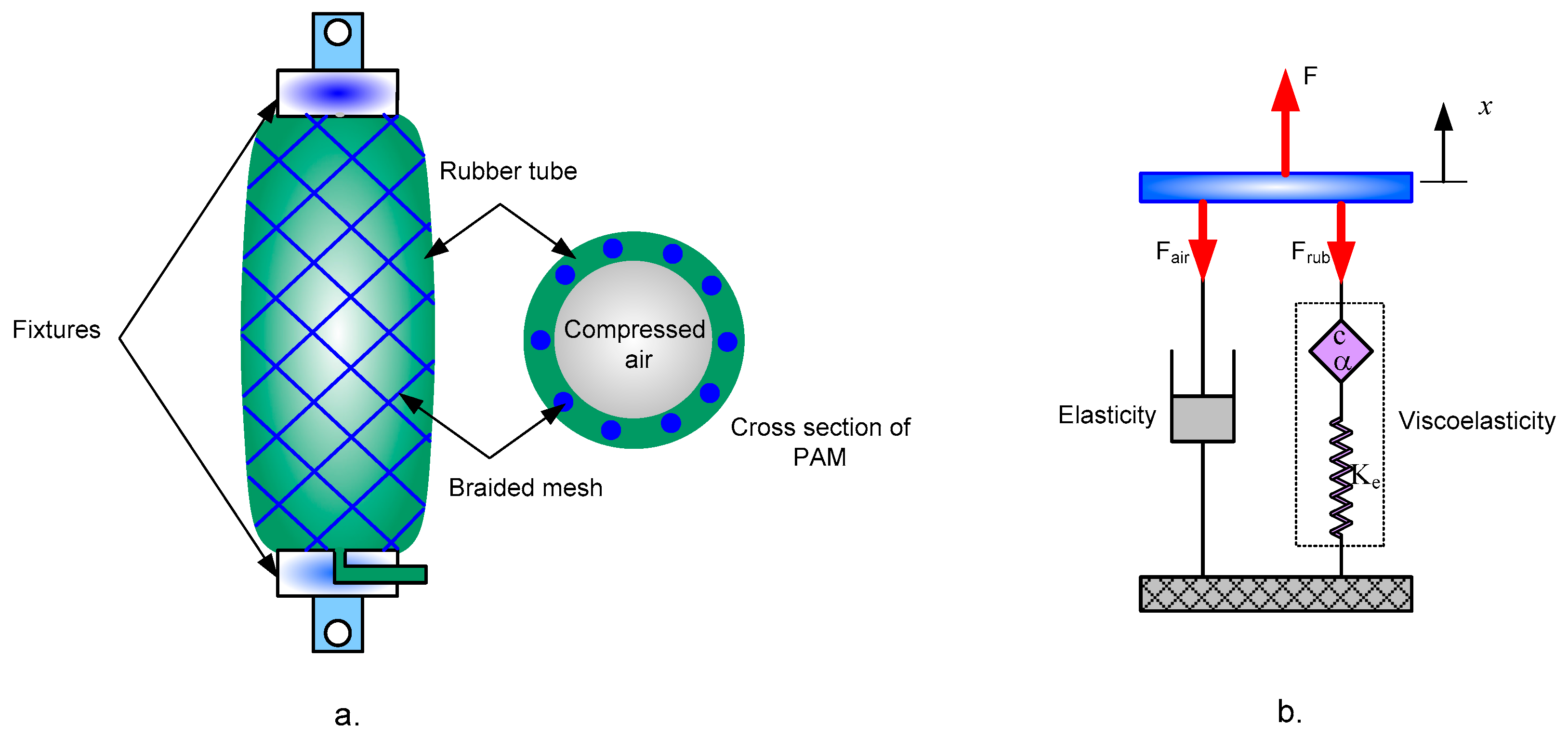
Figure 1. Physical structure of PAM (a); diagram of fractional Maxwell model (b).
Actuators 13 00355 g001
Figure 2. Working states of the PAM.
Actuators 13 00355 g002
Figure 3. Hysteresis curve of fractional Maxwell model.
Actuators 13 00355 g003
Figure 4. Hydrological cycle.
Actuators 13 00355 g004
Figure 5. The schematic diagram of the stream to river and river to sea.
Actuators 13 00355 g005
Figure 6. Experimental setup (a); diagram of the apparatus (b): 1—Motor; 2—Compressor; 3—Filter; 4—Air reservoir; 5—Pressure regulator; 6—On–off valve; 7—Pressure gauge; 8—Safety valve; 9—Pressure sensor; 10—PAM; 11—Loadcell; 12—Position sensor; 13—Base; 14—Coupling; 15—Pneumatic cylinder; 16—Proportional valve; 17—NI card 6221; 18—Computer.
Actuators 13 00355 g006
Figure 7. Measured signals versus time: (a) pressure; (b) position.
Actuators 13 00355 g007
Figure 8. Comparison between the experimental and approximate curves.
Actuators 13 00355 g008
Figure 9. Comparison between the simulation and experiment (detailed annotation of the line types is presented in top-left corner panel).
Actuators 13 00355 g009
Figure 10. Convergence of the cost function.
Actuators 13 00355 g010
Figure 11. Comparison of experimented and calculated hysteresis loops with frequency of 3.5 Hz and various force amplitudes: (a) 95 N; (b) 110 N; (c) 122 N; (d) 148 N.
Actuators 13 00355 g011
Figure 12. Comparison of experimented and calculated hysteresis loops with force amplitude of 125 N and various frequencies: (a) 3.5 Hz (b) 4.5 Hz; (c) 7.5 Hz; (d) 8.5 Hz.
Actuators 13 00355 g012
Table 1. Water cycle algorithm.
Step 1: Select the initial parameters including: Nriver—number of rivers; dmax—a small number (close to zero); Npop—population size.
Step 2: Generate random initial population (Npop) and number of initial streams (Nstream), rivers(Nriver) and sea.
N p o p = S t r e a m 1 S t r e a m 2 S t r e a m i S t r e a m N p o p T
with S t r e a m i = x 1 i x 2 i x n i ; n is the number of design variables,
N stream = N p o p N r i v e r + 1 s e a
Step 3: Calculate the value of the fitness function for each stream by using Equation (16).
Step 4: Determine the intensity calculation of flow for sea and river.
N S n = r o u n d F i t n F i t N r i v e r + 2 i = 1 N r i v e r + 1 F i t i × N s t r e a m s ;   i = 1 , 2 , , N r i v e r + 1
Step 5: Streams flow to river and rivers flow to sea
X s t r e a m i + 1 = X s t r e a m i + r a n d   ×   C i ×   X r i v e r i X s t r e a m i X r i v e r i + 1 = X r i v e r i + r a n d   ×   C i ×   X s e a i X r i v e r i C i = 2 1 i max ( i l t e r a t i o n ) 2
Step 6: Exchange the position of the stream and river and the position of the river and sea
     If the fitness function of the stream is lower than that of the river
        Exchange position of stream and river
     end
     If the fitness function of the river lower than that of the sea
        Exchange position of river and sea
     end
Step 7: Check evaporation condition among sea and river
X s e a X r i v e r i < d max ,   i = 1 , , N r i v e r
If the evaporation condition is satisfied
   Creation of clouds and rain by
X s t r e a m n e w = X s t r e a m + μ   ×   r a n d ( 1 , n )
end
with a coefficient showing the range of the searching region near the sea.
Step 8: Check evaporation condition among sea and stream
X s e a X s t r e a m i < d max ,   i = 1 , , N s t r e a m
If the evaporation condition is satisfied
   Creation of clouds and rain by:
X s t r e a m n e w = X s t r e a m + μ   ×   r a n d ( 1 , n )
end
Step 9: Reduce the value of d max by using
d max i + 1 = d max i d max i max ( i l t e r a t i o n )
Step 10: Check the convergence condition. If the convergence condition is satisfied, the algorithm will be stopped to obtain the optimal solution; otherwise return to step 5.
Disclaimer/Publisher’s Note: The statements, opinions and data contained in all publications are solely those of the individual author(s) and contributor(s) and not of MDPI and/or the editor(s). MDPI and/or the editor(s) disclaim responsibility for any injury to people or property resulting from any ideas, methods, instructions or products referred to in the content.