Abstract
When a robot performs tasks such as assembly or human–robot interaction, it is inevitable for it to collide with the unknown environment, resulting in potential safety hazards. In order to improve the compliance of robots to cope with unknown environments and enhance their intelligence in contact force-sensitive tasks, this paper proposes an improved admittance force control method, which combines classical adaptive control and machine learning methods to make them use their respective advantages in different stages of training and, ultimately, achieve better performance. In addition, this paper proposes an improved Deep Deterministic Policy Gradient (DDPG)-based optimizer, which is combined with the Gaussian process (GP) model to optimize the admittance parameters. In order to verify the feasibility of the algorithm, simulations and experiments are carried out in MATLAB and on a UR10e robot, respectively. The experimental results show that the algorithm improves the convergence speed by 33% in comparison to the general model-free learning method, and has better control performance and robustness. Finally, the adjustment time required by the algorithm is 44% shorter than that of classical adaptive admittance control.
1. Introduction
As industrial robot applications continue to expand [1,2,3], the operational process of industrial robots has become increasingly independent of human intervention. It is imperative that robots possess the capacity to interact with their environments in a stable and reliable manner. However, in environments with high complexity and uncertainty, it remains challenging to ensure the reliable and accurate interactive control of the robot [4]. The models of commercial robots are highly precise [5], but the precise modeling of the environment is usually not available. The occurrence of sudden changes in the environment can result in the generation of unpredictable deviations in the interaction.
Compliance control is widely used in robot interaction control [6]. This kind of method also pays attention to contact force tracking while performing position control. Common compliance control methods can be roughly classified as hybrid position/force control [7] and impedance control [8]. Position-based impedance control is also known as admittance control. The accuracy of hybrid position/force control is reduced because it ignores the dynamic coupling between the robot and the environment [9]. Impedance control establishes the dynamic relationship between robot motion and contact force, and can achieve very accurate control with simple modeling.
Adaptive control can effectively deal with the complex situation of uncertainty [10]. Adaptive impedance control is an extension of classical impedance control. It continuously adjusts the impedance parameters to adapt to dynamic changes through feedback information, showing higher flexibility and robustness. So far, there have been many research results on such algorithms [11,12,13,14].
With the rapid development of artificial intelligence technology, machine learning methods are gradually being applied to robot force control technology. Compared with classical control, intelligent control is more inclusive of the unknowns in the model. In the early days, imitation learning method was used to build the model by collecting the demonstration experience of human experts [15,16,17,18,19]. A neural network was used for parameter estimation [20], contact force prediction [21] and system unknowns prediction [22,23]. Imitation learning was used to improve the portability of the controller [24]. In recent years, neural networks have received more attention, and their application to variable impedance control has also been widely developed [25,26,27,28].
Reinforcement learning (RL) is another machine learning technique. Unlike deep learning, which relies on a large amount of prior knowledge, reinforcement learning is semi-supervised learning. It accumulates experience through repeated attempts to achieve autonomous learning. In [29], the prior knowledge of the operator is introduced, and the reinforcement learning, fuzzy technology, and neural network are combined to propose a reinforcement learning fuzzy neural network architecture based on the actor–critic architecture, which is used to learn the parameters of the variable admittance controller. In [30], the artificial neural network is used to establish the dynamics of human–computer interaction, and the model is used for reinforcement learning, combining a cross-entropy method and model prediction control. In [31], a policy iteration with constraint embedding is proposed to ensure the semi-definiteness of the policy evaluation function and to simplify its form. In [32], the admittance parameters are directly updated through Q-learning. In [33], a reinforcement learning variable impedance control with stability guarantee is proposed. The extended cross-entropy reinforcement learning method is trained to make direct decisions on the state variables. Its stability comes from the conservative design based on the stability of the constant impedance controller. In [34,35], model-based reinforcement learning methods are used to approximate the system’s environmental change model to predict the evolution of the system state in the future.
Usually, the law of environmental change is unknown to the optimizer. In practice, environmental changes are usually estimated by designing dynamic models or designing model-free reinforcement learning to directly approximate the state results after environmental changes. The difficulty in model-based reinforcement learning is that, due to uncertainty, a good dynamics model is usually difficult to design [36,37]. In model-free methods, the value function is directly synthesized, which requires a lot of training time and data.
Deep Deterministic Policy Gradient (DDPG) [38] is one of the reinforcement learning methods that is based on actor–critic architecture. It combines the advantages of the DQN algorithm and DPG algorithm. It not only solves the problem that random policy is difficult to sample in complex action space, but also makes up for the defect that DQN cannot deal with high-dimensional continuous action space. It is very suitable for applications with high dimensions and large task space such as robot operation.
The Gaussian process (GP) model is another kind of learner that has been combined with reinforcement learning [34,35,39,40]. Compared with other regression models, the GP model has a better approximating effect when the data set is smaller and contains the uncertainty of the model. Such characteristics are more suitable for relatively small changes during industrial robot operations. We use it to approximate the policy function to achieve the purpose of reducing the amount of data and fast convergence.
In this paper, an intelligent variable admittance control method, combining classical control theory and reinforcement learning theory, is proposed and applied to the interactive compliance control of industrial robots in a changing environment. By fully considering the results of classical control and an intelligent optimizer, the parameters of impedance control are adjusted, which improves the limitation of the model-free reinforcement learning method. This method does not need to model the complex physical environment and robot, and does not require long-term experience accumulation, which improves safety and learning efficiency. The GP model is combined with the DDPG in the reinforcement learning system and applied to the approximation policy function. The improved algorithm requires fewer data sets and hyperparameters, and has higher learning efficiency and faster convergence.
The rest of this paper is as follows: Section 2 introduces the classical admittance control and states the problems to be studied. Section 3 describes the variable admittance control algorithm proposed in this paper in detail. Section 4 shows the results of simulations and experiments in detail. Finally, in Section 5, we summarize the research results of this paper.
2. Problem Statement
2.1. Classical Admittance Control
Hogan [8] proposed impedance control. The core idea of impedance control is to model the control object as a system with spring–mass–damping characteristics, and the relationship between contact force and motion state is characterized by the dynamic equation, so as to realize the control of the dynamic relationship between the two. In Cartesian space, the typical impedance model of a robot is expressed as
(n is the dimension of the minimal coordinate set) represent the mass, damping, and stiffness of the assumed system, which are positive definite. are the reference trajectory and the corrected trajectory; , are their velocity and acceleration, respectively. is the actual contact force / torque, and is the expected one.
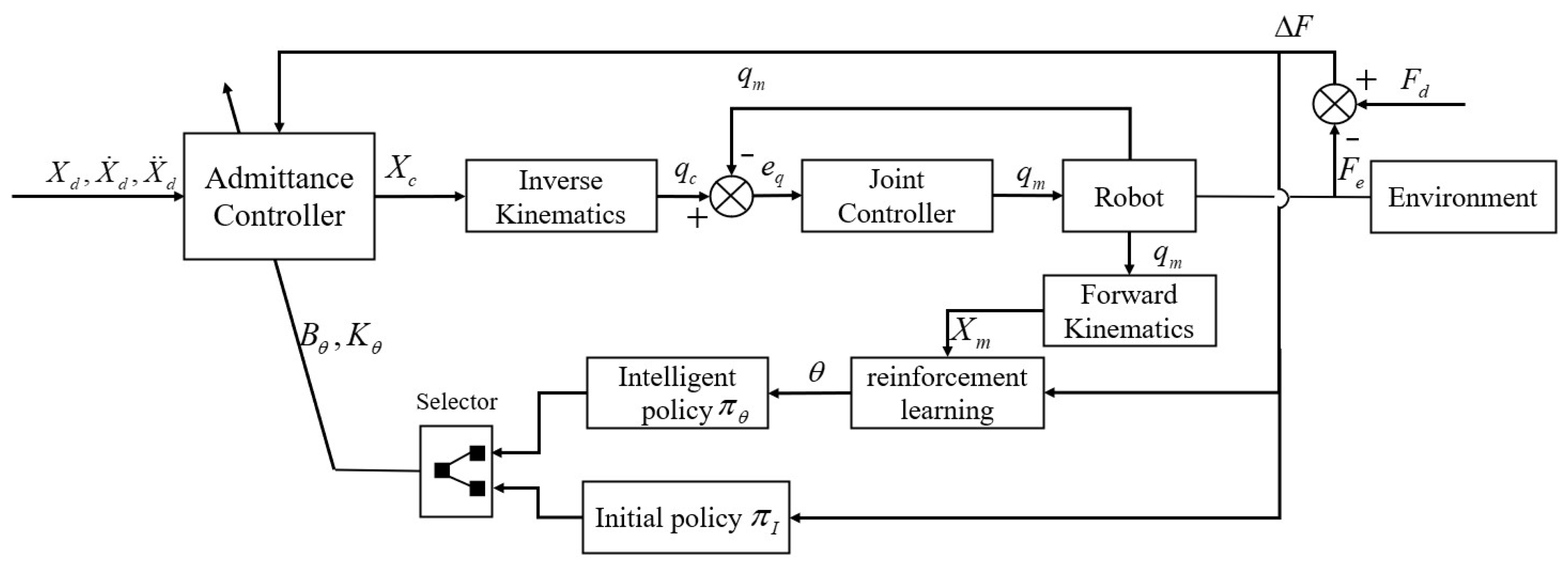
Admittance control is impedance control based on motion, which realizes the mapping from generalized force to generalized position. In general, the structure consists of a force control outer loop and a position control inner loop, as shown in Figure 1. The force controller receives the feedback from the force sensor, and outputs the corrected trajectory . After inverse kinematics mapping, the joint trajectory is tracked by the joint controller inner loop. Nowadays, compared with the constant parameter admittance control method, the admittance control of variable parameters must be developed to meet the increasingly complex work requirements.

Figure 1.
Classical admittance control system structure.
2.2. Evolution of Contact Force
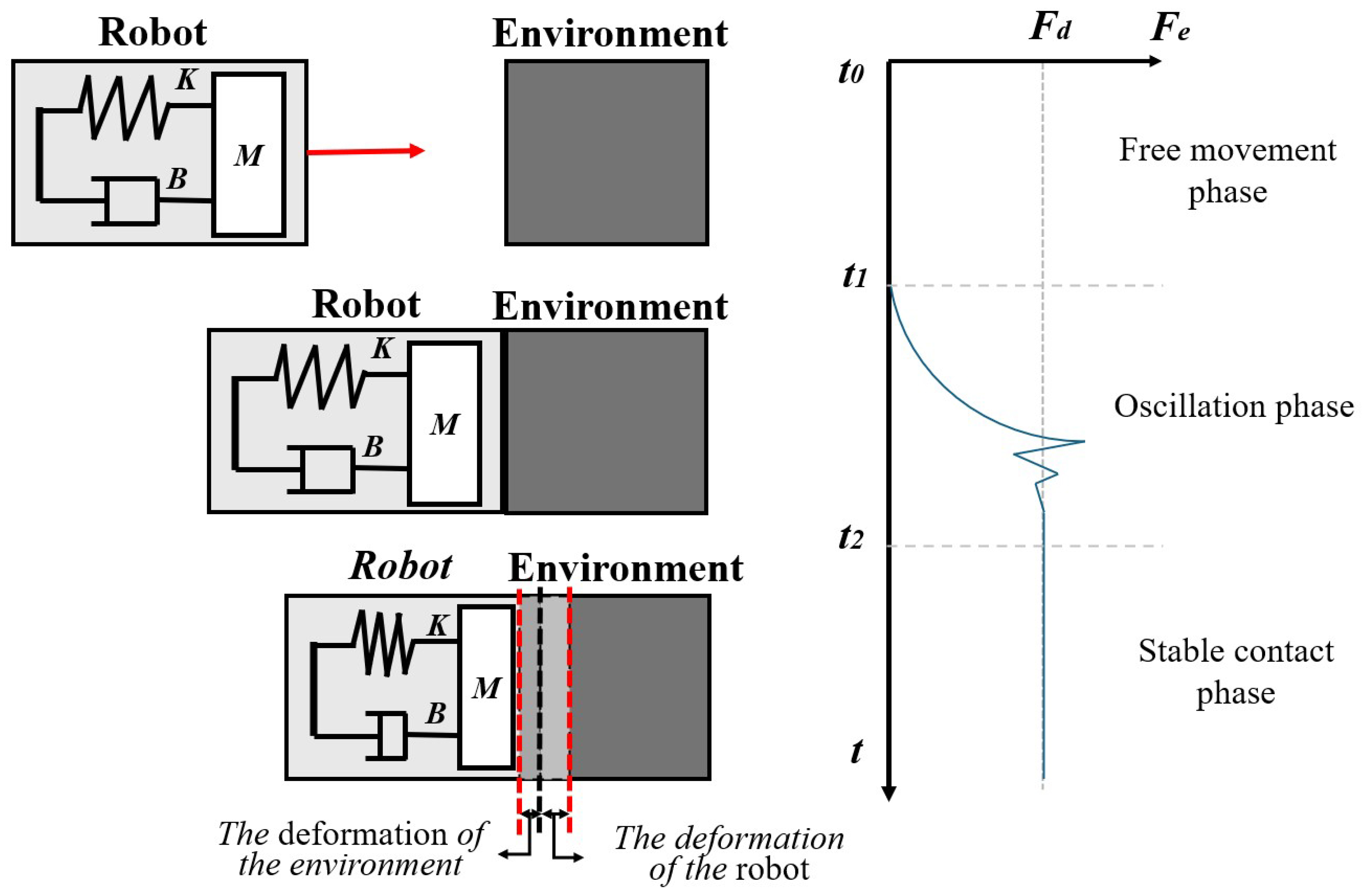
We model the robot as an admittance model with a multi-dimensional spring–mass–damping system. In general, the contact between the robot and the environment is divided into three phases, as shown in Figure 2.
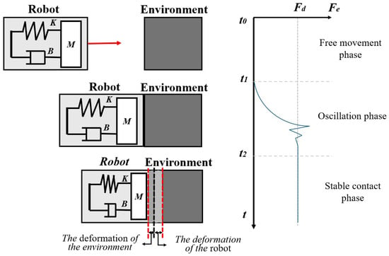
Figure 2.
Robot and environment contact process model.
On the left side of Figure 2, a schematic diagram of three phases is shown, and, on the right side, the evolution of contact force in different phases is shown. In the free movement phase, the robot has not been in contact with the environment. At this time, the contact force ; the admittance model changes the trajectory under the guidance of and gradually drives the robot to move in the direction of . In the oscillation phase, the robot has a strong nonlinear collision with the environment because the location and characteristics of the environment are unknown to the control system. However, due to the adjustment of the trajectory by the admittance control, such oscillations will gradually converge. In the stable contact phase, the contact force between the two tends to be stable, and .
In the oscillation phase of contact, the high force overshoot is not expected. At the same time, we hope that the contact force can quickly stabilize and make the steady-state error tend to zero. The following part of the paper will introduce the research on achieving this goal.
3. The Proposed Method
In this paper, an intelligent variable admittance control method is designed. In this method, the classical adaptive admittance controller is used as the initial policy to generate the previous experience (similar to the experience of human experts), in combination with a variable admittance controller trained by a reinforcement learning method (intelligent policy).
3.1. Intelligent Admittance Control System
As shown in Figure 3, the selector outputs variable admittance parameters by selecting two policies. For security, in the early phase of training, it tends to select the action generated by the initial policy and record the generated data set; after a period, the transformation from selecting the initial policy to selecting the learning policy is realized. In Figure 3, , and are defined as Equation (1). are the variable admittance parameters designed in this paper. , are the intelligent policy and initial policy, respectively, and is the joint variable of solved by inverse kinematics. After the adjustment of the robot joint controller, the real joint position of the robot is , while is the forward kinematics solution of .
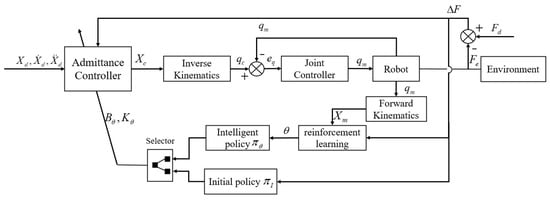
Figure 3.
Intelligent admittance control system structure.
3.2. The Establishment of Robot Model and Environment Model
The task environment is modeled as a first-order linear system (a linear spring):
where is the environmental position; the definition of is the same as Equation (1).
The robot is modeled as a classical admittance model, as shown in Equation (1). Suppose that the trajectory tracking error of the joint controller is zero, i.e., . Let and ; then, the admittance formula of the robot can be written as
With E as the output and as the input, the second-order system shown in Equation (3) has a transfer function . is expected to gradually approach 0; for , there is
When the system is in contact steady state, it has . The force error is expressed as
To make , we need to satisfy
Under the uncertainty conditions considered in this paper, Equation (6) cannot be satisfied directly due to the unknown values of and , and the steady state of the force error will always exist. To reduce the error, the disturbance caused by environmental uncertainty must be considered. It is assumed that the disturbance caused by environmental changes, including deformation caused by contact force, is and the disturbance of interaction force caused by is . Let and ; then, it becomes
, , and are classical admittance parameters that are constant. Next, variable admittance parameters are designed to compensate for the disturbance. It should be noted that the change in is not conducive to the stability of the system [13]. Thus, in this paper, we do not consider changing it. Let the variable admittance parameters be and ; then, it becomes
Let , then holds when .
3.3. Intelligent Policy
The intelligent policy is a modeled as a learner of the damping parameter , which is modeled as a Gaussian process model. Suppose that the data set , where are the optimal/sub-optimal state–action pairs in the experience pool H, , , and is the action corresponding to . The Gaussian process is an exploration of . It is generally modeled as a normal distribution with zero mean, which is uniquely determined by the covariance function. Considering the independent and identically distributed noise , Y is denoted by
where is the covariance matrix and I is the identity matrix.
For , the noiseless prediction function can be expressed as
Under the condition of D, Y and satisfy the multivariate joint Gaussian distribution. From the Bayes Rule, we can obtain
At time t, for , is the state and the corresponding output of GP is . Then, takes the mean of the posterior distribution:
For each element in the covariance matrix , we select the squared exponential kernel function:
where are one-dimensional elements in X and , respectively. , are the hyperparameters of the kernel function. is the sample variance, and represents the Euclidean distance measure between features.
To ensure the exploration in the early stage, noise is introduced; then, is denoted by
where is a constant. In order to meet the stability conditions of the admittance system described in [41], is also limited as . is the hyperparameter of , which includes and the hyperparameter of the kernel function itself. , =, =, and .
3.4. Initial Policy
The initial policy of this paper adopts the adaptive control law designed in [13]. In that paper, it is assumed that the robot is decoupled; the single-dimensional control law is expressed as follows:
where the definition of , , are as in Section 3.2, i.e., of a one-dimensional form. is the one-dimensional damping initial value, is a time-varying quantity, t is the real time, is the sampling rate, and is the learning rate.
Through the compensation of the adaptive variable damping control law, is established at steady state. The stability of the control law has been proven by the author of that article. Although the classical adaptive admittance control law is more robust than the constant admittance control, the experiment shows that its effect is still limited.
3.5. Intelligent Admittance Policy Integrated with Classical Control
Finally, the policy of the intelligent admittance controller is defined as :
is a constant positive real number, and is a time-negative correlation function. When the training begins, is larger and has a large probability to choose the decision of . With the increase in training time, gradually decreases until completely tends to choose after the accumulation of training.
denotes the neighborhood of . Since the randomness of the GP model always exists, when the output of the intelligent policy enters the neighborhood of the expected value, a small probability of jitter events will inevitably occur. When the robot system tends to the steady state of contact, its acceleration and force error should be very close to 0. At this time, the classical adaptive admittance control is selected as a policy to ensure accuracy.
3.6. Policy Optimization: Modified DDPG Algorithm
In the actor–critic architecture of the classic DDPG, the actor is designed as a deterministic policy function , where , are the actions of agent and state of environmental at time , is the policy function, and is the parameter of . The critic is a value function used to evaluate the policy , and both actor and critic are fitted by a neural network. To correct the deviation caused by the self-iteration of a single network, DDPG sets the dual neural network model architecture of the target network , and online network , .
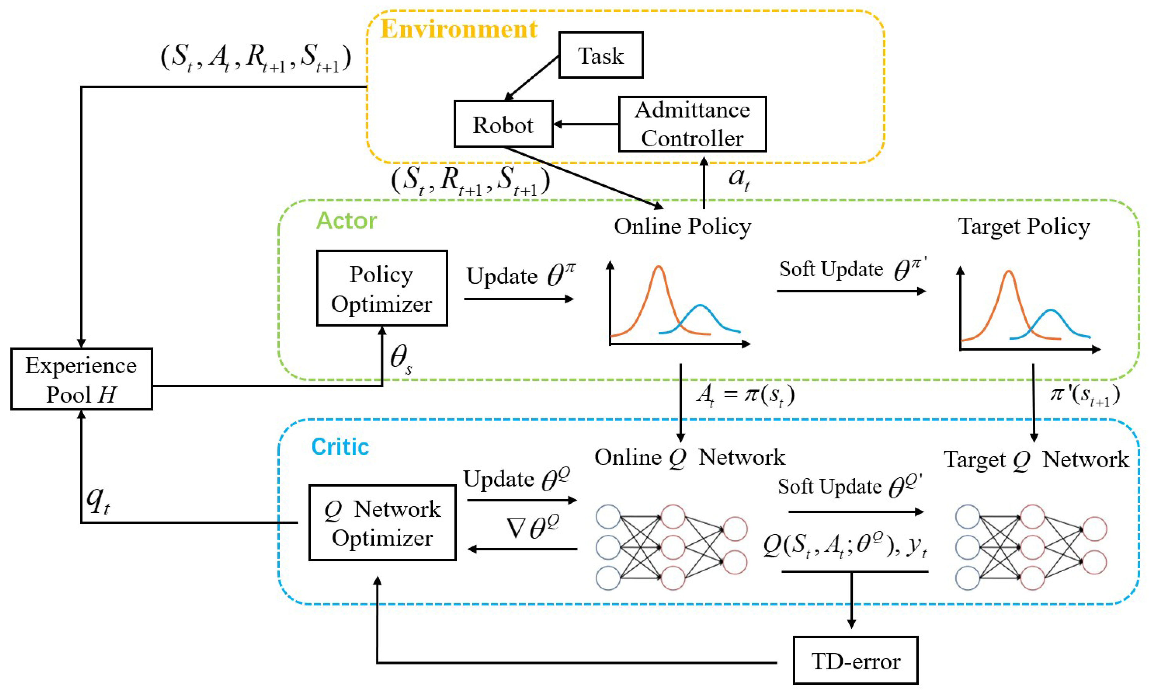
For , a modified DDPG algorithm is designed to optimize it, which is called the GP-DDPG algorithm. Specifically, is used as the actor in the DDPG, and the numerical method adapted to the GP model is used. The following describes the adaptive changes to DDPG.
As shown in Figure 4, the actor in this paper is , which outputs a uniquely determined action based only on and S. The critic, that is, the Q function is modeled as a neural network. The discrete time is , the state is , is the position vector of the end-effector in the Cartesian coordinates, is the velocity vector, and is the force/torque. , where is a simplified form of the output damping parameter, in which each element is composed of diagonals in the decoupled matrix form. For each state–action pair, the action value is calculated. The experience pool stores all historical data, which are used by the classical DDPG for experience playback, and, in this paper, they are also used to collect the hyperparameter .
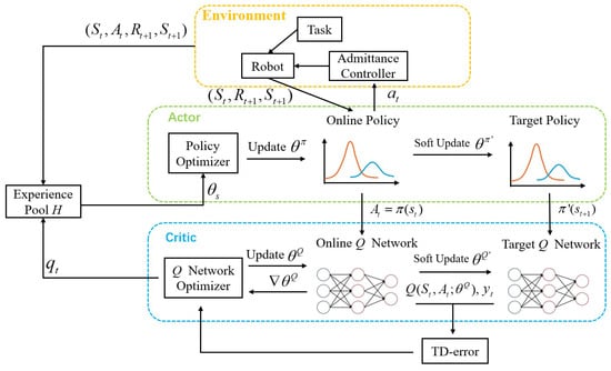
Figure 4.
The schematic diagram of the GP-DDPG algorithm.
The single-dimensional considers error consumption and energy consumption . It is expressed as follows:
where i in Equation (17) is the element of each dimension in the vector, denotes the restriction on the output, which has the same form as , and is a constant coefficient.
The optimization process of the objective function J is to find the optimal hyperparameter of , so as to obtain the optimal solution :
Different from the classical DDPG, the numerical method is used in this paper. As explained in Section 3.4, the hyperparameters of the policy function in this article are . The elite method is used for , and the maximum likelihood estimation (MLE) is used to obtain .
For , different from the traditional sampling method, the prior data of the GP in this paper uses the elite method to select the term with the greatest value from the experience pool H. Since has the exploratory property in multiple iterations, the sampling method in this paper still satisfies the random sampling condition. The choice of takes into account the value of the action in each experience , as well as the similarity between the state in which the experience is recorded and the current state .
is the indicator function, which selects elite samples with the best action value from H, is the Euclidean distance between the current state and the historical state, , are positive real numbers, and h is the historical experience in H. It should be noted that, to maximize the exploration rate, we update the value of the earlier data in H dynamically and randomly with the minibatch update of the critic network.
For , it is randomly initialized, and the optimization is completed by maximum likelihood estimation. In fact, the MLE is also a common method to deal with the hyperparameter optimization of Gaussian distribution.
The critic is used to estimate the of each in H to select elites as the hyperparameter set of the actor. In this way, the actor will be optimized along the direction of increasing Q. The optimization of the critic is similar to that of the classical DDPG using the gradient descent method:
Finally, the algorithm we proposed can be expressed as in Algorithm 1:
| Algorithm 1 GP-DDPG Algorithm Combined with Classical Control |
| 1: Initialize , , , Initialize action value network Initialize experience pool H 2: for episode = 1: M do 3: Receive initial observation state 4: for t = 0: T do 5: if or is in the neighborhood of zero 6: = 7: else 8: = 9: end if 10: Calculate , observe 11: Store transition in H 12: Get TD error with random minibatch of N transitions ; and soft update to 13: Calculate use for each and update use 14: Extract samples from H based on Equation (19) as 15: Get using MLE based on 16: end for 17: end for |
4. Results
The algorithm is simulated in MATLAB 2022b. In the simulation, the error of the position controller is ignored. Without any loss of generality, only one dimension of force control effect is verified in this paper. The single-dimension damping parameter output is limited to ; in is . For , there are , . , are single-dimensional mass parameter and spring parameter design, respectively.
4.1. Simulation Results
4.1.1. The Performance of the GP-DDPG Algorithm
Firstly, the learning performance of the proposed method is verified and compared with the method using only GP-DDPG (without initial policy); the necessity of the initial policy is proven. The robot task environment is shown in Figure 5. The base coordinate system is located on the robot base, and the end of effector is located on the X-O-Z plane, moving at a constant speed of 0.3 m/s in the Y direction. The environment is a plane , perpendicular to the motion direction of the robot. The stiffness of the plane is , the position of environmental is completely unknown to the robot, and the expected force in the Y direction is set to N.
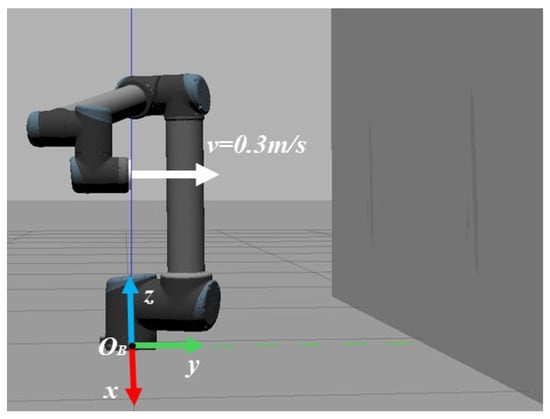
Figure 5.
Robot task environment. The environment is a vertical wall on the right side of the picture. It is assumed that there is no noise in the control process.
For , there are , . The Q network is designed as a full-connect neural network with three hidden layers; each layer has 64 neurons, and the initial weight is sampled from a Gaussian distribution.
Assuming that , the duration of a task is set to 15 s, and learnings are performed. The obtained learning results and evolution process are shown in Figure 6, Figure 7 and Figure 8. The addition of the classical algorithm provides experience for the learner. The whole algorithm shows a convergence trend. When , the output of tends to be stable. At this time, is still exploratory, and the fluctuation caused by bad trials is quickly corrected, which indicates that the robustness of the controller is gradually improved. After that, the performance of is further improved. When the contact force reaches the neighborhood of the expected steady-state error, it is switched to the classical adaptive controller, so that . After 10 instances of learning, the model can stabilize the contact force at .
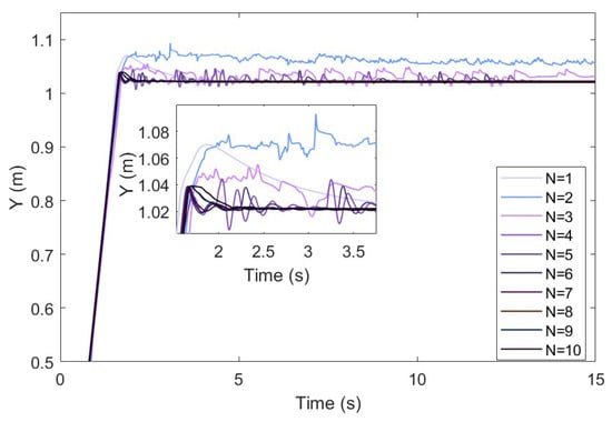
Figure 6.
Trajectory correction performance of the GP-DDPG algorithm with initial policy.

Figure 7.
Force-tracking performance of the GP-DDPG algorithm with initial policy: (a) The change in contact force in 1∼10 learnings; (b) N = 1∼5; (c) N = 5∼10.

Figure 8.
Damping variation performance of the GP-DDPG algorithm with initial policy: (a) The change in damping in 1∼10 learnings; (b) N = 1∼5; (c) N = 5∼10.
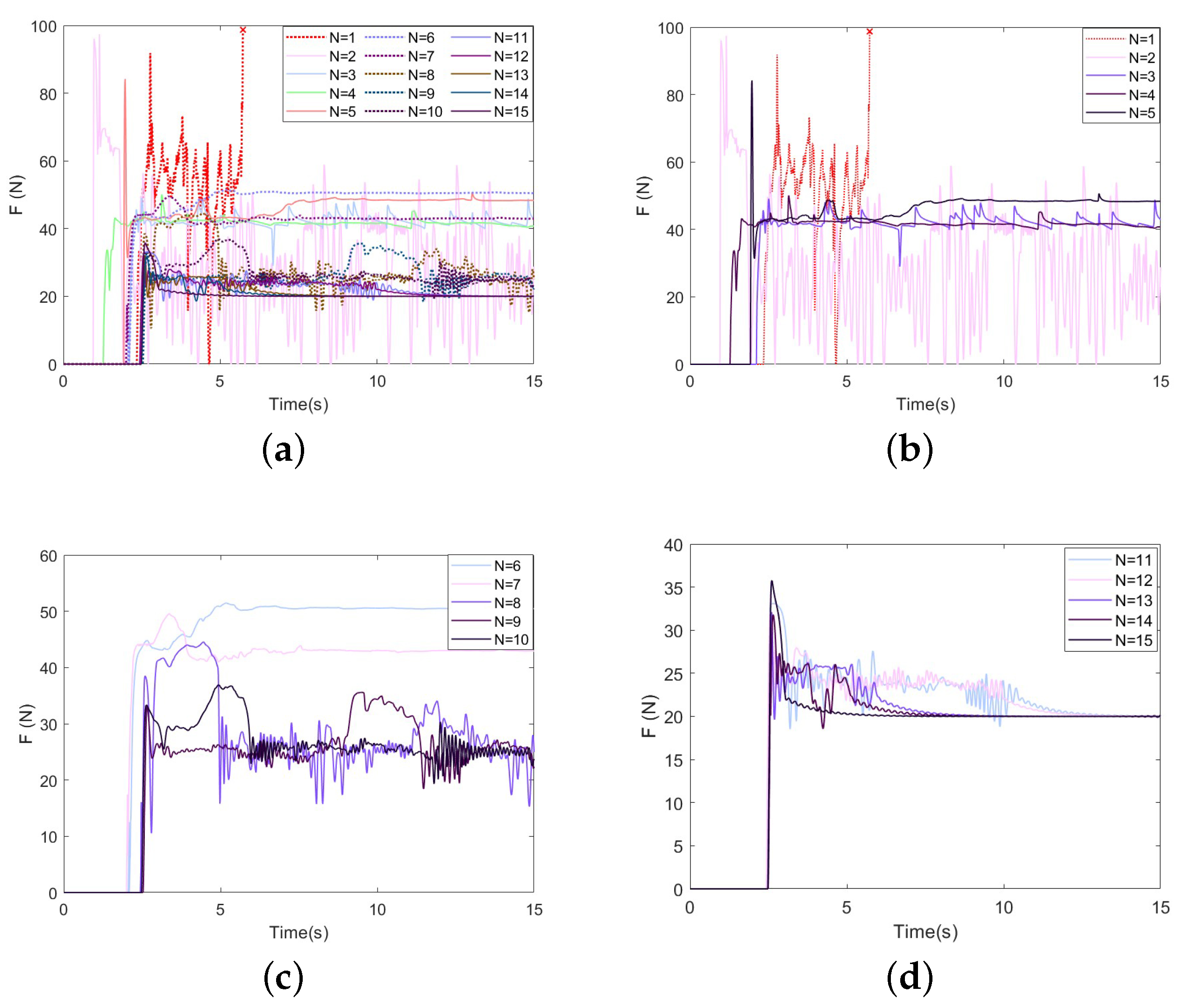
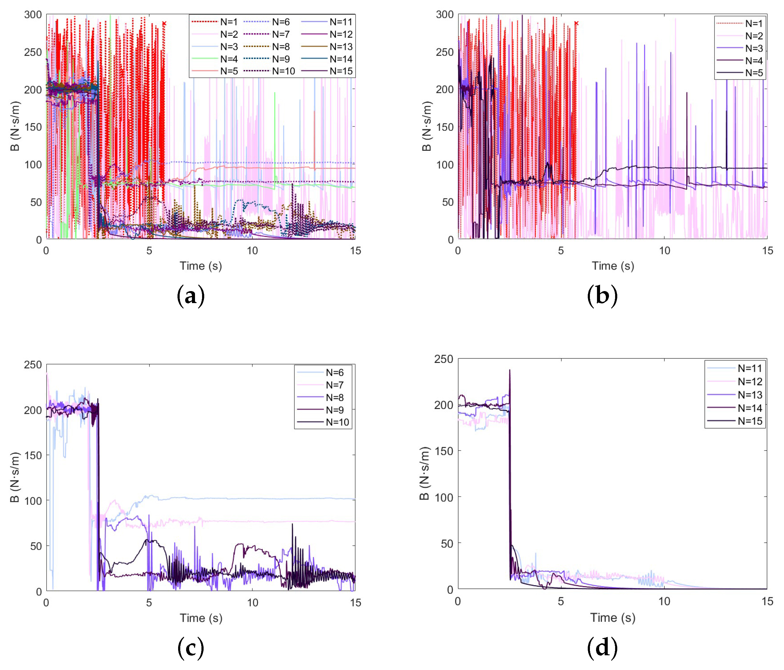
The GP-DDPG algorithm without initial policy is used for simulations, and the other conditions remain unchanged. Figure 9 and Figure 10 show the experimental results. It can be seen from the figures that, due to the lack of prior experience, the contact force exceeds 100 N in the first training, and the task fails. After a period of training, the algorithm can still converge and reach at , but it is delayed by about 33% compared with the algorithm with initial policy. It only converges to the locally optimal solution.
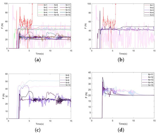
Figure 9.
Force-tracking performance of GP-DDPG without initial policy: (a) The change in force in 1∼15 learnings; (b) N = 1∼5; (c) N = 5∼10; (d) N = 10∼15.

Figure 10.
Damping variation performance of GP-DDPG without initial policy: (a) The change in damping in 1∼15 learnings; (b) N = 1∼5; (c) N = 5∼10; (d) N = 10∼15.
4.1.2. Performance of Intelligent Admittance Control in an Uncertain Environment
In the following experiments, the rough initial position of the environment is known, and the speed and acceleration of the actual environmental change is not zero, which is the environmental uncertainty for which the controller has to compensate. The simulation results of our algorithm are compared with the constant admittance control and the classical adaptive admittance control shown in Equation (15).
Firstly, the force-tracking performance under the variable stiffness plane is evaluated. The task is the same as in Section 4.1.1, and the variable stiffness plane is . The environmental stiffness is set to
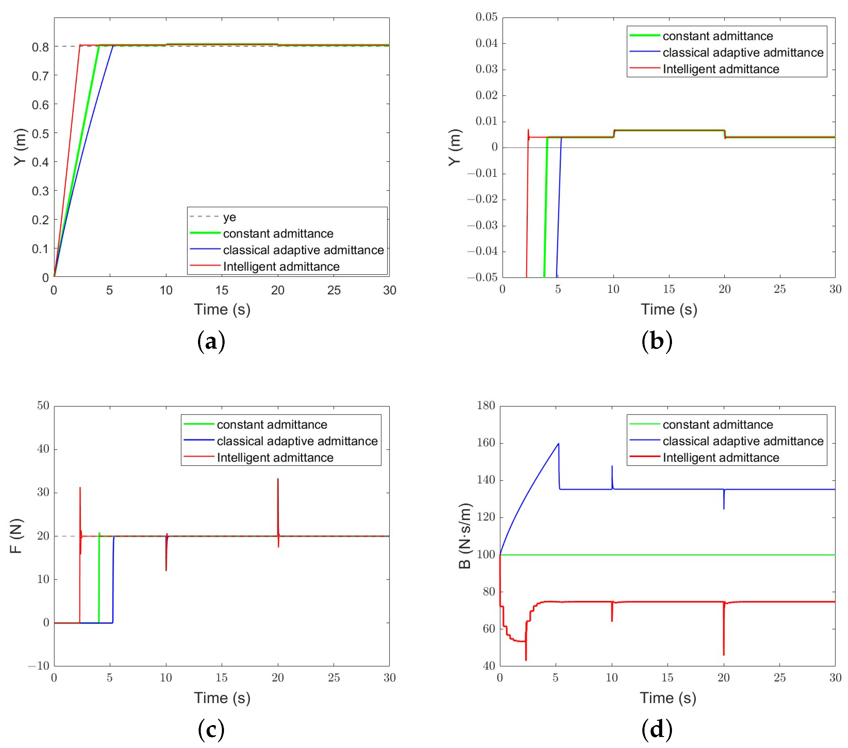
The constant admittance control parameter is set to , ; for , there is . Figure 11 illustrates the trajectory-tracking and force-tracking performance of the three methods. It can be seen from the figure that all three methods can achieve force tracking. Among them, the intelligent admittance controller contacts the environment within 3–4 s, which is faster than the other two methods. When the environmental stiffness changes, the abrupt force causes a short overshoot and then recovers quickly.
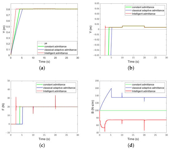
Figure 11.
The performance of each algorithm under the variable stiffness plane: (a) Position-tracking performance; (b) position-tracking error; (c) force-tracking performance; (d) evolution of the damping parameter.
From Figure 11, it can be seen that the evolution trend of the damping parameter B of classical adaptive admittance control and intelligent admittance control is obviously different. Overall, the damping parameter of intelligent admittance control is significantly smaller than that of classical adaptive admittance control, because it takes into account the energy consumption term a. When the robot is not in contact with the environment, the damping of classical adaptive admittance control increases with time, which reduces the acceleration of the robot and, thus, alleviates the unknown collision. When the contact force appears, it becomes smaller immediately. In the learning process, intelligent admittance control takes into account the speed error , force error , and energy consumption . When the robot is not in contact with the environment, the damping parameter is reduced so that the robot can reach the environment quickly. However, small damping also leads to an increase in overshoot.
Next, the performance in a complex environment (the speed and acceleration of the environment are not constant) is evaluated. In this paper, a complex surface that changes according to exponential sine curves is designed.
The contact surface changes with time as follows:
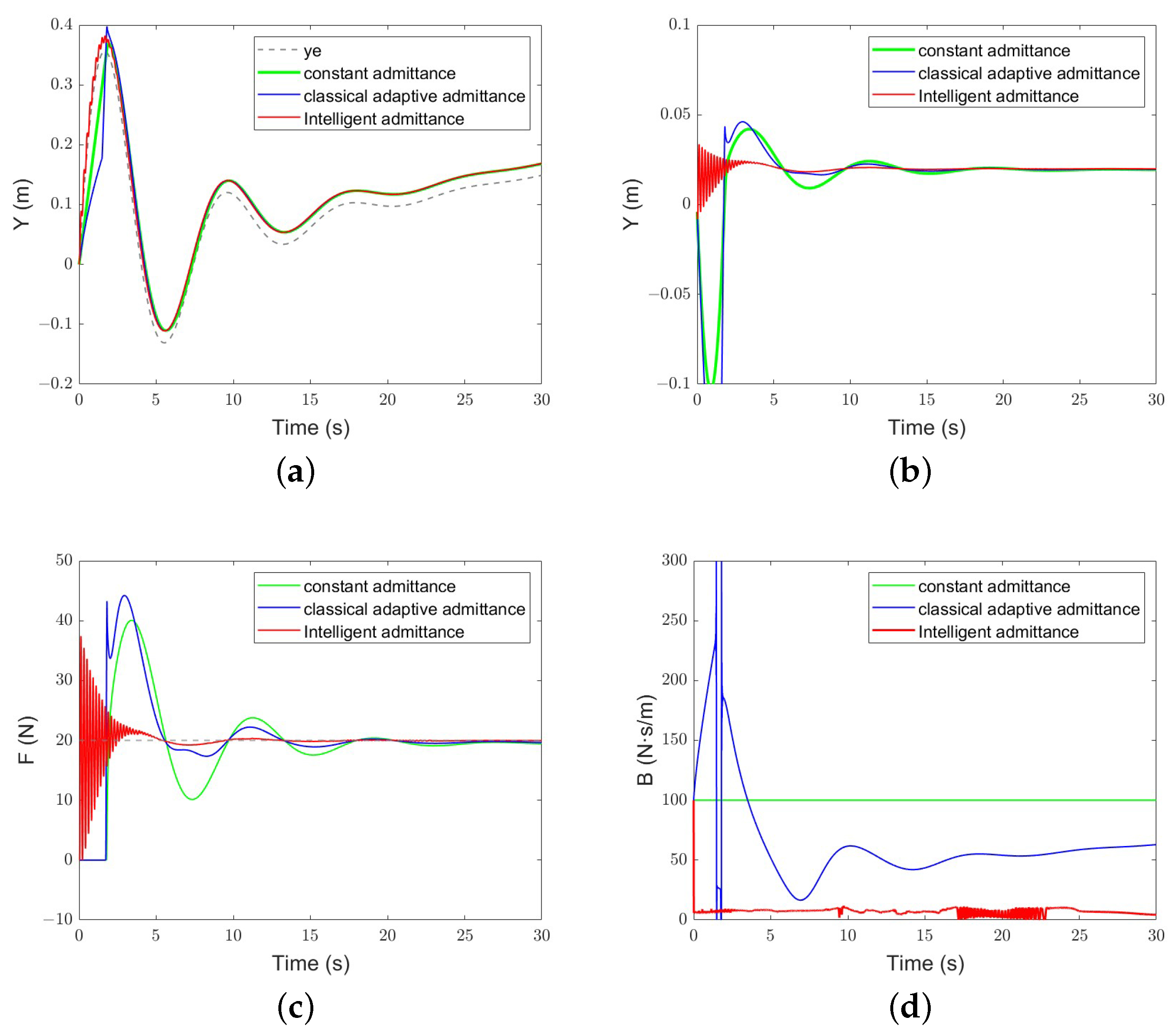
The initial position of the origin of the robot end is set to ; for , there is and , and the other conditions remain unchanged. Compared with the sinusoidal surface, the change in the class-exponential sinusoidal surface is irregular, so it can better reflect the robustness of the algorithm. Figure 12 illustrates the performance of the algorithm. The constant admittance control cannot converge. The classical adaptive admittance control converges after a period of adjustment. After training, the robustness of the intelligent admittance control is obviously better than the former, and the response time is faster.
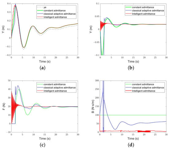
Figure 12.
The performance of each algorithm under the complex environment: (a) Position-tracking performance; (b) position-tracking error; (c) force-tracking performance; (d) evolution of the damping parameter.
From Figure 12, it can be seen that the evolution trend of the damping parameter B of classical adaptive admittance control is similar to that in the variable stiffness simulation. It is worth noting that, when the system has not yet reached the steady state, our algorithm obtains a smaller damping value, which makes the robot reach and adapt to the environment faster, but also causes high-frequency oscillation, which may have a negative impact on the stability of the system in the application. In order to reduce the high-frequency oscillation of the system, the weight parameters in the reward can be adjusted appropriately to reduce the consideration of energy consumption and reduce the speed of the decrease of the damping parameter value.
Based on the results of the three simulations, the algorithm we designed has the best performance. The constant admittance control cannot guarantee the force tracking in all environmental stiffnesses, while the adaptive admittance algorithm has poor tracking effect in low-stiffness conditions, and there is a large jitter in the face of complex surfaces. Our algorithm can stably control the force error at the micron level, and the resistance to environmental stiffness changes is better than the first two.
4.2. Experimental Results
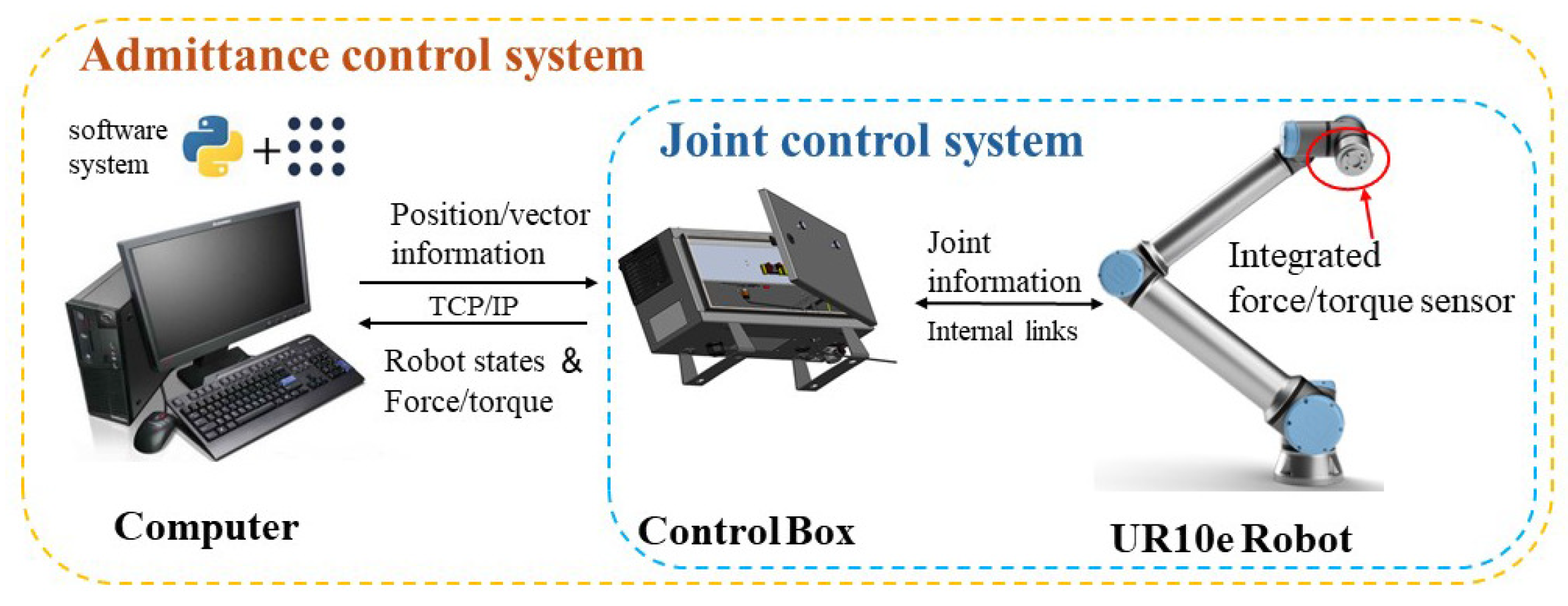
To further verify the proposed algorithm, the UR10e manipulator is used as the experimental object for experimental verification. Figure 13 shows the environment of this experiment. UR10e integrates the force/torque sensor. The sensor has a Z direction measurement range of 100 N and an accuracy of 5.5 N (in the experiment, the read force/torque data are filtered). Using python, a software system based on ROS is built in the Linux environment. The computer communicates with the manipulator control box through the TCP/IP protocol, sends motion instructions, and obtains the real-time status of the manipulator with a ommunication frequency of 250 HZ.

Figure 13.
Hardware configuration of the experiment.
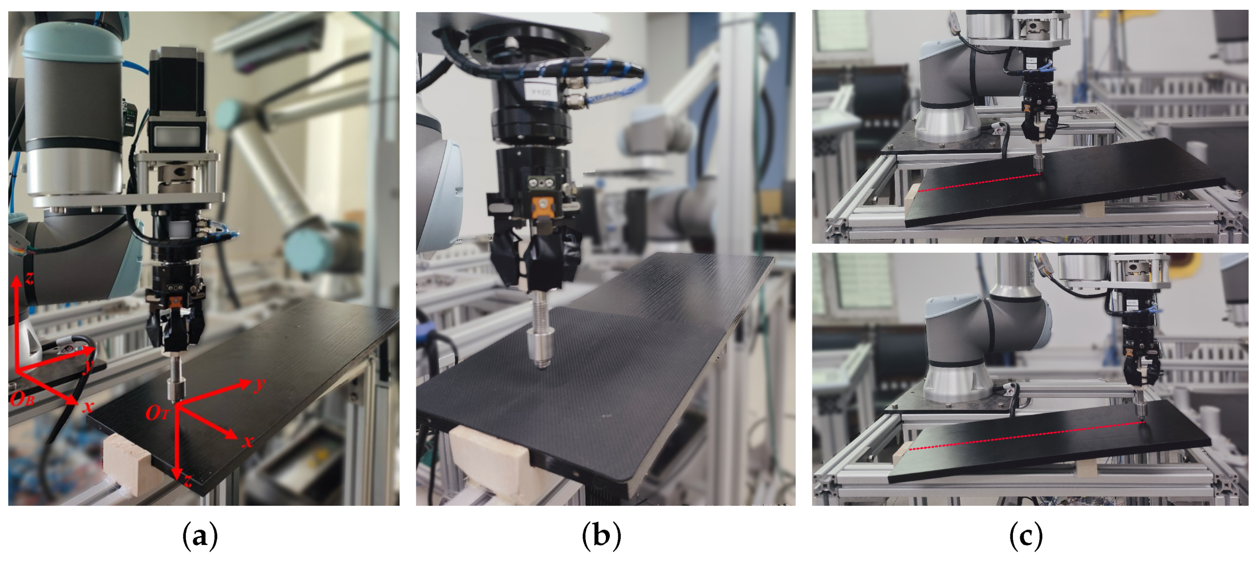
The experimental scene is shown in Figure 14. This paper shows three experiments, in which the environment is a slope. In the first experiment, the slope of the slope was steeper, and in the second experiment, the slope of the slope was gentler. The third experiment changed the environmental characteristics and covered the soft rubber material at one end of the slope. Combined with the accuracy of the force sensor and the force drift when the end is suspended, the allowable force error is set to ±2.5 N in this paper. The experiments compare three algorithms of constant admittance, classical adaptive admittance, and intelligent variable admittance, which are the same as the algorithms compared in the simulation.
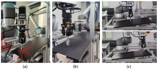
Figure 14.
The real-world experiment. (a) Experimental installation. The tool coordinate system is , the base coordinate system is , and the mapping between the two can be calculated by the robot kinematics. At this time, the specific location of the slope is unknown to the control system. (b) Different environments in the third experiment. (c) Experimental process. The red dotted line represents the trajectory of the robot.
The desired force of 20 N is set on the Z axis. The constant-admittance control parameter is set to , . , , and are the same as the simulation. For , there is and . The characteristic is unknown.
In the steep slope experiment, the end-effector is hovered above a hard slope, that is, the position of the base coordinate system Z = 0.115 m, and moves forward along the y-axis on a fixed slope.
The results are shown in Figure 15, Figure 16 and Figure 17. All three methods have a certain compliance effect. Under the constant admittance control, the end-effector of the robot collides with the slope after about 23 s and generates overshoot. After a period of adjustment, it still cannot track the required force, and the force error always stays at about 7.5 N.

Figure 15.
Constant-admittance control steep slope tracking performance: (a) force-tracking performance; (b) position-tracking performance; (c) evolution of the damping parameter.

Figure 16.
Classical adaptive-admittance steep control slope tracking performance: (a) force-tracking performance; (b) position-tracking performance; (c) evolution of the damping parameter.

Figure 17.
Intelligent-admittance control steep slope tracking performance: (a) force-tracking performance; (b) position-tracking performance; (c) evolution of the damping parameter.
Under the classical adaptive admittance control, the end-effector of the robot collides with the inclined plane after about 13 s. After adjustment, it slowly converges to the expected force. The evolution trend of the damping parameter is the same as that in the simulation. When the environment is not contacted, the damping parameter increases continuously and decreases rapidly after contacting the environment. However, due to the measurement error in the equipment and environment and the influence of noise, the evolution of the damping parameter also has large jitter.
Under the control of intelligent admittance, the robot touches the slope and generates overshoots after about 10 s, and the desired force can be tracked smoothly in about 80 s. On average, the damping parameter of intelligent admittance control is still smaller than that of classical adaptive-admittance control. Compared with the latter, the damping change of intelligent admittance control is more obvious, which is also the reason why it reaches the environment faster and realizes force tracking earlier.
The overshoot may cause damage to the robot. When other conditions remain unchanged, the overshoot will increase with the increase in the expected contact force because the force error will affect the change in the motion state. Collision is unavoidable. In industrial assembly applications, when the expected force is small (which is also the purpose of force control), the overshoots of the three algorithms shown in the experiments are not enough to cause harm to the workpiece and robot in the assembly of high-strength metal materials, which is acceptable.
In the gentle slope experiment, the position of the base coordinate system Z = 0.113 m, and it moves forward along the y-axis on a fixed slope.
The results are shown in Figure 18, Figure 19 and Figure 20. Under the constant-admittance control, the robot collides with the slope after about 16.7 s and generates overshoot. After a period of adjustment, it still cannot track the required force, and the force error always stays at about 4.8 N. Under the classical adaptive-admittance control, the robot collides with the inclined plane after about 20.5 s, and then is in a state of overshoot for some time. After adjustment, it converges to the expected force at 104.9 s. For the intelligent-admittance control, the robot touches the slope and generates overshoots after about 10.4 s, and the desired force can be tracked smoothly in about 63.9 s. It can be seen that there is no prominent change in the force-tracking performance of each algorithm.

Figure 18.
Constant-admittance control gentle slope tracking performance: (a) force-tracking performance; (b) position-tracking performance; (c) evolution of the damping parameter.

Figure 19.
Classical adaptive-admittance control gentle slope tracking performance: (a) force-tracking performance; (b) position-tracking performance; (c) evolution of the damping parameter.

Figure 20.
Intelligent-admittance control gentle slope tracking performance: (a) force-tracking performance; (b) position-tracking performance; (c) evolution of the damping parameter.
It is worth noting that all algorithms are slower to reach the environment because the initial position of the robot is farther away from the environment. In addition, the force overshoot is reduced compared to the force overshoot of the steep slope, and the convergence speed of the variable-admittance algorithm is improved.
In the third experiment, the characteristics and location of the environment changed, and the setting of the slope was the same as in the first experiment. The position of the base coordinate system Z = 0.115 m, and we set the Z axis force to 5 N.
The results are shown in Figure 21, Figure 22 and Figure 23. Under the constant-admittance control, the robot is in contact with the environment at about 12.2 s, while classical adaptive-admittance control is about 24.2 s and intelligent-admittance control is about 8.6 s. When passing through the rubber material, none of the three can stably track the expected force, which may be caused by the overly soft material. However, it is gratifying that, after a small amount of overshoot caused by the switching of materials, all three algorithms can track the desired force. Among them, the constant-admittance control needs to experience 22.2 s, classical adaptive-admittance control needs to experience 18.9 s, and intelligent-admittance control needs to experience 12.1 s.

Figure 21.
Constant-admittance control for different environments’ characteristic tracking performance: (a) force-tracking performance; (b) position-tracking performance; (c) evolution of the damping parameter.

Figure 22.
Classical adaptive-admittance control for different environments’ characteristic tracking performance: (a) force-tracking performance; (b) position-tracking performance; (c) evolution of the damping parameter.

Figure 23.
Intelligent-admittance control for different environments’ characteristic tracking performance: (a) force-tracking performance; (b) position-tracking performance; (c) evolution of the damping parameter.
The experimental results further prove the feasibility of the intelligent control algorithm designed in this paper. The overshoots of the three algorithms of constant admittance, classical adaptive admittance, and intelligent variable admittance are within the allowable range. The adjustment time of intelligent variable-admittance is better than that of classical adaptive-admittance control, and its advantages rise with the dramatic changes in the environment. When the experimental environment is a steep slope, it is improved by about 44%. When the environment is a gentle slope, it is improved by 39%. When there is a flexible material in the environment as a buffer for collision and the expected force is smaller, it is improved by 35.9%.
5. Discussion and Conclusions
To improve the adaptability and safety of a robot working in an uncertain environment, an intelligent-admittance control algorithm based on DDPG combined with classical control is proposed. Simulations and experiments are set up to verify the performance of the algorithm. The algorithm is based on reinforcement learning, combines the GP model with DDPG, and can converge to the expected value by using fewer than 15 instances of learning in the simulation.
To verify the superiority of the algorithm, which combines classical control theory and reinforcement learning theory, the control experiments of the algorithm without initial policy and the algorithm with initial policy are set up. From the simulation results, the convergence speed of the algorithm with initial policy is 33% higher than that of the algorithm without initial policy. And the algorithm without initial policy has a task failure due to excessive contact force in the early stage of training. The algorithm with initial policy avoids this failure well, thus improving security.
To verify the performance of the algorithm in an uncertain environment, the simulation of a variable-stiffness environment and complex environment are set up, and the results are compared with those of constant-admittance control and adaptive-admittance control. In the variable-stiffness environment experiment, all three algorithms can adapt to environmental changes and track the desired force. Among them, the speed of the intelligent-admittance algorithm to contact the environment is about 48% higher than that of other algorithms. In the complex environment experiment, assuming that the force control accuracy is ±0.2 N, the constant admittance control cannot track the contact force. The adaptive admittance control can track the contact force at about 26 s, while the intelligent admittance control can track the contact force at about 12 s and the speed is increased by about 53.84%.
Simulation represents an ideal world. To further verify the performance of the proposed algorithm, three experiments with a slope as the environment were set up, and the experiment was completed with a 6-DOF manipulator. In the slope surface experiments, the constant-admittance control cannot track the desired force when the expected force is large. The adaptive-admittance control can track the contact force, but its convergence speed is not as fast as that of intelligent admittance control, and this gap will become more obvious with the change in environment. In the experiments in this paper, the performance of intelligent admittance control can be improved by 44% compared with the traditional adaptive admittance control. The experimental results are highly similar to the simulation results, which can prove the effectiveness of the simulation.
The disadvantage is that, in the simulations and experiments, this paper only focuses on the tracking performance of the algorithm in a single dimension, and verifies the algorithm under a simple model. In the future, we plan to apply it to specific assembly tasks, consider more environmental interference, and conduct research on dual-robot collaborative assembly tasks.
Author Contributions
Conceptualization, B.J. and X.H.; methodology, X.H.; software, P.R. and Y.L.; validation, B.J., X.H., P.R., and Y.L.; formal analysis, X.H.; investigation, B.J.; resources, G.L. and B.J.; data curation, Y.L.; writing—original draft preparation, X.H. and L.L.; writing—review and editing, S.D., B.J., X.H., and L.L.; visualization, L.L. and S.D.; supervision, G.L. and B.J.; funding acquisition, B.J. All authors have read and agreed to the published version of the manuscript.
Funding
This research was funded by Equipment Development Department of People’s Republic of China Central Military Commission grant number [62502010223] and Department of Science and Technology of Jilin Province Key R&D Project grant number [20230201097GX].
Institutional Review Board Statement
Not applicable.
Informed Consent Statement
Not applicable.
Data Availability Statement
The original contributions presented in the study are included in the article; further inquiries can be directed to the corresponding author.
Acknowledgments
The authors sincerely appreciate the support provided by their institutions.
Conflicts of Interest
Authors Gongping Liu and Peipei Ren were employed by the company Avic Xi’an Aircraft Industry Group Co., Ltd., author Shilin Duan was employed by the company Sichuan Huachuan Industry Co., Ltd.. The remaining authors declare that the research was conducted in the absence of any commercial or financial relationships that could be construed as a potential conflict of interest.
References
- Kim, Y.; Yoon, W.C. Generating Task-Oriented Interactions of Service Robots. IEEE Trans. Syst. Man Cybern. Syst. 2014, 44, 981–994. [Google Scholar] [CrossRef]
- Kang, T.; Yi, J.-B.; Song, D.; Yi, S.-J. High-Speed Autonomous Robotic Assembly Using In-Hand Manipulation and Re-Grasping. Appl. Sci. 2021, 11, 37. [Google Scholar] [CrossRef]
- Hélio, O.; Cortesão, R. Impedance control architecture for robotic-assisted mold polishing based on human demonstration. IEEE Trans. Ind. Electron. 2022, 69, 3822–3830. [Google Scholar] [CrossRef]
- Qiao, H.; Wang, M.; Su, J.; Jia, S.; Li, R. The Concept of “Attractive Region in Environment” and its Application in High-Precision Tasks with Low-Precision Systems. IEEE ASME Trans. Mechatronics 2015, 20, 2311–2327. [Google Scholar] [CrossRef]
- Siciliano, B.; Villani, L. Robot Force Control; Springer: New York, NY, USA, 1999. [Google Scholar]
- Zhu, R.; Yang, Q.; Song, J.; Yang, S.; Liu, Y.; Mao, Q. Research and Improvement on Active Compliance Control of Hydraulic Quadruped Robot. Int. J. Control Autom. Syst. 2021, 19, 1931–1943. [Google Scholar] [CrossRef]
- Craig, J.J.; Raibert, M.H. A systematic method of hybrid position/force control of a manipulator. In Proceedings of the COMPSAC 79, Proceedings, Computer Software and The IEEE Computer Society’s Third International Applications Conference, Chicago, IL, USA, 6–8 November 1979; pp. 446–451. [Google Scholar] [CrossRef]
- Hogan, N. Impedance Control: An Approach to Manipulation. In Proceedings of the 1984 American Control Conference, San Diego, CA, USA, 6–8 June 1984; pp. 304–313. [Google Scholar] [CrossRef]
- Hu, H.; Cao, J. Adaptive variable impedance control of dual-arm robots for slabstone installation. ISA Trans. 2022, 128, 397–408. [Google Scholar] [CrossRef]
- Liu, X.; Li, Z.; Pan, Y. Preliminary Evaluation of Composite Learning Tracking Control on 7-DoF Collaborative Robots. IFAC-PapersOnLine 2021, 54, 470–475. [Google Scholar] [CrossRef]
- Grafakos, S.; Dimeas, F.; Aspragathos, N. Variable admittance control in pHRI using EMG-based arm muscles co-activation. In Proceedings of the 2016 IEEE International Conference on Systems, Man, and Cybernetics (SMC), Budapest, Hungary, 9–12 October 2016; pp. 001900–001905. [Google Scholar] [CrossRef]
- Wai, H.; Hlaing, W.; Myo, A.; Sin, T. Variable admittance controller for physical human robot interaction. In Proceedings of the IECON 2017—43rd Annual Conference of the IEEE Industrial Electronics Society, Beijing, China, 29 October–1 November 2017; pp. 2929–2934. [Google Scholar] [CrossRef]
- Duan, J.; Gan, Y.; Chen, M.; Dai, X. Adaptive variable impedance control for dynamic contact force tracking in uncertain environment. Robot. Auton. Syst. 2018, 102, 54–65. [Google Scholar] [CrossRef]
- Yamane, K. Admittance Control with Unknown Location of Interaction. IEEE Robot. Autom. Lett. 2021, 6, 4079–4086. [Google Scholar] [CrossRef]
- Abu-Dakka, F.J.; Rozo, L.; Caldwell, D.G. Force-based variable impedance learning for robotic manipulation. In Proceedings of the 2018 IEEE-RAS 18th International Conference on Humanoid Robots (Humanoids), Beijing, China, 6–9 November 2018; pp. 1–9. [Google Scholar] [CrossRef]
- Takahashi, C.D.; Scheidt, R.A.; Reinkensmeyer, D.J. Impedance control and internal model formation when reaching in a randomly varying dynamical environment. J. Neurophysiol. 2001, 86, 1047–1051. [Google Scholar] [CrossRef]
- Tsuji, T.; Tanaka, Y. Bio-mimetic impedance control of robotic manipulator for dynamic contact tasks. Robot. Auton. Syst. 2008, 56, 306–316. [Google Scholar] [CrossRef]
- Lee, K.; Buss, M. Force Tracking Impedance Control with Variable Target Stiffness. IFAC Proc. Vol. 2008, 41, 6751–6756. [Google Scholar] [CrossRef]
- Kronander, K.; Billard, A. Learning Compliant Manipulation through Kinesthetic and Tactile Human-Robot Interaction. IEEE Trans. Haptics 2014, 7, 367–380. [Google Scholar] [CrossRef] [PubMed]
- Lai, G.; Liu, Z.; Zhang, Y.; Chen, C.L.P. Adaptive Position/Attitude Tracking Control of Aerial Robot with Unknown Inertial Matrix Based on a New Robust Neural Identifier. IEEE Trans. Neural Netw. Learn. Syst. 2016, 27, 18–31. [Google Scholar] [CrossRef]
- Yang, C.; Peng, G.; Cheng, L.; Na, J.; Li, Z. Force Sensorless Admittance Control for Teleoperation of Uncertain Robot Manipulator Using Neural Networks. IEEE Trans. Syst. Man Cybern. Syst. 2021, 51, 3282–3292. [Google Scholar] [CrossRef]
- He, W.; Dong, Y.; Sun, C. Adaptive Neural Impedance Control of a Robotic Manipulator with Input Saturation. IEEE Trans. Syst. Man Cybern. Syst. 2016, 46, 334–344. [Google Scholar] [CrossRef]
- Liu, Y.-J.; Tong, S.; Chen, C.L.P.; Li, D.-J. Neural Controller Design-Based Adaptive Control for Nonlinear MIMO Systems with Unknown Hysteresis Inputs. IEEE Trans. Cybern. 2016, 46, 9–19. [Google Scholar] [CrossRef]
- Zhang, X.; Sun, L.; Kuang, Z.; Tomizuka, M. Learning Variable Impedance Control via Inverse Reinforcement Learning for Force-Related Tasks. IEEE Robot. Autom. Lett. 2021, 6, 2225–2232. [Google Scholar] [CrossRef]
- Noppeney, V.; Boaventura, T.; Siqueira, A. Task-space impedance control of a parallel Delta robot using dual quaternions and a neural network. J. Braz. Soc. Mech. Sci. Eng. 2021, 43, 440. [Google Scholar] [CrossRef]
- Hamedani, M.H.; Sadeghian, H.; Zekri, M.; Sheikholeslam, F.; Keshmiri, M. Intelligent Impedance Control using Wavelet Neural Network for dynamic contact force tracking in unknown varying environments. Control Eng. Pract. 2021, 113, 104840. [Google Scholar] [CrossRef]
- Xu, Z.; Li, X.; Wu, H.; Zhou, X. Dynamic neural networks based adaptive optimal impedance control for redundant manipulators under physical constraints. Neurocomputing 2022, 471, 149–160. [Google Scholar] [CrossRef]
- Li, G.; Yu, J.; Chen, X. Adaptive Fuzzy Neural Network Command Filtered Impedance Control of Constrained Robotic Manipulators with Disturbance Observer. IEEE Trans. Neural Netw. Learn. Syst. 2023, 34, 5171–5180. [Google Scholar] [CrossRef] [PubMed]
- Prabhu, S.M.; Garg, D.P. Fuzzy-logic-based Reinforcement Learning of Admittance Control for Automated Robotic Manufacturing. Eng. Appl. Artif. Intell. 1998, 11, 7–23. [Google Scholar] [CrossRef]
- Roveda, L.; Maskani, J.; Franceschi, P.; Abdi, A.; Braghin, F.; Tosatti, J.M.; Pedrocchi, N. Model-Based Reinforcement Learning Variable Impedance Control for Human-Robot Collaboration. J. Intell. Robot. Syst. 2020, 100, 417–433. [Google Scholar] [CrossRef]
- Li, M.; Wen, Y.; Gao, X.; Si, J.; Huang, H. Toward Expedited Impedance Tuning of a Robotic Prosthesis for Personalized Gait Assistance by Reinforcement Learning Control. IEEE Trans. Robot. 2022, 38, 407–420. [Google Scholar] [CrossRef]
- Peng, G.; Chen, C.L.P.; Yang, C. Neural Networks Enhanced Optimal Admittance Control of Robot–Environment Interaction Using Reinforcement Learning. IEEE Trans. Neural. Netw. Learn. Syst. 2022, 33, 4551–4561. [Google Scholar] [CrossRef]
- Khader, S.A.; Yin, H.; Falco, P.; Kragic, D. Stability-Guaranteed Reinforcement Learning for Contact-Rich Manipulation. IEEE Robot. Autom. Lett. 2021, 6, 1–8. [Google Scholar] [CrossRef]
- Li, C.; Zhang, Z.; Xia, G.; Xie, X.; Zhu, Q. Efficient Force Control Learning System for Industrial Robots Based on Variable Impedance Control. Sensors 2018, 18, 2539. [Google Scholar] [CrossRef]
- Ding, Y.; Zhao, J.; Min, X. Impedance control and parameter optimization of surface polishing robot based on reinforcement learning. Proc. Inst. Mech. Eng. Part J. Eng. Manuf. 2023, 237, 216–228. [Google Scholar] [CrossRef]
- He, W.; Mu, X.; Zhang, L.; Zou, Y. Modeling and trajectory tracking control for flapping-wing micro aerial vehicles. IEEE/CAA J. Autom. Sin. 2021, 8, 148–156. [Google Scholar] [CrossRef]
- He, W.; Wang, T.; He, X.; Yang, L.-J.; Kaynak, O. Dynamical Modeling and Boundary Vibration Control of a Rigid-Flexible Wing System. IEEE ASME Trans. Mechatronics 2020, 25, 2711–2721. [Google Scholar] [CrossRef]
- Lillicrap, T.P.; Hunt, J.J.; Pritzel, A.; Heess, N.; Erez, T.; Tassa, Y.; Silver, D.; Wierstra, D. Continuous control with deep reinforcement learning. arXiv 2015, arXiv:1509.02971. [Google Scholar] [CrossRef]
- Cheng, R.; Orosz, G.; Murray, R.M.; Burdick, J.W. End-to-End Safe Reinforcement Learning through Barrier Functions for Safety-Critical Continuous Control Tasks. In Proceedings of the AAAI Conference on Artificial Intelligence, Honolulu, HI, USA, 27 January–1 February 2019; pp. 3387–3395. [Google Scholar] [CrossRef]
- Berkenkamp, F.; Turchetta, M.; Schoellig, A.P.; Krause, A. Safe Model-based Reinforcement Learning with Stability Guarantees. In Advances in Neural Information Processing Systems; Curran Associates, Inc.: Red Hook, NY, USA, 2017. [Google Scholar] [CrossRef]
- Kronander, K.; Billard, A. Stability Considerations for Variable Impedance Control. IEEE Trans. Robot. 2016, 32, 1298–1305. [Google Scholar] [CrossRef]
Disclaimer/Publisher’s Note: The statements, opinions and data contained in all publications are solely those of the individual author(s) and contributor(s) and not of MDPI and/or the editor(s). MDPI and/or the editor(s) disclaim responsibility for any injury to people or property resulting from any ideas, methods, instructions or products referred to in the content. |
© 2024 by the authors. Licensee MDPI, Basel, Switzerland. This article is an open access article distributed under the terms and conditions of the Creative Commons Attribution (CC BY) license (https://creativecommons.org/licenses/by/4.0/).


