Abstract
To address the control challenges of an aerial manipulator arm (AMA) mounted on a drone under conditions of model inaccuracy and strong disturbances, this paper proposes a hierarchical control architecture. In the upper-level control, Bézier curves are first used to generate smooth and continuous desired trajectory points, and the theory of singular trajectory lines along with a Radial Basis Function Neural Network (RBFNN) is introduced to construct a highly accurate multi-configuration inverse kinematic solver. This solver not only effectively avoids singular solutions but also enhances its precision online through data-driven methods, ensuring the accurate calculation of joint angles. The lower-level control focuses on optimizing the dynamic model of the manipulator. Using a Model Predictive Control (MPC) strategy, the dynamic behavior of the manipulator is predicted, and a rolling optimization process is executed to solve for the optimal control sequence. To enhance system robustness, an RBFNN is specifically introduced to compensate for external disturbances, ensuring that the manipulator maintains stable performance in dynamic environments and computes the optimal control commands. Physical prototype testing results show that this control strategy achieves a root mean square (RMS) error of 0.035, demonstrating the adaptability and disturbance rejection capabilities of the proposed method.
1. Introduction
With the rapid advancement of technology, the use of drones equipped with robotic arms for aerial tasks is rapidly penetrating various industries, particularly the power industry [1]. Traditional manual methods for repairing broken wires, maintaining clamps, tightening bolts, and removing obstacles in power transmission lines are not only inefficient but also high-risk [2,3]. This necessitates the search for innovative solutions. The emergence of drones with robotic arms offers a timely, efficient, and safe alternative.
The aerial robotic arm system integrates advanced rotary-wing drones, intelligent line-walking devices, and multifunctional robotic arms. It can precisely track target trajectories in complex and dynamic aerial environments, ensuring the smooth completion of various maintenance tasks [4,5]. The core competitiveness of this system lies in the precise control of the AMA. Only with such precision can the accuracy and efficiency of operations be ensured. Therefore, in-depth research and optimization of AMA control strategies have become urgent technical challenges that need to be addressed.
Scholars, both domestically and internationally, have conducted extensive research on the control issues of aerial manipulators. Ding et al. proposed an impedance control method, decomposing the aerial manipulator system into three control loops—lateral, longitudinal, and manipulator—each with its own control strategy, achieving significant results. However, research on the dynamic control of aerial manipulator systems remains insufficient [6]. Zain Anwar Ali designed an adaptive control scheme combining regulation, pole placement, and tracking (RST) control, which is suitable for the nonlinear control of underactuated quadrotors. This scheme optimizes system performance through the MIT rule, enabling the drone equipped with a camera and gripper to perform tasks in hard-to-reach locations, with simulations and experiments verifying the superior performance of the designed controller [7].
Zhang’s research focused on the modeling and control of aerial manipulators. He proposed a dynamic model considering the dynamic coupling effects of the manipulator on the drone and, based on this model, designed a disturbance-compensating robust H∞ controller to ensure flight stability during manipulator operations. Experimental results confirmed the effectiveness of this control strategy. For tasks under strong wind disturbances [8]. Zhang also designed an acceleration feedback-enhanced robust H∞ controller, effectively suppressing wind disturbances and ensuring stable hovering and high-precision operation of the aerial manipulator [9].
Zhong’s work focused on solving the complex kinematics, dynamics, and control design issues of aerial manipulator systems. By using spherical camera geometric dynamics and image feature passive error equations, combined with task-priority control schemes, he achieved excellent performance in visual servo control, with outdoor experimental results validating the practicality and effectiveness of autonomous aerial manipulation [10]. Tlatelpa-Osorio proposed a dual-loop control strategy, compensating for the mutual influences between the drone and manipulator separately, ensuring independent control of the drone and manipulator and maintaining stability even under external disturbances [11].
Khanmirza’s contribution was the introduction of an aerial manipulator with flexible arms and a new trajectory planning and control algorithm to minimize adverse effects such as vibration caused by flexible components. Facing increased underactuation and control complexity under flexible conditions, the research derived dynamic equations using the Lagrange formula and addressed constraints corresponding to link flexibility [12]. Cai proposed a fault-tolerant control (FTC) scheme for aerial manipulators, ensuring transient and steady-state tracking performance even in the event of actuator failures. By designing a novel performance function (NPF) and adaptive non-singular terminal sliding mode control, along with an extended state observer, the scheme effectively handled complex coupling effects and external disturbances, ensuring system stability [13].
Luo’s research focused on the problem of picking up parcels from mobile robots by aerial manipulators in the shortest time. Using discrete mechanics and complementary constraint framework, he optimized trajectory planning, ensuring the best total travel time within dynamic constraints and improving the efficiency of time-optimal switching trajectory planning [14]. Qiu utilized a strategy combining neural networks and reinforcement learning for tracking control and trajectory optimization, which significantly enhanced control accuracy and outperformed traditional PD control [15,16].
Despite significant achievements in various fields of research, AMA control technology still faces severe challenges, with two core issues worth focusing on:
- (1)
- Difficulty in precise model construction: The deep coupling and mutual interference between the AMA, the drone, and the walking mechanism make it extremely complex to accurately depict their kinematic and dynamic characteristics, directly affecting the accuracy of operations.
- (2)
- Difficulty in controlling external disturbances: During aerial operations, the AMA is significantly affected by wind and the drone’s own disturbances, exacerbating the instability and uncertainty of the control system.
Based on this, to address the two key issues currently facing the AMA, this paper proposes an innovative hierarchical control system. This system ensures the accuracy of the inverse kinematic solver by integrating singular trajectory theory with an RBFNN and enhances the stability and disturbance rejection capabilities of the AMA through a combined control approach of MPC and RBFNN. The control system is divided into two main modules: the upper layer focuses on path planning and inverse kinematics optimization, while the lower layer is dedicated to dynamic optimization and disturbance rejection.
In the upper-layer control, Bézier curves are used to generate coherent and smooth reference trajectory points, ensuring the accuracy and fluidity of AMA movements. To overcome model accuracy limitations and avoid singular postures, the STL theory and RBFNN are introduced to construct highly accurate inverse kinematic solvers for four different configurations. This multi-module inverse kinematic solver effectively avoids singularities and enhances the solver’s accuracy through data-driven methods, ensuring precise joint angle calculations.
The lower-layer control focuses on optimizing the dynamic model of the robotic arm. By employing MPC strategies, the dynamic behavior of the robotic arm is predicted and modeled, and a rolling optimization process is performed to obtain the optimal control sequence. To enhance system robustness, an RBFNN is introduced to compensate for external disturbances, ensuring that the robotic arm maintains stable performance in dynamically changing environments, thus calculating the optimal control commands.
Therefore, the hierarchical control architecture proposed in this study not only significantly improves the trajectory tracking accuracy of drone-operated robotic arms but also enhances the system’s adaptability and disturbance rejection capabilities, providing a solid technical foundation for the efficient execution of future drone payload missions.
The subsequent chapters of this paper are organized as follows: Section 2 constructs the kinematic and dynamic models of the aerial manipulator; Section 3 details the design principles and implementation methods of the aerial manipulator control system based on hierarchical control theory; Section 4 evaluates the robustness and stability of the proposed control strategy through simulation experiments; Section 5 demonstrates the setup of the physical verification platform and its experimental verification results, visually validating the theoretical analysis and design; and finally, Section 6 summarizes the research findings.
2. Mathematical Model
2.1. Kinematic Model of the AMA
Most modern manipulators adhere to Pieper’s criterion, where three adjacent joint axes either intersect at a single point or are mutually parallel [17]. The first three degrees of freedom determine the position of the end-effector, while the last three degrees of freedom determine its orientation [18], as illustrated in Figure 1 and Table 1.
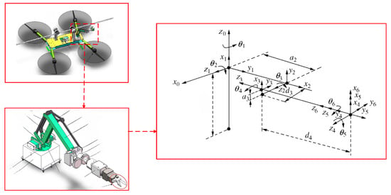
Figure 1.
Coordinate system of a 6-DOF aerial manipulator arm.

Table 1.
Explanation of the kinematic and dynamic mathematical symbols for the AMA.
The workspace of an aerial manipulator arm, defined as the set of all possible positions that the end-effector can reach, is a critical factor in the study of robotic operations and holds significant importance for the effectiveness of these operations [19]. Therefore, this paper focuses on the positioning mechanism of a six-DOF robot, fixing the orientation mechanism to simplify it into the AMA.
The aerial manipulator arm uses the MDH method to establish the link coordinate system [20], thereby determining the parameters of the manipulator’s links, as shown in Table 2.

Table 2.
Physical parameters of the AMA.
Based on the link coordinate system and structural parameters of the aerial manipulator arm, the transformation matrix between adjacent link coordinate systems can be derived as follows:
where .
By multiplying the transformation matrices of each link, the pose matrix of the end-effector of the manipulator arm is obtained.
where ,
, ,
, ,
, , ,
,
represents the position vector of the end reference point relative to the floating coordinate system, and represents the orientation transformation matrix of the end reference point relative to the floating coordinate system.
This paper investigates the position trajectory tracking of the AMA. According to the above equations, the position control depends only on the first three joint angles . To simplify calculations, the subsequent joint angles are fixed at .
The Jacobian matrix of the AMA is obtained by computing the partial derivatives of the end-effector position with respect to the joint angles [21]. This can be represented as :
From Equation (3), the determinant of the Jacobian matrix for the aerial manipulator can be expressed as
2.2. Dynamic Model of AMA
The dynamics of the AMA are modeled using the Lagrange method, defining the set of joint position variables AMA as the generalized coordinates [22]. The Lagrange function of the AMA in the generalized coordinates is defined as follows:
where and are the total kinetic and potential energy of the AMA, respectively; is the generalized velocity of the joint; is the mass of the joint; is the length of the link; is the distance from the centroid of the joint to the joint axis; and is the gravitational acceleration.
The Lagrange equation can be expressed as [23]
In the dynamic model, are the state variables, and is the control variable.
The partial derivatives of the joint angle, joint angular velocity, and angular acceleration are further computed as follows:
Substituting Equation (6) into Equation (7), the dynamic equation of the AMA is obtained as
3. Control Design
Facing the challenges of insufficient model accuracy and strong disturbances in the AMA, this study proposes an innovative hierarchical control architecture aimed at achieving high-precision trajectory tracking control. This architecture consists of an upper-layer path planning and a lower-layer dynamic control, as shown in Figure 2.
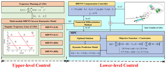
Figure 2.
Block diagram of the trajectory tracking control system based on the hierarchical control method.
In the upper control system, Bézier curves are used as the path planning tool to generate continuous and smooth trajectories for the inverse kinematics model. To overcome the limitations of model accuracy and avoid issues caused by singular postures, we introduce singular trajectory line theory and RBFNN. By constructing highly accurate inverse kinematic solvers for four different configurations and integrating a data-driven learning mechanism, we enhance the real-time accuracy of the inverse kinematic solver, ensuring precise calculation of joint angles.
At the lower control level, we employ numerical differentiation techniques to accurately derive joint angular velocities and accelerations as input parameters for the dynamic model. By implementing the MPC strategy, we can predict the dynamic behavior of the manipulator and execute a rolling optimization algorithm to obtain the optimal control sequence. To enhance system robustness, especially against external disturbances, we incorporate RBFNN for compensation, ensuring the stable performance of the manipulator in dynamically changing environments and thereby computing the optimal control commands.
Through this hierarchical control method, we have significantly improved the trajectory tracking accuracy of the AMA while greatly enhancing its stability and anti-interference capability.
3.1. Trajectory Planning of the AMA
To achieve optimal dynamic performance, the trajectory planning for the AMA mounted on a drone must adhere to the following key principles [24,25]:
- (1)
- Suppression of joint impacts: The planning process should fully consider the forces on each joint to avoid excessive instantaneous impact forces due to improper planning. This helps extend the service life of the manipulator arm and enhances operational safety.
- (2)
- Smoothness of joint velocity and acceleration: The planned trajectory should ensure that the changes in joint velocity and acceleration are gradual and continuous, avoiding any abrupt or extreme points to achieve smoother motion performance and reduce unnecessary energy consumption.
- (3)
- To minimize impact forces during the AMA’s operation, the desired trajectory is often planned in the form of a cycloid. However, given the unique advantages of Bézier curves—including their intuitive control characteristics, strong expressive ability, and the ease of generating complex and smooth curves—they have become the preferred method for manipulator trajectory planning in the industry.
Bézier curves can accurately depict the required smooth trajectory through a set of control points and specific mathematical formulas, ensuring that the AMA can flexibly adapt to changing working environments while maintaining high precision in control [26].
where is the order of the Bézier curve, represents the interpolation points at , and is the control point. By selecting values for within , an arbitrary number of interpolation points can be generated between and . This paper uses a cubic Bézier curve, which is expressed as
3.2. A Multi-Module Inverse Kinematic Model Based on Singular Trajectory Lines and RBF Neural Networks
3.2.1. Derivation of Singular Trajectory
As shown in Equation (4), the Jacobian matrix varies with changes in the arm joints. However, when ( or ), the matrix is non-invertible, meaning does not exist. Consequently, the matrix is considered “singular” or “degenerate”. The corresponding arm position is referred to as a singular configuration, and the point in the operational space is known as a singular point. When a manipulator reaches a singular configuration, it physically loses one or more degrees of freedom [27,28]. Mathematically, this is determined by checking whether the determinant of the Jacobian matrix is zero. Points where the determinant of the Jacobian matrix is zero are identified as singular points of the manipulator.
From the determinant of the Jacobian matrix for the AMA, it is clear that the singular points of the manipulator are independent of and are only related to parameters and . Set:
When the determinant is , there are two possible scenarios.
- (1)
- Boundary singular configuration
That is, or 1.6178 rad.
When , the manipulator is in a fully extended state; when , the manipulator is in a fully retracted state. Therefore, the singular points of the manipulator appear on the boundary of the workspace, and the line segments formed by connecting these singular points are called singular trajectory lines. As shown in Figure 3, there are two horizontal singular trajectory lines when β = 0.
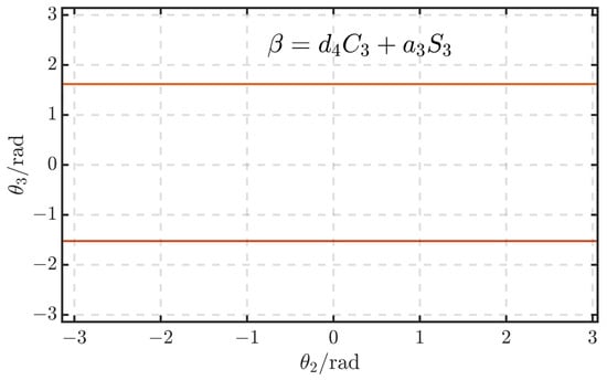
Figure 3.
Singular trajectories of β = 0.
- (2)
- Internal singular configurationwhere , .
Internal singular configurations occur within the workspace when two or more joint axes coincide, resulting in a loss of degrees of freedom. As shown in Figure 4, the singular trajectory line for γ = 0. By merging the singular trajectory lines for β = 0 and γ = 0, the singular trajectory lines in the joint space of the AMA are formed, as illustrated in Figure 5. These singular trajectory lines divide the joint space into nine unequal regions.
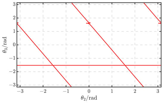
Figure 4.
Singular trajectories of γ = 0.
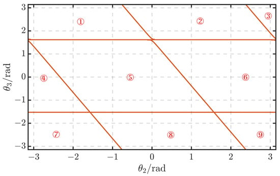
Figure 5.
The singular trajectory of the AMA in the joint space.
The singular trajectory lines for β = 0 and γ = 0 are combined to form the singular trajectory lines in the joint space of the AMA, as shown in Figure 5. It can be observed that these singular trajectory lines divide the joint space into nine unequal regions.
3.2.2. Partitioning of the Joint Space Based on STL for Single Inverse Solutions
Since the AMA must pass through a singular point when transitioning from one inverse kinematic solution to another, each inverse kinematic solution is strictly separated by singular trajectory lines. This means that within a closed singular trajectory line, only a single inverse solution exists [25]. As shown in Figure 5, region ⑤ is a closed parallelogram enclosed by singular trajectory lines, so the joint space in region ⑤ contains only a single inverse solution. Because the joint variation range of and is periodic with a period of 2π, the remaining eight regions can be combined into a complete closed parallelogram region through or , as shown in Table 2. Therefore, the joint space of the AMA can be divided into four parallelogram joint spaces, each containing only a single inverse solution. By randomly selecting coordinate points within these four parallelogram regions to obtain the joint variables and , the link structure of each region can be plotted using the forward kinematics function with the help of the Robotics Toolbox to determine the type of inverse solution, as shown in Figure 6 and Table 3.
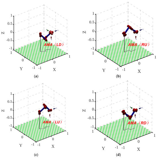
Figure 6.
Inverse solution of AMA structure diagram: (a) The left elbow-down configuration of AMA. (b) The right elbow-up configuration of AMA. (c) The left elbow-up configuration of AMA. (d) The right elbow-down configuration of AMA.

Table 3.
Distribution of AMA inverse solutions based on singular trajectories.
In summary, the inverse kinematic solutions of the AMA can be categorized into four types: left_elbow-up (LU), left_elbow-down (LD), right_elbow-up (RU), and right_elbow-down (RD).
The distribution of the single inverse solution joint subspaces based on singular trajectory lines in the entire joint space and their corresponding configurations are shown in Figure 6.
3.2.3. Multi-Module RBFNN Kinematic Model
The RBFNN has been proven to approximate any continuous function to any desired degree of accuracy [29]. In an RBF neural network, the first layer is the input layer, with the number of nodes equal to the dimensionality of the input; the second layer is the hidden layer, with the number of nodes determined by the complexity of the problem, using radial basis functions as the basis functions; the third layer is the output layer, with the number of nodes equal to the dimensionality of the output data [30]. The structure of the RBFNN is shown in Figure 7.
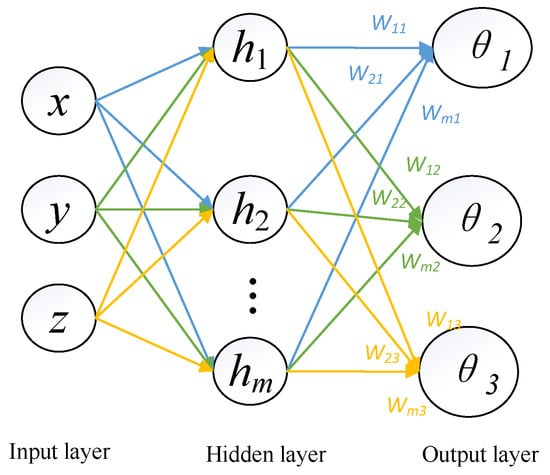
Figure 7.
Multiple input, multiple output RBNN structure diagram.
Let the radial basis vector be and be the output of the neuron in the hidden layer.
where is the coordinate vector of the center point of the Gaussian basis function in the hidden layer, and is the width of the Gaussian basis function for the neuron in the hidden layer.
The output of the RBFNN is
where is the weight of the RBFNN.
Given a desired target trajectory to track , the performance index function of the RBFNN is
The output weights , node widths , and center vector parameters are iteratively optimized using the gradient descent method [31].
The four joint regions containing only a single inverse solution (LU, LD, RU, RD), obtained from the singular trajectory lines, are mapped to the same workspace using a mapping method from joint space to workspace, and the selection of the joint variable . This results in four sets of training samples with the same workspace but different corresponding inverse solution regions. Each neural network module is responsible for learning one set of training samples and predicting the same set of test samples. This approach extends from the traditional single neural network, which can only predict one type of inverse solution, to a multi-module neural network structure capable of outputting four different types of inverse solutions.
3.3. Model Predictive Control System for the AMA
The dynamic equations of the AMA describe the input-output relationship of the manipulator system and can thus be used as a predictive model for MPC. However, Equation (8) is a time-varying second-order non-homogeneous differential equation and cannot be directly used as a predictive model [32,33]. Therefore, it needs to be linearized and discretized to obtain a model suitable for predictive control.
Based on the AMA dynamics Equation (8), the relationship between joint acceleration and system input, as well as state variables, is given by
The state variable of the AMA system is , and the control input is . By performing a Taylor expansion at the time instant , setting the sampling period to , and transforming to the incremental model () followed by discretization, the prediction model is obtained as
where , , , .
From Equation (18), given the current system state , the predicted state of the system for steps ahead is
Therefore, the trajectory tracking prediction equation for the future state of the manipulator is derived as follows:
where , , , .
In Equation (20), is the prediction horizon, is the control horizon, , represents the prediction of the future state of the system, is the system input matrix for the prediction, and is the constant increment. is the prediction state matrix, and is the prediction control matrix.
To minimize the error of the AMA during trajectory tracking, the following objective function can be selected [34]:
where the symbol represents the predicted state of the system at future time step , given the information available at the current time step , and and represent the weight coefficient matrices for each part.
The objective function defined in Equation (20) aims to minimize the tracking error of AMA during trajectory tracking. This function comprises two parts: the first part is the weighted squared sum of the deviation between the predicted state and the reference state , while the second part is the weighted squared sum of the control input variation . The objective function seeks to balance trajectory tracking accuracy with control input smoothness [35].
The trajectory tracking problem of the AMA can be transformed into solving the above optimization problem at each time step while satisfying the constraint conditions [36]:
This optimization problem is a standard Quadratic Programming (QP) problem. In this paper, the interior-point method is utilized, employing numerical optimization techniques to iteratively solve for the optimal control input that minimizes the objective function.
Based on the current state of the AMA and the control input from the previous time step, the above optimization problem can be solved to obtain the optimal control increment [37]. Thus, the current optimal control input is
3.4. Compensation Control System Based on RBFNN
In the MPC-based AMA control system, the inaccuracy of the dynamic model and external disturbances may affect the system’s robustness. Therefore, it is necessary to incorporate external disturbances into the control model:
At the same time, the dynamic model has assumptions and discrepancies from the actual nominal model. Assuming the accurate nominal model of the manipulator is , , and , the relationship between the nominal model and the dynamic mathematical model established in this paper is as follows [38]:
Therefore, by combining Equations (24) and (25) with the assumed nominal model, the following dynamic equation is obtained, which considers both the complete dynamic model of the AMA and external disturbances:
In the AMA control system, the nominal model is used. If is known, the control law can be set as follows:
where .
Substituting Equation (27) into Equation (24), the error system is obtained as follows:
where is the desired angle command. , .
The control objective is to design a stable, robust controller based on the nominal model. However, in practical engineering, is usually unknown. Therefore, the RBF neural network is used to estimate .
where represents the optimal network weights of the RBF neural network in the compensation system, and represents the Gaussian functions in the hidden layer of the compensation system.
The training of primarily involves pre-training using the state variables and the control input from the MPC control system as the training set. Subsequently, real-time parameter updates are performed using the gradient descent method as the system operates.
4. Validation Test Results
This section validates the effectiveness of the proposed control method through numerical simulations. These simulations were conducted in a specific computational environment and are detailed as follows:
- Computational platform: The numerical simulations were performed on a desktop computer equipped with an Intel Core i7-9700K CPU @ 3.60 GHz and 32 GB RAM;
- Operating system: Windows 10 Professional;
- Programming language and software: All numerical computations and simulations were carried out in the MATLAB 2021a environment, utilizing MATLAB’s Model Predictive Control Toolbox and Neural Network Toolbox for MPC and RBFNN-related computations;
- Simulation settings: The simulation time was set to 5 s with a time step of 0.01 s to ensure the accuracy and stability of the results.
4.1. Mapping of Single Inverse Solution Space and Proof of Multiple Solutions for AMA
In the joint subspaces LU, LD, RU, and RD, which are strictly divided by singular trajectory lines and contain only a single inverse solution, coordinate points are collected using a loop program to obtain the range of values for and for each inverse solution configuration. Through forward kinematics, the nonlinear mapping from joint space to workspace is achieved.
As shown in Figure 8, when , all four joint subspaces can be mapped to four identical spherical position spaces. This position space represents the complete workspace of the AMA.
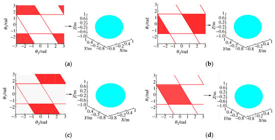
Figure 8.
Nonlinear mapping of joint space to working space: (a) left elbow down; (b) left elbow up; (c) right elbow up; (d) right elbow down.
Based on the above analysis, the four joint regions LD, LU, RD, and RU can all obtain the complete workspace of the AMA through forward kinematics. This verifies the correctness of the single inverse solution space regions divided by singular trajectory lines and also proves the multiplicity of inverse kinematic solutions for the same workspace.
4.2. Training of the Multi-Module RBF Neural Network
This study constructs the joint spaces of LD, LU, RD, and RU based on the singular trajectory line theory, aiming to achieve precise learning and simulation of complex motion patterns through offline training and online optimization of a multi-module RBFNN. To ensure the model’s generalization ability and robustness, we divided the dataset into three parts: 70% for training to capture core features, 15% for validation to adjust hyperparameters and prevent overfitting, and the remaining 15% for final testing to examine the model’s practical performance.
The training results are intuitively displayed in Figure 9 and Table 4, clearly reflecting the convergence process and performance metrics of each neural network module. Notably, after sufficient iterative training, all four RBFNNs demonstrated excellent learning efficiency, successfully meeting the predetermined testing standards.
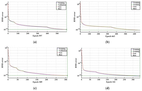
Figure 9.
Training performance curve of the multi-module neural network: (a) RBF neural network (LD); (b) RBF neural network (LU); (c) RBF neural network (RD). (d) RBF neural network (RU).

Table 4.
The RMS error of the multi-module neural network test.
Specifically, the RBFNN (LD) achieved an RMS error of 8.4958 × 10¹¹ after 597 iterations; the RBFNN (LU) achieved an RMS error of 5.1462 × 10¹¹ after 663 iterations; the RBFNN (RD) reached an RMS error of 7.1697 × 10¹¹ after only 309 iterations; and the RBFNN (RU) achieved an RMS error as low as 6.7838 × 10¹¹ after 341 iterations. These results not only demonstrate the powerful capability of RBFNN in handling complex mapping tasks in joint space but also highlight the crucial role of singular trajectory line theory in guiding network structure design and training strategy selection.
4.3. AMA Trajectory Tracking Simulation Test
This section presents the AMA trajectory tracking test of the hierarchical control algorithm designed in this study. A smooth trajectory was planned using a Bézier curve with a runtime of 5 s to verify the algorithm’s performance. Figure 10 visually compares the output results of MPC and RBFNN compensation control.
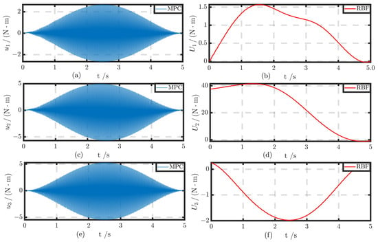
Figure 10.
Comparison of outputs between MPC and RBFNN control: (a) control output of under MPC control; (b) control output of under RBFNN control; (c) control output of under MPC control; (d) control output of under RBFNN control; (e) control output of under MPC control; (f) control output of under RBFNN control.
The output of the MPC control strategy demonstrates its centrally symmetric distribution characteristics, with amplitude variations over time. This reflects the MPC system’s ability to ensure control stability and accuracy by effectively responding to dynamic environmental changes through continuous feedback adjustments. The MPC system meticulously adjusts the control signals to maintain stable and accurate system responses. On the other hand, RBFNN compensation control compensates for model inaccuracies and external disturbances through a feedforward approach.
As shown in Figure 11 and Table 5, during the trajectory tracking experiment, the MPC system initially exhibited fluctuations and steady-state errors, with the RMS error reaching 0.03488. However, when combined with RBF compensation control, the system quickly tracked the preset trajectory, consistently demonstrating high levels of stability and control precision. The MPC + RBFNN combination showcased excellent control capabilities, rapidly correcting deviations and maintaining stable performance throughout the operation.
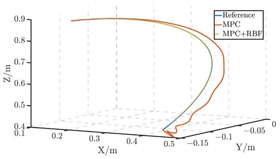
Figure 11.
The AMA trajectory tracking simulation curves.

Table 5.
The RMS error of trajectory tracking control.
In the joint angle tracking comparison analysis shown in Figure 12, it is evident that when using only the MPC strategy, the three joint angles , , and exhibit persistent steady-state errors. Specifically, the RMS errors for these joint angles reached 0.025439 radians, 0.0078973 radians, and 0.022519 radians, respectively, indicating that the tracking accuracy of the system is somewhat limited under MPC control.
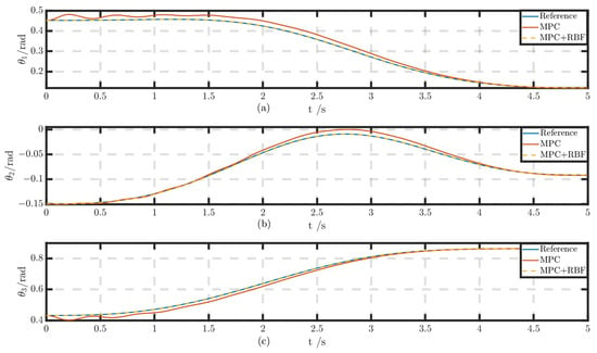
Figure 12.
The AMA joint tracking curves: (a) angle tracking curve of ; (b) angle tracking curve of ; (c) angle tracking curve of .
However, when the MPC control strategy is combined with RBFNN compensation control, the tracking performance of the three joint angles significantly improves. In this MPC + RBF composite control mode, the RMS errors of , , and are effectively reduced to 0.0062576 radians, 0.0038244 radians, and 0.0062192 radians, respectively. This result clearly demonstrates the role of RBFNN compensation control in enhancing tracking accuracy and reducing steady-state errors, enabling the system to more accurately and stably follow the desired joint angle changes.
In the joint angular velocity tracking comparison experiment shown in Figure 13 and Table 6, it can be observed that the angular velocities of and fluctuate significantly within the first 2.5 s but then tend to stabilize; however, the angular velocity of shows substantial fluctuations in the first second, followed by reduced yet persistent oscillations. When only using the MPC control, the tracking performance for the angular velocities of the three joints is suboptimal, with RMS errors reaching 0.020767 rad/s, 0.12112 rad/s, and 0.03774 rad/s, respectively.
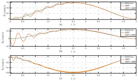
Figure 13.
The AMA joint velocity tracking curves: (a) speed tracking curve of ; (b) speed tracking curve of ; (c) speed tracking curve of .

Table 6.
The RMS error of joint angle and joint angular velocity tracking.
However, with the introduction of the MPC + RBF composite control system, the tracking performance of the angular velocities of , , and has significantly improved. The system can quickly respond and maintain the stability of joint angular velocities, exhibiting excellent performance not only in smooth transitions throughout the tracking process but also in quantitative evaluations. Specifically, under MPC + RBF control, the RMS errors of the angular velocities of the three joints were effectively reduced to 0.0099134 rad/s, 0.019756 rad/s, and 0.021185 rad/s. This indicates that the addition of the RBF compensation controller greatly enhances tracking accuracy and stability, effectively suppressing angular velocity fluctuations and ensuring superior system performance in dynamic environments.
In the AMA trajectory tracking simulation test, we found that the combination of MPC and RBFNN demonstrated exceptional stability and precise tracking capabilities. Compared to using MPC alone, the MPC + RBF system showed significantly better performance in joint angles, joint angular velocities, and overall trajectory tracking. By integrating the high-precision feedback control of MPC with the feedforward advantages of RBF compensation control, the trajectory tracking performance of AMA was notably enhanced. This improvement is reflected not only in higher tracking accuracy but also in the system’s increased adaptability to external disturbances and effective compensation for model errors, ensuring robust operation and precise task execution of AMA in complex dynamic environments.
The method proposed in this paper is compared with the methods from the literature in terms of trajectory tracking accuracy, as shown in Table 7. The method in Reference [9] performs well with an RMS error of 0.02488 m, which is the smallest among the compared methods from the literature but still larger than the method proposed in this paper. The method in Reference [11] has an RMS error of 0.0289 m, slightly worse than that of Reference [9]. The method in Reference [14] performs the worst, with an RMS error of 0.0358 m, indicating a larger tracking error. The RMS error of the method proposed in this paper is significantly lower than those of the other methods, at only 0.0096157 m, demonstrating that the method proposed in this paper achieves the highest accuracy and the smallest error in trajectory tracking.

Table 7.
Comparison of RMS errors in trajectory tracking between this method and methods from different references.
As seen in Table 6, the method proposed in this paper performs excellently in trajectory tracking, with an RMS error far lower than that of the other methods from the literature, indicating that the proposed method offers higher accuracy and better performance in trajectory tracking control.
5. Experimental Details and Results
5.1. Physical Prototype Introduction
The aerial robot, comprising a flight platform and an AMA, is dedicated to the efficient removal of debris from power transmission lines. Considering the robot’s unique structural characteristics and the need for separate control systems, we have meticulously designed four critical electrical control system modules, as shown in Figure 14: the power management and distribution system, the flight control system, the operational environment perception system, and the AMA control system. These modules work in close collaboration to achieve efficient system operation and precise control.
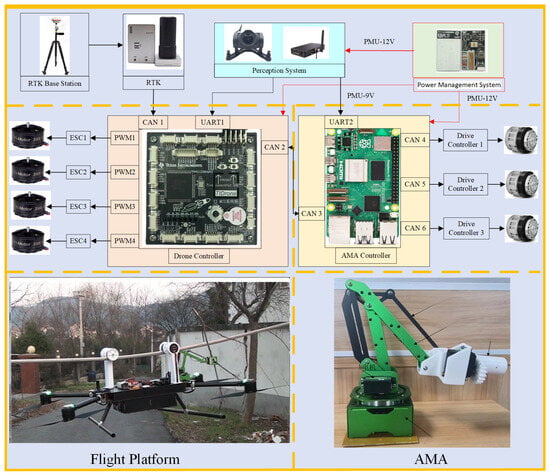
Figure 14.
Electrical flow diagram of the physical prototype.
- (1)
- Flight control system: At the heart of the flight control system is a controller board based on the STM32H743, integrated with an Inertial Measurement Unit (IMU) to ensure flight stability. The system connects to an RTK system via a CAN bus interface, enabling high-precision positioning. It features four PWM outputs that directly control the four rotor motors, ensuring precise maneuverability of the flight platform. Additionally, the flight control system interfaces with the operational environment perception system and the AMA control system via UART and CAN interfaces, facilitating information sharing and collaborative operation among modules.
- (2)
- AMA control system: The AMA control system is focused on performing debris removal tasks, with an advanced Raspberry Pi 5b as the core control unit mounted on an expansion board. This system features three CAN interfaces, establishing communication with the three joint motors of the manipulator arm, allowing for precise control of the manipulator’s movements and effective manipulation of the end-effector tools to efficiently remove targeted debris.
5.2. The AMA Trajectory Tracking Operation Experiment
In this chapter, to validate the practical effectiveness of the proposed algorithm, we conducted an AMA trajectory tracking experiment on a real flight platform using a physical testbed. The objective was to remove foreign objects, such as kites or branches, from power lines. During the experiment, the flight platform first navigated to the power line location and securely attached itself to the line. Subsequently, the AMA performed the cleaning task. Throughout this process, the AMA had to overcome the effects of wind disturbances and the strong coupling with the flight platform itself. As seen in the experiment Figure 15, the AMA successfully removed the obstacles, and the entire operation was smooth without noticeable shaking or oscillations.
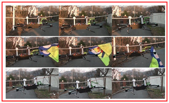
Figure 15.
Physical animation of AMA trajectory tracking during obstacle-clearing operation.
Figure 16 and Figure 17 illustrate the AMA’s tracking curves throughout the trajectory tracking process, including the tracking curves along three axes in three-dimensional space. From these graphs, it is clear that the AMA maintained high stability and accuracy during the power line obstacle removal process. Table 8 presents the RMS error data from this experiment. The overall RMS error for the AMA trajectory tracking was 0.035448 m, while the RMS errors along the three axes were 0.016853 m, 0.021278 m, and 0.022799 m, respectively. These values clearly indicate that our control algorithm achieved a high level of accuracy, fully meeting the expected control requirements and confirming the feasibility and effectiveness of the method in practical applications.
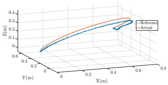
Figure 16.
The AMA trajectory tracking experimental test curves.
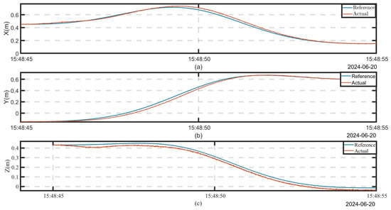
Figure 17.
Trajectory tracking curves for X-axis, Y-axis, and Z-axis: (a) Tracking curve on the X-axis. (b) Tracking curve on the Y-axis. (c) Tracking curve on the Y-axis.

Table 8.
The RMS error of AMA trajectory tracking.
6. Conclusions
The innovation of this paper lies in the introduction of a hierarchical control structure for an AMA to address issues of model accuracy insufficiency and strong disturbances, thereby achieving precise trajectory tracking control. The specific innovations include the following:
Upper-level control: Utilizing Bézier curves to generate smooth and continuous desired trajectory points, ensuring accurate and fluid movement of the manipulator. To overcome model accuracy limitations and avoid singular poses, the STL theory and the RBFNN are introduced, constructing a high-precision inverse kinematic RBFNN solver suitable for four different configurations. This multi-module inverse kinematic solver not only avoids singular solutions but also enhances the solver’s accuracy online through a data-driven approach, ensuring precise calculation of joint angles.
Lower-level control: Focusing on optimizing the manipulator’s dynamic model. The MPC strategy is employed to predict and simulate the dynamic behavior of the manipulator, followed by solving the optimal control sequence through a rolling optimization process. To enhance system robustness, RBFNN is specifically introduced to compensate for external disturbances, ensuring that the manipulator maintains stable performance even in dynamically changing environments, thus computing optimal control commands. In the physical experiments conducted, the RMS error of AMA’s trajectory tracking was 0.035448 m, demonstrating high trajectory tracking accuracy and stability performance.
In summary, the proposed hierarchical control architecture not only significantly improves the trajectory tracking accuracy of the manipulator mounted on the UAV but also enhances the system’s adaptability and anti-interference capabilities, providing a solid technical foundation for the efficient execution of future UAV payload missions.
Author Contributions
Conceptualization, H.Z., Z.Y. and Y.Y.; methodology, H.Z., Z.Y. and Y.Y.; software, Z.Y., Y.Y., H.Z., N.X. and L.L.; validation, Z.Y. and Y.Y.; formal analysis, Z.Y., Y.Y., H.Z. and J.W.; investigation, Z.Y. and Y.Y.; resources, Z.Y. and Y.Y.; data curation, Y.Y., H.Z., Z.Y. and J.W.; writing—original draft preparation, Z.Y. and Y.Y.; writing—review and editing, Z.Y., Y.Y., H.Z., L.L., J.W. and J.H.; visualization, H.Z., Z.Y. and Y.Y.; supervision, H.Z. and Z.Y.; project administration, Z.Y.; funding acquisition, Z.Y. All authors have read and agreed to the published version of the manuscript.
Funding
This work was supported by Funding for Outstanding Doctoral Dissertation in NUAA (project approval no. BCXJ23-05), by “Guangxi Power Grid Company’s 2023 Science and Technology Innovation Project under Grant GXKJXM20230169”, and by “the Guizhou Provincial Science and Technology Projects under Grant Guizhou-Sci-Co-Supp[2020]2Y044”.
Data Availability Statement
Data are contained within the article.
Conflicts of Interest
Author Haoze Zhuo was employed by the company Electric Power Research Institute of Guangxi Power Grid Co., Ltd., The remaining authors declare that the research was conducted in the absence of any commercial or financial relationships that could be construed as a potential conflict of interest.
References
- Chen, Y.; Wu, Y.; Zhang, Z.; Miao, Z.; Zhong, H.; Zhang, H.; Wang, Y. Image-Based Visual Servoing of Unmanned Aerial Manipulators for Tracking and Grasping a Moving Target. IEEE Trans. Ind. Inform. 2023, 19, 8889–8899. [Google Scholar] [CrossRef]
- Han, X.; Liu, X.; Wu, G.; Song, X.; Cui, L. Research on Additive Manufacturing Path Planning of a Six-Degree-of-Freedom Manipulator. Actuator 2024, 13, 249. [Google Scholar] [CrossRef]
- Paul, H.; Miyazaki, R.; Kominami, T.; Ladig, R.; Shimonomura, K. A Versatile Aerial Manipulator Design and Realization of UAV Take-Off from a Rocking Unstable Surface. Appl. Sci. 2021, 11, 9157. [Google Scholar] [CrossRef]
- Amri bin Suhaimi, M.S.; Matsushita, K.; Kitamura, T.; Laksono, P.W.; Sasaki, M. Object Grasp Control of a 3D Robot Arm by Combining EOG Gaze Estimation and Camera-Based Object Recognition. Biomimetic 2023, 8, 208. [Google Scholar] [CrossRef]
- Wang, M.; Chen, Z.; Guo, K.; Yu, X.; Zhang, Y.; Guo, L.; Wang, W. Millimeter-Level Pick and Peg-in-Hole Task Achieved by Aerial Manipulator. IEEE Trans. Robot. 2024, 40, 1242–1260. [Google Scholar] [CrossRef]
- Ding, L.; Zhu, G.; Li, Y.; Wang, Y. Cable-Driven Unmanned Aerial Manipulator Systems for Water Sampling: Design, Modeling, and Control. Drones 2023, 7, 450. [Google Scholar] [CrossRef]
- Ali, Z.A.; Li, X. Controlling of an Under-Actuated Quadrotor UAV Equipped with a Manipulator. IEEE Access 2020, 8, 34664–34674. [Google Scholar] [CrossRef]
- Zhang, G.; He, Y.; Dai, B.; Gu, F.; Han, J.; Liu, G. Robust Control of an Aerial Manipulator Based on a Variable Inertia Parameters Model. IEEE Trans. Ind. Electron. 2020, 67, 9515–9525. [Google Scholar] [CrossRef]
- Zhang, G.; He, Y.; Dai, B.; Gu, F.; Yang, L.; Han, J.; Liu, G. Aerial Grasping of an Object in the Strong Wind: Robust Control of an Aerial Manipulator. Appl. Sci. 2019, 9, 2230. [Google Scholar] [CrossRef]
- Zhong, H.; Miao, Z.; Wang, Y.; Mao, J.; Li, L.; Zhang, H.; Chen, Y.; Fierro, R. A Practical Visual Servo Control for Aerial Manipulation Using a Spherical Projection Model. IEEE Trans. Ind. Electron. 2020, 67, 10564–10574. [Google Scholar] [CrossRef]
- Tlatelpa-Osorio, Y.E.; Rodríguez-Cortés, H.; Acosta, J.Á. A decentralized approach for the aerial manipulator robust trajectory tracking. PLoS ONE 2024, 19, e0299223. [Google Scholar] [CrossRef] [PubMed]
- Khanmirza, E.; Daneshjou, K.; Ravandi, A.K. Underactuated Flexible Aerial Manipulators: A New Framework for Optimal Trajectory Planning Under Constraints Induced by Complex Dynamics. J. Intell. Robot. Syst. 2018, 92, 599–613. [Google Scholar] [CrossRef]
- Cai, B.; Pei, D. Bumpless-transfer-based fault tolerant control for the quadcopter: Piecewise homogeneous emission probability approach. Int. J. Robust Nonlinear Control 2023, 34, 341–358. [Google Scholar] [CrossRef]
- Luo, W.; Chen, J.; Ebel, H.; Eberhard, P. Time-Optimal Handover Trajectory Planning for Aerial Manipulators Based on Discrete Mechanics and Complementarity Constraints. IEEE Trans. Robot. 2023, 39, 4332–4349. [Google Scholar] [CrossRef]
- Qiu, Z.-C.; Hu, J.-F.; Zhang, X.-M. Multi-Agent Reinforcement Learning Vibration Control and Trajectory Planning of a Double Flexible Beam Coupling System. Mech. Syst. Signal Process. 2023, 200, 110502. [Google Scholar] [CrossRef]
- Qiu, Z.-C.; Liu, Y.-H.; Zhang, X.-M. Reinforcement Learning Vibration Control and Trajectory Planning Optimization of Translational Flexible Hinged Plate System. Eng. Appl. Artif. Intell. 2024, 133, 108630. [Google Scholar] [CrossRef]
- Malgaca, L.; Vatan Can, S. Hybrid passive vibration control of lightweight manipulators. Mech. Syst. Signal Process. 2024, 220, 111640. [Google Scholar] [CrossRef]
- Mei, Y.; Liu, Y. ILC-RBNNF-Based Vibration Control of a Rotatable Manipulator with Time-Varying Output Constraints. IEEE Trans. Syst. Man Cybern. Syst. 2023, 53, 6416–6425. [Google Scholar] [CrossRef]
- Yan, Z.; Lai, X.; Meng, Q.; She, J.; Wu, M. Time-varying disturbance-observer-based tracking control of uncertain flexible-joint manipulator. Control Eng. Pract. 2023, 139, 105624. [Google Scholar] [CrossRef]
- Yan, Z.; Lai, X.; Meng, Q.; She, J.; Wu, M. Double-loop frame-based adaptive neural sliding-mode control of single-input 3-DOF flexible-joint manipulator. Int. J. Syst. Sci. 2024, 55, 1177–1190. [Google Scholar] [CrossRef]
- Shi, M.; Rong, B.; Liang, J.; Zhao, W.; Pan, H. Dynamics analysis and vibration suppression of a spatial rigid-flexible link manipulator based on transfer matrix method of multibody system. Nonlinear Dyn. 2023, 111, 1139–1159. [Google Scholar] [CrossRef]
- Shen, H.; Fan, J. Dynamic Modeling and Simulation of a Folding-Link Flexible Manipulator Based on the Bézier Interpolation Method. J. Vib. Eng. Technol. 2024, 12, 1525–1535. [Google Scholar] [CrossRef]
- Sun, H.; Huang, L.; He, L. Research on the Trajectory Tracking Control of a 6-DOF Manipulator Based on Fully-Actuated System Models. J. Syst. Sci. Complex. 2022, 35, 641–659. [Google Scholar] [CrossRef]
- Tika, A.; Bajcinca, N. Predictive Control of Cooperative Robots Sharing Common Workspace. IEEE Trans. Control Syst. Technol. 2024, 32, 456–471. [Google Scholar] [CrossRef]
- Li, Y.; Song, B.; Yuan, Q.; Li, S. Time-optimal coordinated detumbling and pose adjusting control of a non-cooperative target with model uncertainties. Acta Astronaut. 2024, 220, 204–217. [Google Scholar] [CrossRef]
- Zhang, Y.; Zhao, X.; Tao, B.; Ding, H. Point Stabilization of Nonholonomic Mobile Robot by Bézier Smooth Subline Constraint Nonlinear Model Predictive Control. IEEE/ASME Trans. Mechatron. 2021, 26, 990–1001. [Google Scholar] [CrossRef]
- Liu, Y.; Xiao, F.; Tong, X.; Tao, B.; Xu, M.; Jiang, G.; Chen, B.; Cao, Y.; Sun, N. Manipulator Trajectory Planning Based on Work Subspace Division. Concurr. Comput. Pract. Exp. 2022, 34, 6710. [Google Scholar] [CrossRef]
- Zhai, J.; Xu, G. A Novel Non-Singular Terminal Sliding Mode Trajectory Tracking Control for Robotic Manipulators. IEEE Trans. Circuits Syst. II Express Briefs 2021, 68, 391–395. [Google Scholar] [CrossRef]
- Liu, A.; Zhao, H.; Song, T.; Liu, Z.; Wang, H.; Sun, D. Adaptive Control of Manipulator Based on Neural Network. Neural Comput. Appl. 2021, 33, 4077–4085. [Google Scholar] [CrossRef]
- Arciniegas, J.I.; Eltimsahy, A.H.; Cios, K.J. Neural-networks-based adaptive control of flexible robotic arms. Neurocomputing 2021, 17, 141–157. [Google Scholar] [CrossRef]
- Guo, K.; Su, H.; Yang, C. A Small Opening Workspace Control Strategy for Redundant Manipulator Based on RCM Method. IEEE Trans. Control Syst. Technol. 2022, 30, 2717–2725. [Google Scholar] [CrossRef]
- Carron, A.; Arcari, E.; Wermelinger, M.; Hewing, L.; Hutter, M.; Zeilinger, M.N. Data-Driven Model Predictive Control for Trajectory Tracking with a Robotic Arm. IEEE Robot. Autom. Lett. 2019, 4, 3758–3765. [Google Scholar] [CrossRef]
- Pinheiro, T.C.F.; Silveira, A.S. Constrained Discrete Model Predictive Control of an Arm-Manipulator Using Laguerre Function. Optim. Control Appl. Meth. 2021, 42, 160–179. [Google Scholar] [CrossRef]
- Li, R.; Wang, H.; Yan, G.; Li, G.; Jian, L. Robust Model Predictive Control for Two-DOF Flexible-Joint Manipulator System. Mathematics 2023, 11, 3593. [Google Scholar] [CrossRef]
- Pradhan, S.K.; Subudhi, B. Nonlinear Adaptive Model Predictive Controller for a Flexible Manipulator: An Experimental Study. IEEE Trans. Control Syst. Technol. 2014, 22, 1754–1768. [Google Scholar] [CrossRef]
- Dubay, R.; Hassan, M.; Li, C.; Charest, M. Finite Element Based Model Predictive Control for Active Vibration Suppression of a One-Link Flexible Manipulator. ISA Trans. 2014, 53, 1609–1619. [Google Scholar] [CrossRef]
- Qiu, Z.-C.; Zhang, W.-Z.; Zhang, X.-M. Research on Trajectory Planning and Fuzzy Predictive Vibration Control for a Rotating Flexible Dual-Beam System. J. Vib. Eng. Technol. 2022, 10, 929–948. [Google Scholar] [CrossRef]
- Shang, D.; Li, X.; Yin, M.; Liu, J.; Zhou, S. Dynamic Modeling and Tracking Control Strategy for Flexible Telescopic Space Manipulator Based on Neural Network Compensation. Adv. Space Res. 2023, 72, 3645–3665. [Google Scholar] [CrossRef]
Disclaimer/Publisher’s Note: The statements, opinions and data contained in all publications are solely those of the individual author(s) and contributor(s) and not of MDPI and/or the editor(s). MDPI and/or the editor(s) disclaim responsibility for any injury to people or property resulting from any ideas, methods, instructions or products referred to in the content. |
© 2024 by the authors. Licensee MDPI, Basel, Switzerland. This article is an open access article distributed under the terms and conditions of the Creative Commons Attribution (CC BY) license (https://creativecommons.org/licenses/by/4.0/).