Abstract
This paper presents a non-linear model predictive control approach for offset-free tracking and the rejection of piece-wise constant disturbances. The approach involves augmenting the system’s state vector with the integral of the tracking error, enabling the design of a non-linear model predictive controller for this augmented system. Nominal closed-loop stability is enforced thanks to a terminal equality constraint and proven by a Lyapunov argument. Compared to the existing offset-free approaches in the literature, our method offers greater simplicity, as it does not rely on linear approximations of the system to control. Furthermore, it eliminates the need to estimate disturbances, a task that is especially challenging with non-linear systems. Comprehensive simulations and experimental tests are conducted according to a non-linear, coupled, two-tank laboratory experiment, demonstrating the robustness and effectiveness of the proposed approach.
1. Introduction
Model predictive control (MPC) is a class of algorithms that use a model of the system to be controlled (the so-called prediction model) from which an optimal control sequence is obtained by solving a constrained optimisation problem at each sampling instant. In the literature on MPC, offset-free tracking for piece-wise constant set-points is traditionally solved by augmenting the system dynamics with a disturbance model, see, e.g., [1,2,3]. An observer is then required to estimate the states of the augmented system. This approach is extended in [4] to tackle the case of non-linear systems where sufficient conditions for the feasibility of the optimisation problem and the stability of the closed-loop are provided.
Recently, researchers proposed an offset-free MPC design for non-linear systems using the Koopman approach in [5,6,7]. They used Koopman operator theory to create a globally linear prediction model capturing the system’s non-linear dynamics. This model was then enhanced with a disturbance model to enable offset-free tracking in the presence of model mismatch. However, one challenge with these approaches is that they all require the design of observers, which can be complex, especially for non-linear systems.
In [8], a control strategy consisting of a feedforward linear model predictive controller and a proportional integral feedback controller is proposed. The model predictive controller provides reference signals which are tracked by the proportional integral controller. The proposed approach ensures the robustness of the tracking and the rejection of unmeasured but constant disturbances. More recently, ref. [9] introduced the concept of feasible trajectories to deal with piece-wise constant set-point tracking for non-linear systems.
An alternative to observer-based approaches to offset-free tracking is to use integral control. Refs. [10,11] present integral model predictive controllers for linear systems where offset-free tracking is automatically guaranteed thanks to integral action. While these approaches use linearised models in the controller design, their performance may be unsatisfactory when the system state is far from the equilibrium point, especially for highly non-linear systems.
This paper extends the ideas introduced in [10,11] to non-linear systems. Offset-free tracking and the rejection of unknown but constant disturbances are achieved by augmenting the non-linear system dynamics with integrators. Thanks to integral action, the proposed approach efficiently and automatically handles steady-state offsets, which are caused by the model’s uncertainties and/or disturbances acting on the system. The non-linear model predictive control problem is efficiently solved by the freely available GRAMPC model predictive control solver developed for Matlab [12], which combines an augmented Lagrangian method with a projected gradient algorithm. Nominal closed-loop stability is met by imposing a terminal equality constraint, and a proof of stability based on a Lyapunov function is provided. The proposed integral MPC offers several advantages. First, it does not require an observer if the system states are available for measurement, which simplifies this approach compared to using disturbance models. Second, the performance can be guaranteed for highly non-linear systems thanks to the non-linear prediction model, which outperforms linear integral MPC.
The model predictive control strategy in this paper is successfully applied to a non-linear, coupled, two-tank water process system. Extensive simulations show the robustness of tracking despite process uncertainties and the application of external disturbances. The non-linear model predictive feedback controller is then validated experimentally and compared to a proportional integral feedback controller. The experimental results show that non-linear MPC with integral action outperforms the proportional integral controller in terms of tracking.
This paper is structured as follows: Section 2 introduces the non-linear model predictive control formulation with integral action. Section 3 presents an example to show the effectiveness of the presented controller both in simulations and for a physical system. Some conclusions are given in Section 4.
2. Integral Model Predictive Control
Offset-free tracking for non-linear systems can be achieved with integral action, see, e.g., [13]. The objective of this section is to show how to use integral action to design an offset-free model predictive feedback controller for a non-linear system described by a continuous state-space model.
2.1. Problem Formulation
The plant to control is described by a continuous-time, non-linear state-space model:
with state , control input , and output . The functions and are assumed to be continuously differentiable in the domain where and are convex and compact subsets of and , respectively. We will assume that the state vector x and the output y are both available for feedback. Let r in be a constant set-point, and the control objective is to design a feedback controller such that
This tracking problem is achieved by stabilising the system at an equilibrium point in such that
which we will assume is unique. To make the system output track the desired set-point, r, let us define the tracking error as and the new state as .
The original tracking problem consists of stabilising the non-linear system augmented with the integrator state :
In compact form,
where . The feedback controller is thus designed to ensure the closed-loop stability of (8), which, in turn, guarantees, in a steady state, , and , that is, offset-free tracking.
There are many possibilities for designing a stabilising feedback controller for the non-linear system (8). Depending on the system’s structural properties, the design can follow Linearisation, Differential Geometric Approaches, Input–Output Linearisation or Backstepping, to cite a few approaches: see, e.g., [13,14]. In this paper, we adopted a non-linear model predictive control approach. Model predictive control is an appealing control technique which offers flexibility and a generic formulation which permits a variety of physical constraints to be incorporated into the control problem. Another advantage is that a number of customised and efficient numerical solvers are available nowadays for solving non-linear model predictive control problems.
The non-linear model predictive control problem stabilisation of (8) is formulated in continuous time as
where T is the prediction horizon, U is the optimal control input sequence computed over the horizon , is the augmented state vector set, and are, respectively, the state and the set-point vectors measured at instant and is the sampling period. The stage cost is defined as
where and are the weighting matrices, tuned for different performance requirements; see, e.g., [15]. The proposed controller scheme is shown in Figure 1.
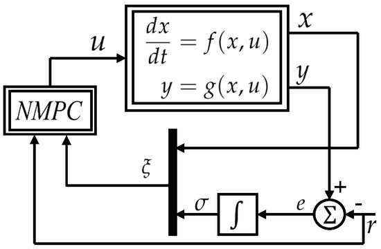
Figure 1.
Integral model predictive controller with system plant.
2.2. Stability
The stability of a system controlled by a model predictive feedback controller can be proven thanks to a Lyapunov function. Ref. [16] shows that nominal stability and feasibility are achieved by choosing a terminal equality constraint appropriately. The terminal equality constraint (9d) is introduced to transform the finite horizon problem into an infinite equivalent horizon problem for which establishing closed-loop stability is easy. This approach, which was developed for linear systems, can readily be extended to the non-linear integral MPC of this paper.
The proof for nominal stability requires that a control input such that at each time instant. If this assumption holds and if the prediction and the plant models are identical, then the closed-loop is asymptotically stable, with its state converging to the desired equilibrium defined by set-point r. The proof can be found in Appendix A.
It is worth noting that model uncertainties affect the system’s equilibrium points, but the presence of the integrator naturally forces the tracking error, e, to converge. Thus, offset-free tracking in the steady state is guaranteed despite the presence of constant disturbances and uncertainties affecting the system providing that closed-loop stability is preserved.
2.3. Non-Linear Model Predictive Control Algorithm
Optimisation problem (9a)–(9d) can be solved efficiently with dedicated non-linear quadratic programming solvers. We chose GRAMPC [12] for its C programming language implementation, which provides computational efficiency, and for its simple interface with Matlab and Simulink. GRAMPC uses an augmented Lagrangian method in which the inequality constraints are converted into equality constraints. The optimisation problem is then transformed into an unconstrained optimisation problem consisting of the original cost function plus a quadratic penalty function term. This approach presents the advantage of being able to deal with numerically ill-conditioned problems [12].
GRAMPC requires analytical expressions of the Jacobian matrices and . The gradients of the cost, , with respect to and u also need to be passed to the solver. These are given by
3. The Coupled Water Tank System
This section introduces the design of an integral non-linear model predictive feedback controller for a coupled, non-linear water tank system. The integral model predictive controller will be tested both in simulations and as part of a physical laboratory experiment.
3.1. The Water Tank Model
The water tank system in this paper consists of two interconnected tanks, shown in Figure 2.
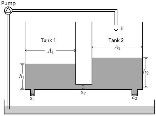
Figure 2.
The coupled tank system.
The dynamics of the coupled tank system are
where and are the water levels in Tank 1 and Tank 2, respectively. u is the input flow to Tank 2 supplied by the pump, and w is the disturbance input. denotes the sign function. and are the cross-sectional areas of the two tanks and of the two outlets, . Water flows into the tank of the lowest level through the connecting pipe of cross-sectional area . The aim of the control system is to control the water level of Tank 1.
3.2. Parameters and Uncertainties
The plant parameters are those of a laboratory experiment developed at the University of Leicester, shown in Figure 3.
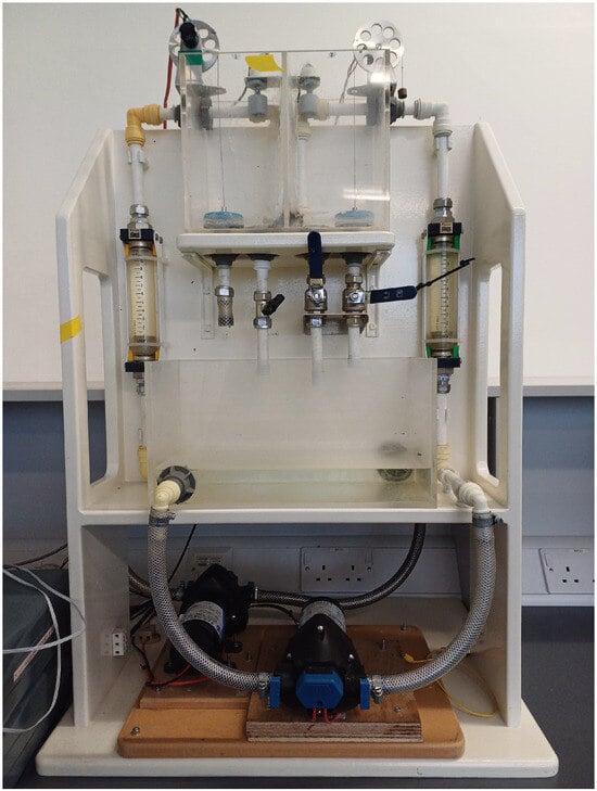
Figure 3.
The coupled tank experiment.
The system’s parameters are determined experimentally and expressed as
where , , , , and are the measured parameter values, and , , , and are the parameter uncertainty weights, , . This model takes into account the irregularities in the tanks’ cross-sectional areas (as these vary with height) and pipe leakages. We assume that the cross-sectional area uncertainties are and the uncertainty of the connecting pipe is . The values of these parameters are given in Table 1.

Table 1.
Coupled tank parameters.
3.3. Constraints
The maximum capacity of the pump is or . Thus, the control input constraints are and , or . The water tank water levels are limited to , i.e., , where , . The terminal equality constraint (9d) is forcing the final state to be equal to the desired equilibrium state. This mechanism is used to ensure nominal stability (see, e.g., [3]).
3.4. The Jacobian Matrix
The Jacobians of the state equation, for , are given by
and
Note that the Jacobian is not defined when or or . In practice, the terms (resp., and/or ) will be replaced by if (resp., and/or ) where is a small positive number.
3.5. Tuning and Simulation Results
The weighting matrices and R are the tuning parameters that determine the closed-loop performance. Increasing the input weighting R and the values of and reduces overshoot and results in smoother but slower responses. A higher value of leads to faster tracking responses but may cause the responses to overshoot.
The prediction horizon, denoted as T, is a critical tuning parameter for model predictive control (MPC), as it directly impacts the stability of the closed-loop system. A short prediction horizon can lead to infeasibility or instability, while a too large prediction horizon is undesirable due to the increased computational burden and potential numerical instability. The selection of the prediction horizon T involves a process of trial and error until satisfactory stability, robustness and performance are achieved.
A prediction horizon T of 50 s is used in (9a)–(9d). The system is discretised with the sampling period . The weighting matrices are chosen as , .
3.5.1. Simulation Results for the Nominal Plant
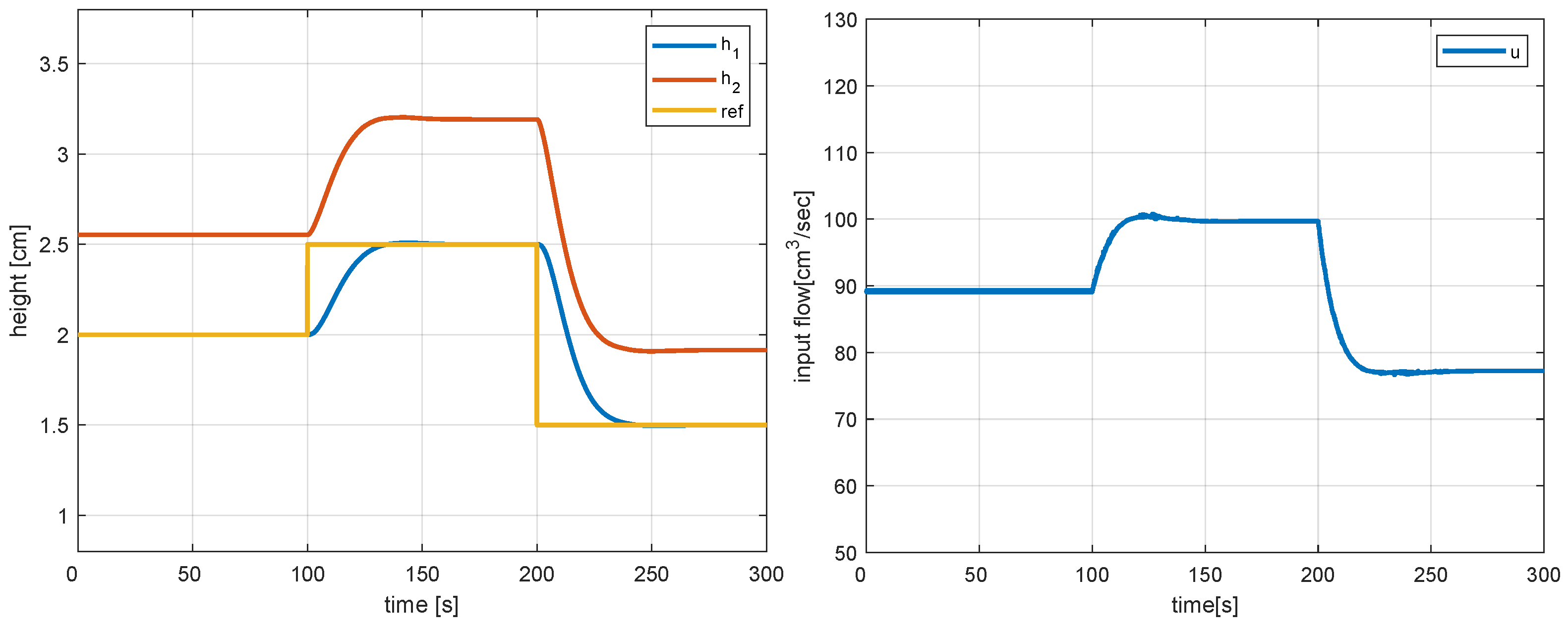
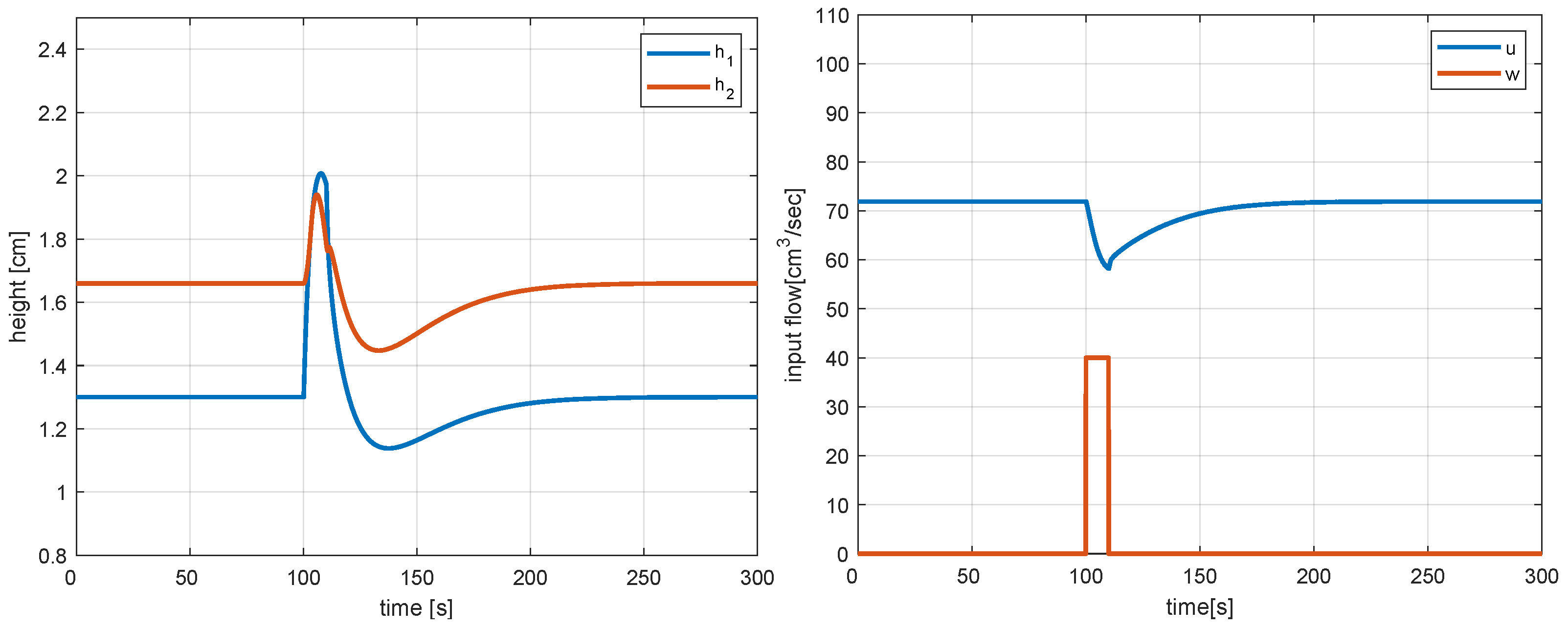
Figure 4 shows the responses corresponding to the nominal plant when a piece-wise constant set-point is applied. One can see that the responses are well damped and that offset-free tracking is achieved in the steady state. The responses corresponding to an impulse, w, as it applies to Tank 1 are shown in Figure 5. One can see that the disturbed state returns rapidly to its initial value with no steady-state error.
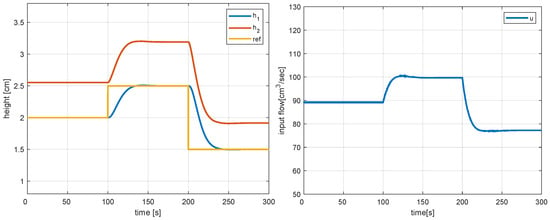
Figure 4.
Tracking responses (left) and corresponding control action (right) with the non-linear model predictive controller for the nominal model.
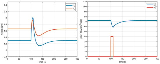
Figure 5.
Disturbance rejection responses and corresponding control action with the non-linear model predictive controller for the nominal model in simulation.
3.5.2. Simulation Results for the Uncertain Plant
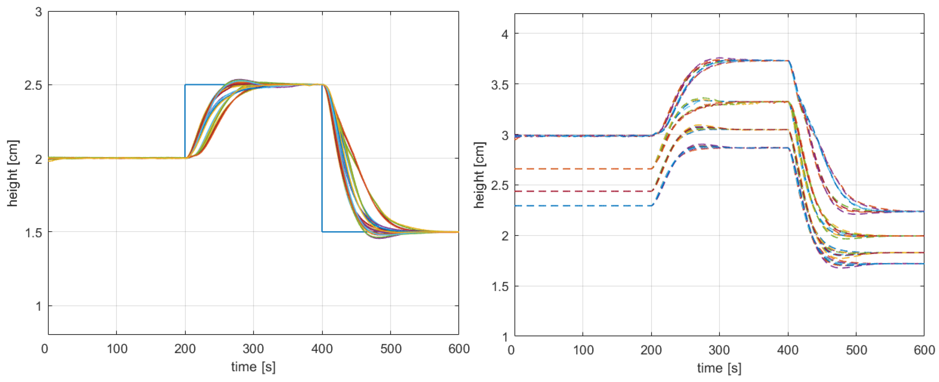
This section presents the responses for a family of 32 coupled tank systems corresponding to uncertainties , . Figure 6 shows the tracking responses for the plant family obtained from the uncertain model. The responses are dispersed due to the uncertainties. Despite this, the responses are well damped, and offset-free tracking is achieved. This shows that integral action enables us to achieve steady-state tracking in the presence of model uncertainties.
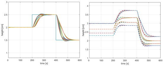
Figure 6.
Responses of Tank 1 (left) and Tank 2 (right) for the non-linear plant family.
3.6. Real-Time Application
This section details the real-time implementation of the non-linear model predictive feedback controller from this paper. The main limitation of implementing the proposed control scheme on hardware is that the non-linear programming solver based on GRAMPC can be challenging to implement on low-cost microcontrollers due to memory limitations. We chose to use an Arduino Mega 2560 as a communication interface between the PC running Matlab and Simulink and the physical system, as illustrated in Figure 7. The Arduino’s digital I/O ports are connected to the sensors and receive the system states from the analog pins. The sensor readings are transmitted to the PC via a USB connection and captured in Simulink using a dedicated block from the Instrument Control Toolbox. The control action computed by GRAMPC is transmitted to the Arduino via the USB connection. The control action is then converted by the Arduino into a PWM signal, which is then applied to the pump DC motor amplifier. This setup allows for the full use of the computational power of the PC despite the implementation being low-cost. The sampling time, , is fixed and set at s.

Figure 7.
Hardware implementation.
3.6.1. Real-Time Results for Tracking and Disturbance Rejection
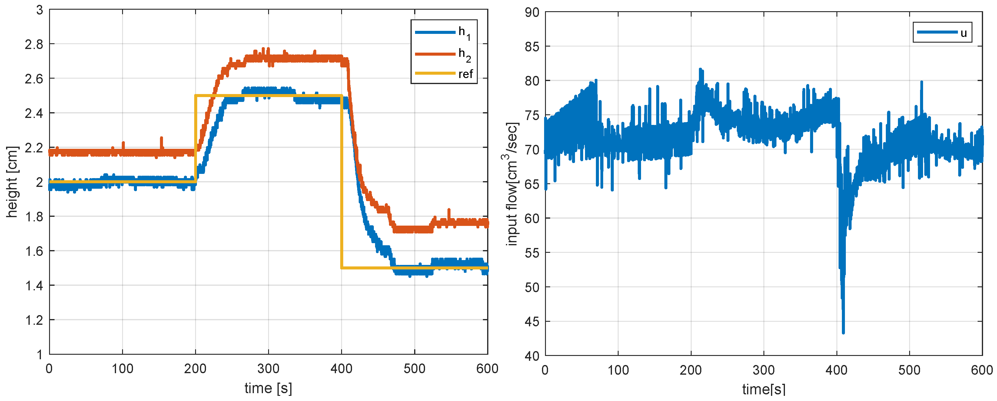
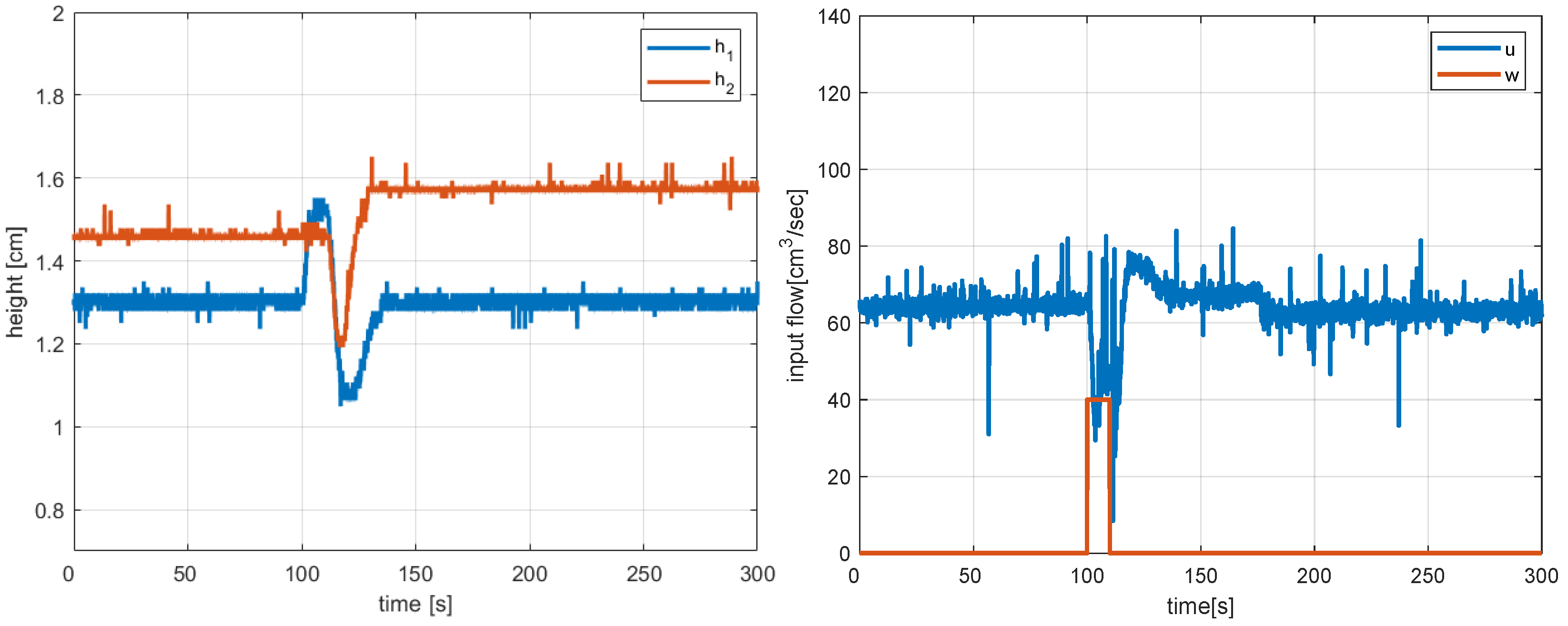
Figure 8 and Figure 9 show the real-time responses and control corresponding to the tracking of a piece-wise constant set-point and a constant disturbance realised by applying a water flow into Tank 1 for . In both cases, the responses are fast, and offset-free tracking of Tank 1 is achieved.
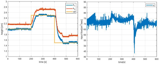
Figure 8.
Real-time tracking responses and corresponding control action with non-linear model predictive controller.
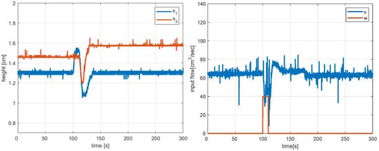
Figure 9.
Real-time disturbance rejection and control action with non-linear MPC controller.
3.6.2. Comparison between NMPC and PID
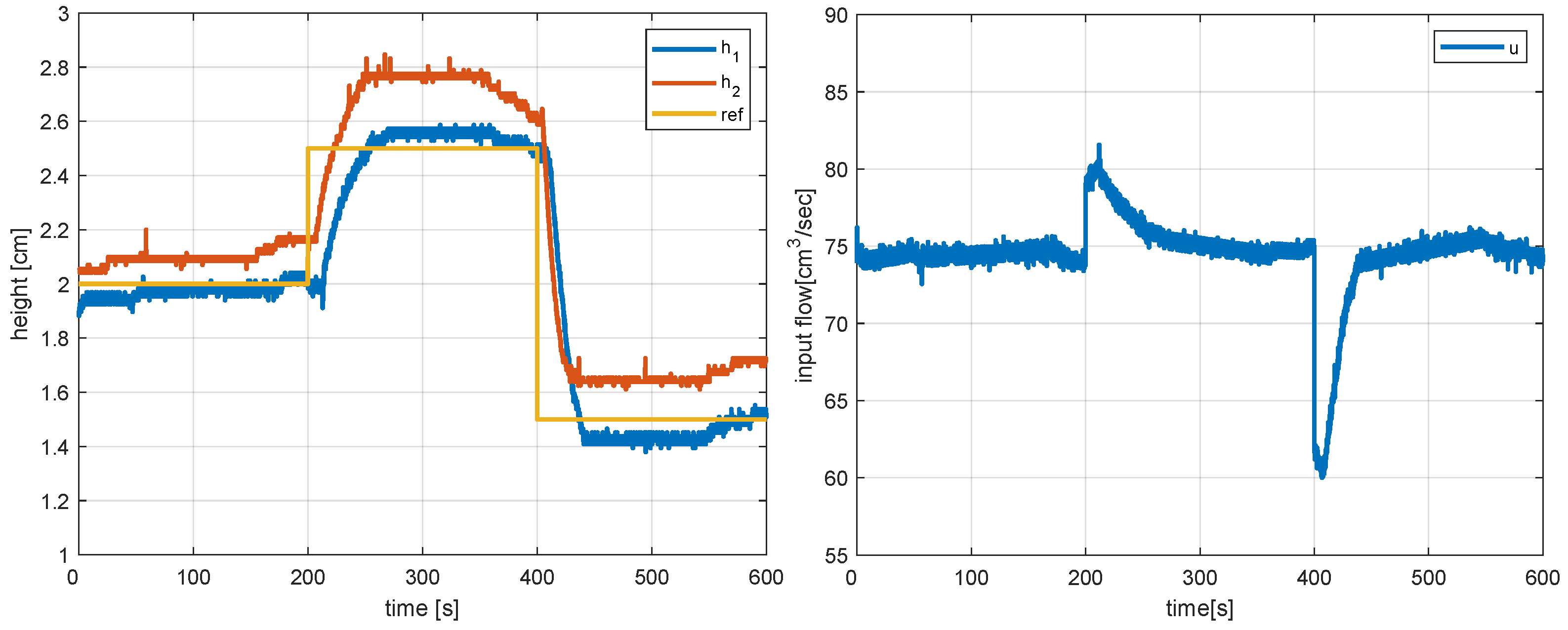
This section compares the effectiveness of the proposed non-linear integral MPC with that of a PID controller. PID controllers are the most commonly used controllers and are usually designed and tuned by linearising around an equilibrium point. Figure 10 displays the responses obtained by a PID controller with proportional, integral and derivative gains , and . One can see that the responses with the PID controller are generally slower than those of the MPC controller. The non-linear integral MPC feedback controller works better than the PID controller because it takes advantage of the non-linear model, while the PID controller can only perform well around the equilibrium based on which it has been tuned.

Figure 10.
Real-time tracking responses and control action with a PID controller.
The root mean square (RMS) of the tracking error for Tank 1, , between instants and is defined as
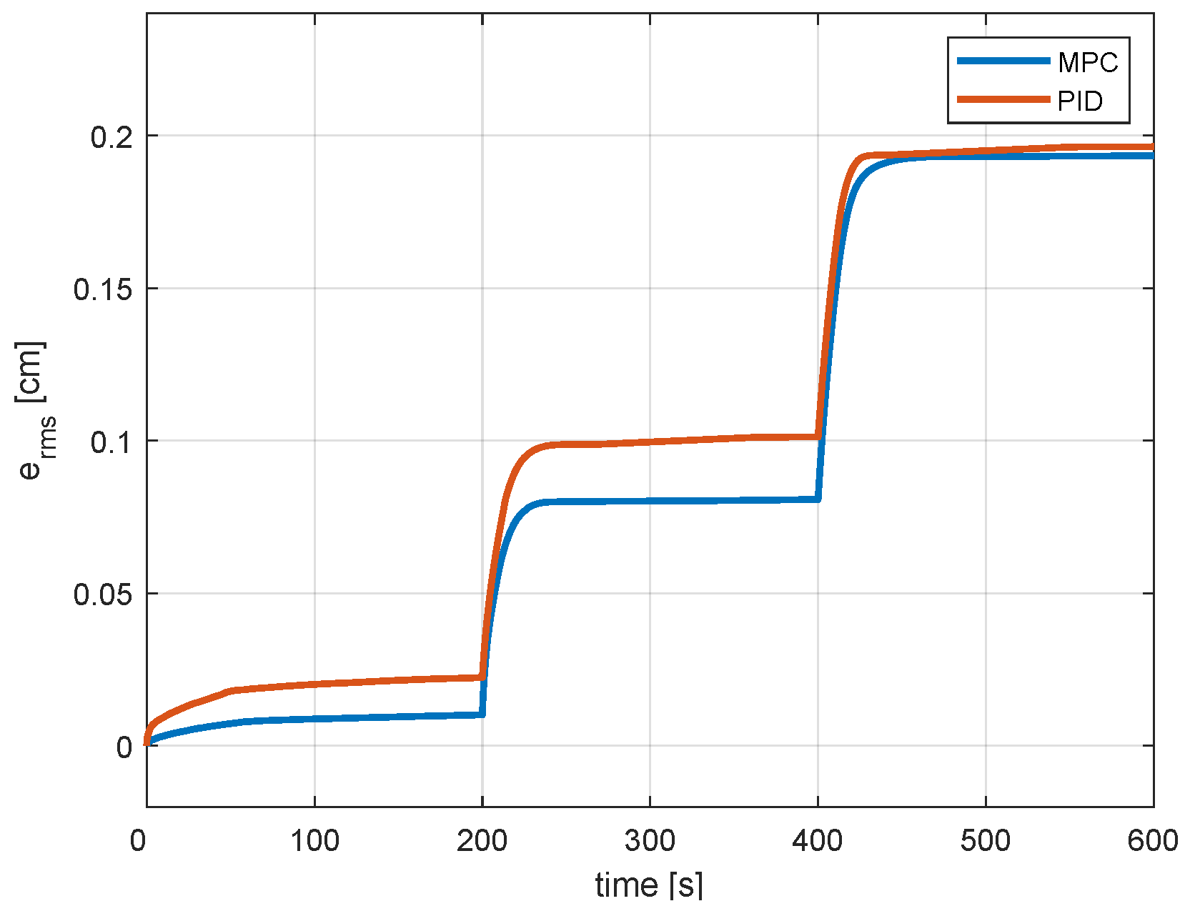
The RMS signals obtained with the PID and NMPC controllers for the set-points shown in Figure 8 are shown in Table 2 and Figure 11. We can see that the MPC controller generally performs better than the PID controller. As shown in Figure 10, the responses obtained with the PID controller are less consistent than those of the NMPC controller, and it takes longer for the PID controller to eliminate the steady-state error.

Table 2.
Real-time tracking performance comparison.
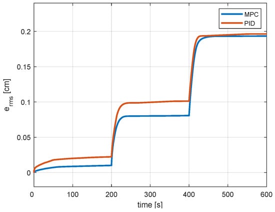
Figure 11.
The RMS signals for the MPC and PID controllers.
4. Conclusions
This paper presents a non-linear integral model predictive controller design for offset-free tracking. The proposed controller design methodology is designed to work with uncertain, non-linear, constrained systems, assuming that the nominal model and the system’s Jacobian matrices are available to the designer. This approach is based on classical control ideas which offer the advantages of not requiring observers when the system states are available and simplicity over the approaches in the literature. The problem in this paper is formulated as a continuous-time optimisation problem and solved using an augmented Lagrangian gradient optimisation approach. It is shown that the resulting controller ensures offset-free tracking in the presence of constant parametric uncertainties and piece-wise constant disturbances that do not destroy the stability thanks to integral action. Analysis of the closed-loop stability is based on a Lyapunov function. The proposed controller is experimentally tested on a non-linear, multivariable, two-tank system.
One issue with the current approach is that the integrator state may be affected by windup. Future work will focus on combining the non-linear integral MPC from this paper with an anti-windup technique.
Author Contributions
Conceptualisation, H.Z. and E.P.; methodology, H.Z. and E.P.; software, H.Z.; validation, H.Z. and E.P.; formal analysis, H.Z. and E.P.; investigation, H.Z. and E.P.; resources, H.Z. and E.P.; data curation, H.Z. and E.P.; writing—original draft preparation, H.Z.; writing—review and editing, E.P.; visualisation, H.Z. and E.P.; supervision, E.P. All authors have read and agreed to the published version of the manuscript.
Funding
This research received no external funding.
Data Availability Statement
The data are contained within the article.
Conflicts of Interest
The authors declare no conflicts of interest.
Appendix A
A discretised version of system (8) is
Consider the optimisation problem at instants i and , and let be the optimal control input sequence minimising at instant i:
At , the control input sequence is constructed. The cost of is then
where
Since is not the optimal control input sequence,
Therefore, is monotonically decreasing, i.e., . is then a Lyapunov function for the closed-loop, and the equilibrium set-point is asymptotically stable.
References
- Pannocchia, G.; Gabiccini, M.; Artoni, A. Offset-free MPC explained: Novelties, subtleties, and applications. In Proceedings of the 5th IFAC Conference on Nonlinear Model Predictive Control NMPC 2015, Seville, Spain, 17–20 September 2015; IFAC-PapersOnLine. Volume 48, pp. 342–351. [Google Scholar] [CrossRef]
- Muske, K.R.; Badgwell, T.A. Disturbance modeling for offset-free linear model predictive control. J. Process. Control 2002, 12, 617–632. [Google Scholar] [CrossRef]
- Rawlings, J. Tutorial overview of model predictive control. IEEE Control. Syst. Mag. 2000, 20, 38–52. [Google Scholar] [CrossRef]
- Morari, M.; Maeder, U. Nonlinear offset-free model predictive control. Automatica 2012, 48, 2059–2067. [Google Scholar] [CrossRef]
- Son, S.H.; Narasingam, A.; Kwon, J.S.I. Development of offset-free Koopman Lyapunov-based model predictive control and mathematical analysis for zero steady-state offset condition considering influence of Lyapunov constraints on equilibrium point. J. Process. Control 2022, 118, 26–36. [Google Scholar] [CrossRef]
- Chen, J.; Dang, Y.; Han, J. Offset-free model predictive control of a soft manipulator using the Koopman operator. Mechatronics 2022, 86, 102871. [Google Scholar] [CrossRef]
- Son, S.H.; Choi, H.K.; Kwon, J.S.I. Application of offset-free Koopman-based model predictive control to a batch pulp digester. AIChE J. 2021, 67, e17301. [Google Scholar] [CrossRef]
- Kumar, P.; Rawlings, J.B.; Carrette, P. Modeling proportional–integral controllers in tracking and economic model predictive control. J. Process. Control 2023, 122, 1–12. [Google Scholar] [CrossRef]
- Limon, D.; Ferramosca, A.; Alvarado, I.; Alamo, T. Nonlinear MPC for Tracking Piece-Wise Constant Reference Signals. IEEE Trans. Autom. Control. 2018, 63, 3735–3750. [Google Scholar] [CrossRef]
- Ruscio, D. Model Predictive Control with Integral Action: A simple MPC algorithm. Model. Identif. Control Nor. Res. Bull. 2013, 34, 119–129. [Google Scholar] [CrossRef]
- Ebirim, K.U.; Lecchini-Visintini, A.; Rubagotti, M.; Prempain, E. Constrained Model Predictive Control With Integral Action for Twin Rotor MIMO Systems. J. Dyn. Syst. Meas. Control 2023, 145, 081006. [Google Scholar] [CrossRef]
- Englert, T.; Völz, A.; Mesmer, F.; Rhein, S.; Graichen, K. A software framework for embedded nonlinear model predictive control using a gradient-based augmented Lagrangian approach (GRAMPC). Optim. Eng. 2019, 20, 769–809. [Google Scholar] [CrossRef]
- Khalil, H. Nonlinear Systems; Pearson Education, Prentice Hall: Hoboken, NJ, USA, 2002. [Google Scholar]
- Slotine, J.; Li, W. Applied Nonlinear Control; Prentice-Hall International Editions, Prentice-Hall: Hoboken, NJ, USA, 1991. [Google Scholar]
- Bryson, A.E.; Ho, Y.C. Applied Optimal Control; Blaisdell: New York, NY, USA, 1969. [Google Scholar]
- Borrelli, F.; Bemporad, A.; Morari, M. Predictive Control for Linear and Hybrid Systems, 1st ed.; Cambridge University Press: New York, NY, USA, 2017. [Google Scholar]
Disclaimer/Publisher’s Note: The statements, opinions and data contained in all publications are solely those of the individual author(s) and contributor(s) and not of MDPI and/or the editor(s). MDPI and/or the editor(s) disclaim responsibility for any injury to people or property resulting from any ideas, methods, instructions or products referred to in the content. |
© 2024 by the authors. Licensee MDPI, Basel, Switzerland. This article is an open access article distributed under the terms and conditions of the Creative Commons Attribution (CC BY) license (https://creativecommons.org/licenses/by/4.0/).


