Abstract
To improve the effectiveness of model predictive control (MPC) in dynamic traffic signal control strategies, it has been combined with graph convolutional networks (GCNs) and deep reinforcement learning (DRL) technologies. In this study, a neural-network-based traffic signal control optimization method under the MPC framework is proposed. A dynamic correlation matrix is introduced in the predictive model to adapt to the dynamic changes in correlations between nodes over time. The signal control optimization strategy is solved using DRL, where the agent explores the optimal control strategy based on pre-set constraints in the future road environment. The geometric structure and traffic flow data of a real intersection were selected as the simulation validation environment, and a joint simulation was conducted using Python and SUMO. The experimental results indicate that in low-traffic scenarios, the queue length is reduced by more than 2 vehicles compared to the selected comparison methods; in high-traffic scenarios, the queue length is reduced by an average of 17 vehicles. Under the actual traffic data of the intersection, the average speed is increased by 6.4% compared to the fixed timing method; compared to the inductive signal control method, it increases from 9.76 m/s to 11.69 m/s, an improvement of 19.7%, effectively enhancing the intersection signal control performance.
1. Introduction
As urban traffic volumes continue to increase, traditional traffic signal control methods have shown significant shortcomings in meeting demand [1,2]. Traditional periodic signal control methods, typically based on fixed time intervals and pre-set signal cycles, are unable to adapt to real-time changes in traffic flow, leading to worsened congestion during peak hours. Although some improved control strategies, such as Self-Organizing Traffic Light (SOTL) and rule-based control methods, have enhanced traffic flow efficiency to some extent, these methods still suffer from low computational accuracy, slow response times, and difficulties in handling complex traffic environments.
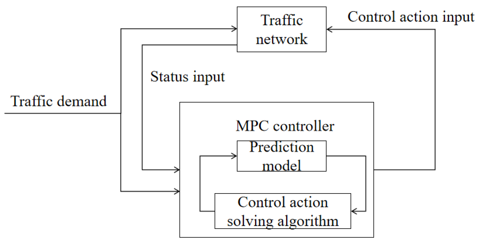
Model predictive control (MPC), as a dynamic optimization control strategy, has garnered widespread attention. The application process of MPC in traffic signal control is illustrated in Figure 1. The system collects real-time traffic data based on the actual demand under the current traffic conditions, including flow, speed, vehicle positions, and other information. This data are then fed into a prediction model, which analyzes historical data and current situations to forecast traffic conditions for a future period. Subsequently, the MPC controller generates the optimal signal control strategy based on these predictions and predefined control objectives. This strategy may involve adjusting signal cycles and green light durations for different directions. The controller then implements these adjustments and updates the signal states. Throughout this process, the MPC algorithm continuously monitors actual traffic conditions and prediction deviations, adjusting control strategies in real time to ensure the effectiveness and adaptability of traffic signals. From the workflow of MPC, it is evident that an accurate traffic flow prediction model and an efficient method for solving control actions are crucial for achieving effective intersection signal control. Therefore, improving traffic flow prediction models and integrating intelligent algorithms into the MPC framework to quickly solve optimal control actions are our work objectives.
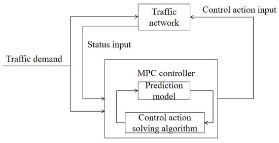
Figure 1.
MPC applied to traffic signal control schematic.
Traffic flow models are used to describe and predict the dynamic behavior of traffic on road networks, including parameters such as vehicle density, speed, and flow. These models can be either macroscopic or microscopic. Hegyi et al. optimized traffic control for highway networks using the METANET macroscopic traffic flow prediction model. Macroscopic models are suitable for describing and predicting the overall behavior of large-scale traffic networks, resulting in satisfactory outcomes for highway traffic control [3]. Stoilova et al. extended the existing “store-and-forward” model by incorporating optimization problems that consider the probability of vehicles, thereby better capturing the stochastic nature of actual traffic flow [4]. Ferrara et al. used an MPC method based on the Cell Transmission Model (CTM) to manage traffic flow by controlling the inflow at ramp entrances. CTM provides a macroscopic description of traffic flow by dividing the highway into multiple cells, which helps simplify the dynamics of complex traffic flows [5]. Sirmatel et al. proposed an MPC method based on the Macroscopic Fundamental Diagram (MFD) for network-level traffic control. The MFD typically features low dispersion and a unimodal characteristic, meaning that flow variations are relatively smooth across different accumulation levels, aiding the controller in achieving smoother and more predictable control outcomes [6]. Wang et al.’s research on the motion state estimation of intelligent vehicles contributes not only to traffic data collection but also to the study of micro-level vehicle behaviors [7]. Moreover, with the development of artificial intelligence technologies such as neural networks, data-driven traffic flow prediction methods have been widely applied. Yang et al. used graph-theory-based methods to capture the spatiotemporal dependencies between adjacent road segments to predict the evolution of traffic states on highway networks. This method remains effective even when extending the prediction time horizon [8]. Ling et al. used an encoder–decoder structure with graph convolutional networks (GCNs) to learn the changing spatial features between traffic sites, extracting these features by integrating spatial and temporal dependencies, which demonstrated superior predictive performance [9]. Hu et al. noted that the spatial dependencies of traffic data arise from different environments and change over time; fully capturing these spatial and temporal dependencies is key to accurate predictions [10]. In traffic networks, different road segments influence each other, and GCNs can effectively utilize these spatial relationships to improve prediction accuracy. The application of GCNs in traffic flow prediction has gained increasing attention from researchers. Compared to other traffic flow models, their superior predictive performance is mainly due to their ability to effectively represent traffic flow characteristics on urban roads in both temporal and spatial dimensions [11,12]. Enhancing the representation accuracy of correlations between traffic flows using graphs is crucial for improving the predictive performance of GCNs, and this is our focus. Typically, the relationships between nodes in a road network can be represented by adjacency matrices or weight matrices. Adjacency matrices use 0 s and 1 s to indicate whether there is a connection between nodes, while weight matrices pre-set the closeness of connections between different road positions using metrics such as distance between nodes. These methods can simply describe the connections between nodes but cannot dynamically change over time, leaving room for optimization in terms of final prediction performance [13,14,15].
Since De Schutter et al. first proposed the MPC method for traffic signal control [16], research on control strategies has primarily focused on three aspects: simplifying nonlinear traffic flow models and network-based MPC methods, linear MPC control methods, and MPC methods considering uncertainties. In their research on simplified nonlinear models, Lin et al. proposed a streamlined nonlinear traffic flow model alongside a network-based MPC method, which demonstrated robust control performance under both balanced and unbalanced traffic conditions [17]. In exploring MPC methods that account for uncertainties, Ye et al. developed a stochastic MPC model to simulate variable traffic demands and random disturbances. They integrated stochastic simulation and neural networks with genetic algorithms to formulate a hybrid intelligent approach for addressing uncertainty optimization challenges [18]. As the complexity of urban road networks increases, modeling traffic signal control problems requires consideration of adjacent intersections and road topology [19]. Additionally, MPC’s reliance on real-time data necessitates high-quality data and sensor accuracy, making the integration of MPC strategies with computational intelligence methods a growing trend. Traditional optimization algorithms, such as Particle Swarm Optimization and Genetic Algorithms, have been widely used to find global optimal strategies. However, these algorithms often suffer from issues of low computational precision and convergence difficulties [20]. With the rise of artificial intelligence, deep reinforcement learning algorithms have shown better adaptability to complex traffic environments, enabling adaptive adjustments according to different traffic conditions and road scenarios. Deep reinforcement learning can learn optimal control strategies from raw data, maintaining efficient signal control under various traffic situations. A Deep Q-Network (DQN) is a reinforcement learning algorithm that combines deep neural networks with Q-learning to address reinforcement learning problems in discrete action spaces [21]. Traffic signal control typically involves discrete action choices, such as changing the states of traffic lights. A DQN effectively handles such discrete action spaces by using Q-values in the network’s output layer to select the best action. Moreover, a DQN employs experience replay to train the neural network stably, meaning it can learn from previous experiences and avoid training instability caused by data correlations. This is particularly important in real-time decision-making environments like traffic signal control.
MPC methods can be categorized based on the type of control architecture into centralized MPC, hierarchical MPC, and distributed MPC [22]. Centralized MPC optimizes signal control strategies across the entire traffic network to achieve global optimal control [23]. Hierarchical control divides traffic signal controllers into multiple levels, where each level controls a specific range of intersections. The higher-level controllers coordinate different levels to achieve global optimization, while the lower-level controllers focus on local optimization for their respective intersections. Distributed MPC, on the other hand, optimizes signal control strategies for each intersection to achieve local optimal control [24]. Pham et al. designed a distributed stochastic MPC method suitable for urban traffic networks, which not only considers the uncertainties in traffic model parameters but also leverages the characteristics of the distributed architecture to enhance the model’s performance in solving optimization problems [25]. Alfonso et al. proposed a novel control architecture that combines distributed reinforcement learning and MPC to address fleet path planning and dynamic driving decisions. This method uses traffic data from each intersection along with a distributed reinforcement learning algorithm to obtain fleet control decisions, providing a robust solution for signal control problems [26]. Current research primarily focuses on the global optimization of urban traffic networks, with relatively insufficient studies on optimizing signal control at individual intersections. The traffic control problems at single intersections are unique and significant because they are fundamental components of the traffic network and have a direct impact on overall traffic flow and congestion. To fully utilize real-time traffic data and improve traffic flow efficiency at intersections, this paper constructs a traffic signal optimization model within the MPC framework based on an improved graph convolution prediction model and a deep reinforcement learning algorithm. This approach leverages the advantages of neural networks in modeling spatiotemporal characteristics of urban traffic, adaptively adjusting control strategies based on real-time traffic data to enhance the overall efficiency of the traffic system. The contributions of this paper are as follows:
- Propose an improved graph convolution prediction model: This model is used to describe traffic flow states, introducing a node dynamic feature extraction module for real-time traffic data. By integrating a GCN and gated recurrent units (GRUs), it enhances the prediction accuracy of spatiotemporal traffic characteristics.
- Optimize traffic signal control strategies using deep reinforcement learning within the MPC framework: A DQN is employed to adaptively adjust control strategies in complex traffic environments, significantly improving the response speed and optimization effectiveness of the signal control system.
- Design an MPC-based traffic signal control algorithm: This algorithm aims to increase the average speed of vehicles passing through intersections and reduce the likelihood of queueing and waiting.
2. Model Predictive Control Framework
MPC is an online control strategy, which means it continually recalculates and updates control inputs. At each time step within the prediction horizon, the control system solves an optimization problem to find the optimal control input that minimizes the cost function while satisfying the constraints. This process iterates iteratively, computing a control sequence at each time step and applying the first control input from that sequence then advancing to the next time step. This process continues, effectively pushing the prediction horizon forward in time.
Implementing a continuous feedback loop between predictive models and MPC controllers involves utilizing the output of the predictive model to update state estimation and inform the decision-making process of the controller. The state vector is represented as , the control input as , and the output of the predictive model as . The estimation of the system state by the predictive model is represented as follows:
where is the estimated state at time step and is the model function of the predictive model, which utilizes the current state and control input to estimate the state.
The MPC controller utilizes the estimated state from the predictive model to make control decisions. The objective of the MPC controller is to minimize the cost function , which depends on the control input , system state , and future state predictions . The cost function is represented as follows:
where is the immediate cost function and is a cost function that depends on the predicted future state .
The MPC controller utilizes a predictive model based on the control input and initial state estimate to estimate future state trajectories, as shown in Equation (3).
where represents the predicted future state trajectory and is the predictive model that uses the current state estimate and control input to forecast future states.
The MPC controller calculates the optimal control input by solving an optimization problem that minimizes the cost function subject to constraints. The optimal control input and associated constraints are shown in Equations (4)–(7):
where represents the optimal control input, and denote control input constraints, and and represent state constraints.
After computing the optimal control input, the MPC controller executes the first control action and propagates the system to the next time step, as shown in Equation (8):
Then, the predictive model provides an updated state estimate for the current time step, as shown in Equation (9):
This updated state estimate is used as the initial state estimate for the next MPC iteration, as shown in Equation (10):
This process is iterated at each subsequent time step, establishing a continuous feedback loop between the MPC controller and the environment. Within this loop, the predictive model perpetually updates the state estimate, thereby informing and refining the MPC controller’s decisions at each ensuing time step.
3. Dynamic Spatiotemporal Correlation Graph Convolution Prediction Model
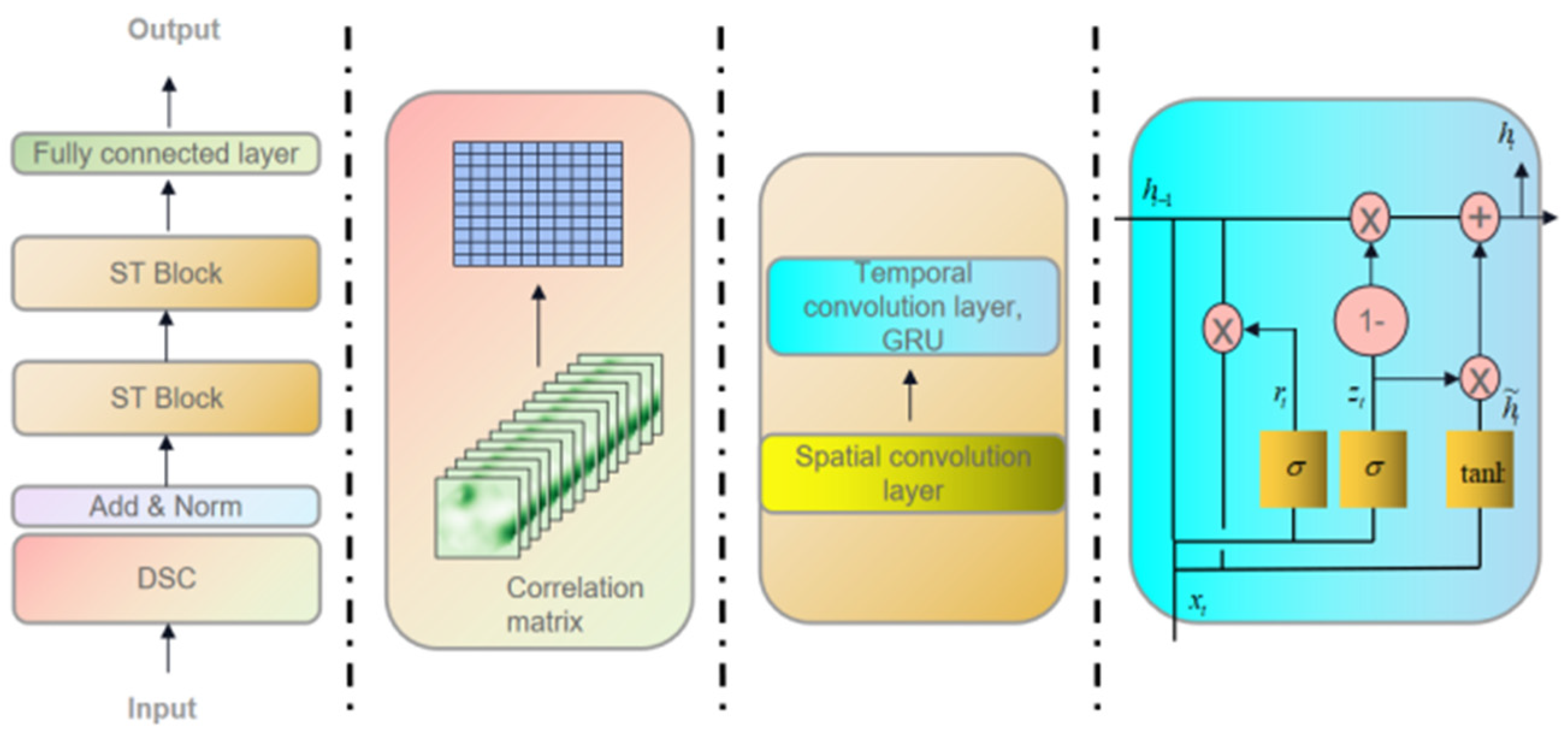
The overall architecture of the prediction model is shown in Figure 2. The flowchart on the far left represents the process of traffic data transmission within the predictive model. The three diagrams on the right are distinguished by different colors, corresponding to the three modules in the predictive model: a dynamic correlation matrix fusion module for representing relationships between nodes, a graph convolutional module for extracting spatial correlations from the data, and a gated recurrent unit (GRU) module for extracting temporal correlations.
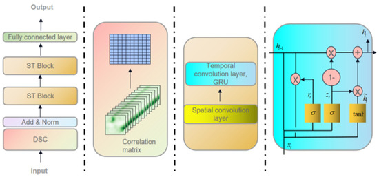
Figure 2.
The model structure of dynamic spatiotemporal correlation graph convolution network (DSCGCN).
The spectral method of the GCN transforms node features into the spectral domain, performs convolution operations using filters, and then transforms the results back into the spatial domain. This process is analogous to the Fourier transform for time series or image data. The GCN applies convolution operations directly to graph-structured data by operating on the graph’s adjacency matrix and node feature matrix. With an increasing number of graph convolutions, the GCN can learn to capture complex spatial patterns and dependencies in the data. The convolution process of the graph is represented as follows in Equation (11):
where is the feature matrix at each layer; is the learnable weight matrix; is the normalized adjacency matrix with added self-connections; is the adjacency matrix; is the identity matrix; is the degree matrix; and is a nonlinear activation function.
The gated recurrent unit is a type of recurrent neural network architecture that can more effectively capture long-term dependencies in time series data compared to traditional RNNs. In traffic prediction tasks, temporal features are crucial for understanding the dynamics of traffic flow, so the GRU is integrated into the predictive model to enhance its capability to handle temporal features. The GRU includes gating mechanisms that retain or update the hidden state at each time step. The GRU architecture consists of three main components: the update gate, the reset gate, and the hidden state [27]. These gates control the flow of information through the network, allowing the GRU to adaptively learn which information to retain or discard at each time step. The update process of the GRU is represented by Equations (13)–(16):
where represents the reset gate, represents the update gate, and represents the hidden state.
The hidden state is updated based on the input data, the previous hidden state, and the outputs of the update and reset gates. It captures the essential information of the input sequence and is used to make predictions at each time step. The update gate determines how much of the previous hidden state should be retained and whether to update the current input and the previous hidden state information into the candidate hidden state. It uses an activation function to output values between 0 and 1, which act as weights for the linear combination of the previous hidden state and the candidate hidden state.
The reset gate regulates the extent to which the previous hidden state is utilized in computing the candidate hidden state. Similar to the update gate, it employs an activation function to generate values ranging between 0 and 1. The reset gate allows the GRU to discard past irrelevant information when calculating the new hidden state.
The adjacency matrix in graph convolutional networks represents the relationships between nodes. Since the relationships between nodes in a road network dynamically change over time, a dynamic correlation matrix fusion module is introduced in the predictive model to represent real-time relationships between road network nodes. This module calculates the correlations between nodes at different times based on the feature matrix and generates a series of correlation matrices. The fused correlation matrix is used as the new adjacency matrix input to the model. The generation of the correlation matrix is represented as follows in Equation (17):
where represents the number of nodes, and represent features of different nodes, and represents the selected length of the time series.
4. Control-Action-Solving Model Based on Deep Reinforcement Learning
The DQN can adapt to constantly changing traffic patterns and continuously update its policy based on interactions with the environment. Implementing adaptive traffic signal control using the DQN first requires constructing an environment that interacts with the agent. This environment should include a state representation (S) that captures the current state of the traffic system, an action space (A) representing the set of actions that the traffic signal controller can take, and a reward function (R) that quantifies the performance of the traffic signal controller. The agent selects a series of actions in the action space based on the system state, and in the context of traffic signal control, it receives rewards by altering phase durations, cycle times, and sequences, repeating this process continuously. The goal of the agent is to maximize cumulative rewards, optimizing intersection throughput efficiency.
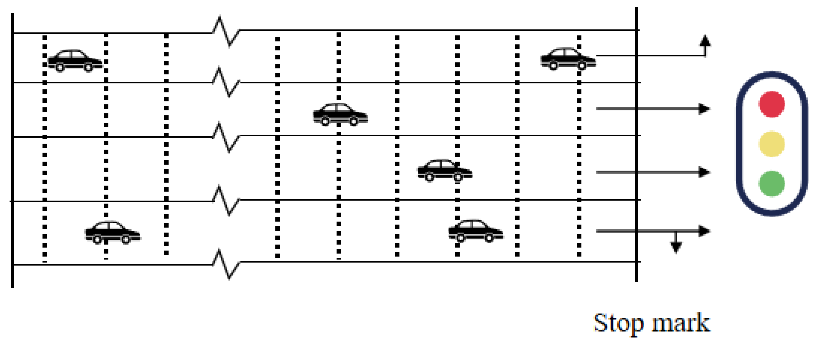
Regarding the state representation, when optimizing traffic signals at a specified intersection using the DQN algorithm, the entry lanes are discretized into 20 small units distributed across all lanes. Ten units are allocated to the leftmost lane, while the remaining ten units are shared among the other lanes, forming the basic elements of the state space. The entire state space of the intersection consists of real-time information about the occupancy status of each unit among the 80 discrete units, effectively identifying the presence or absence of vehicles. The specific distribution is illustrated in Figure 3.

Figure 3.
The process of lane status recognition. The dashed lines in the figure represent cells that detect the presence of vehicles; The broken line indicates the omitted part, because the lane is longer; The arrow indicates the direction in which the vehicle is turning.
Actions: Traffic signal lights select different actions based on different traffic states to guide vehicles to pass in an orderly fashion and reduce intersection queue delays. During operation, the agent selects signal light phases from four predefined phases. The initial duration of each phase is 10 s. A yellow phase, lasting 3 s, is activated when the phase changes. For example, at a given moment, if the traffic signal at the intersection is in phase one, the sequence of signal light actions executed by the agent would be “GGGGrrrrrrGGGGrrrrrr”. This sequence is evenly decomposed into four subsequences, each representing the signal light status of the entrance lane in the same direction. The first subsequence is “GGGGr”, where G represents a green light signal, and r represents a red light signal, indicating that vehicles can proceed straight or turn right at the intersection. Similarly, the signal light action sequences for all remaining lanes are defined to form action space A. The action space of the proposed model is defined as A = {a1, a2, a3, a4}, where the specific meanings of the four predefined phases are as follows:
North–south straight (a1): Green signal lights for north–south entrance lanes direct vehicles to turn right or proceed straight.
North–south left turn (a2): Green signal lights for north–south entrance lanes direct vehicles to turn left.
East–west straight (a3): Green signal lights for east–west entrance lanes direct vehicles to turn right or proceed straight.
East-west left turn (a4): Green signal lights for east–west entrance lanes direct vehicles to turn left.
Reward: The reward function, as a crucial component guiding the training process of the model, plays a central role in deep reinforcement learning models. It is a special mechanism used to shape the behavior of the agent to achieve the desired optimization objectives. During the training process, the model computes the cumulative waiting time of vehicles when executing various actions. The time interval for each vehicle is detected from the initial time generated on the road to the time it passes through the intersection. Cumulative waiting time refers to the duration when the speed of the vehicle is zero within the detected time interval. Minimizing the cumulative waiting time is set as the optimization objective, which is transformed into positive rewards for the agent. The specific expression of the reward function is as follows in Equation (18):
where represents the cumulative waiting time before executing the action and represents the cumulative waiting time after executing the action. Normalizing the reward function can enhance numerical stability during the training process, especially when considering the issues of gradient explosion or vanishing gradients in deep reinforcement learning models. Therefore, in this study, the reward function is normalized.
The update mechanism of the model is crucial for the continuous learning and updating of the agent. Specifically, the agent learns the state-action function through deep neural networks to update action values. The specific update mechanism is represented as follows in Equation (19):
where represents the current reward, represents the discount factor, represents the next state, represents the action chosen at the next state, and is the value of the next state estimated using the target network.
The neural network adopts a fully connected approach with 80 neurons in the input layer, 5 hidden layers each with 400 neurons, and an output layer with 4 neurons representing the four possible actions. The agent’s experiences are stored in an experience pool. At the end of each scene, the agent extracts multiple batches of random samples from the experience pool and then uses the Q-learning equation to update action values. These updated action values are used to train the neural network. Through this process, the neural network incrementally learns more effective action strategies, thereby enhancing the agent’s performance. The advantage of this update mechanism lies in the agent’s ability to continually adjust and optimize its behavior strategy based on its accumulated experiences and acquired knowledge.
5. Simulation and Discussion
The simulation platform used during the experiment is SUMO (Simulation of Urban MObility). SUMO is an open-source, microscopic urban traffic simulation package widely applied in traffic and mobility simulation research. It is designed to simulate large-scale traffic networks and provide detailed analysis of traffic flow, vehicle movement, and traffic management. Various traffic signal control schemes, including fixed time control, adaptive signal control, and rule-based signal control, can be simulated in SUMO, which aligns with our research requirements. Its open architecture and modular design allow users to extend its functionalities as needed. For instance, custom vehicle models and traffic signal algorithms can be written by users. The rich and powerful features of SUMO make it popular in the field of traffic simulation [28,29]. As an open-source project, SUMO has an active community of developers and users. The source code can be freely accessed, modified, and extended according to individual needs. Based on a microscopic simulation model, SUMO can accurately simulate the behavior and interactions of individual vehicles, which ensures a high degree of credibility in its simulation results for both research and practical applications. To quantitatively analyze the robustness of SUMO simulation results, 10 pre-experiments with different random seeds were conducted while keeping other parameters constant before the validation experiment began. These experiments produced multiple sets of data on the average speed and queue length of vehicles at the intersection over time using the MPC-NN control method proposed in this study. The mean and standard deviation of these 10 sets of experimental results were calculated and are presented in Table 1. The consistency between each set of data was quantitatively assessed using the concordance correlation coefficient (CCC), which is calculated as shown in Formula (20), where represents the Pearson correlation coefficient, and represent the standard deviation of the two sets of data, and and represent the mean.

Table 1.
Consistency correlation coefficient experimental results.
In this process, the Pearson correlation coefficient was also utilized, and its results are similarly displayed in Table 1. The range of the consistency correlation coefficient is between −1 and 1, where 1 indicates complete consistency among multiple sets of simulation results and 0 indicates no consistency between the simulation results. From the experimental results, it can be observed that after applying the control method proposed in this paper in SUMO, the consistency correlation coefficients of the two indicators mostly fall between 0.6 and 0.75. Therefore, it is considered that the results of this simulation software are stable and can be used as a simulation tool to verify different traffic control methods.
The simulation verification combines actual road network data with synthetic data to validate the control effectiveness of the model under different traffic densities. The calculations are already being performed on laptops equipped with an Intel Core i57300HQ processor (Santa Clara, CA, USA) and gtx1050 graphics card (Nvidia, CA, USA) under a 64-bit operating system.
Actual road network data are selected from the traffic flow data at the intersection of Moganshan Road and Jiaogong Road. At this intersection, there are five entry lanes each for the east–west and northbound directions and four entry lanes for the southbound direction. Each lane is 700 m long. For the north and west entry lanes, the two leftmost lanes are designated for left turns, the rightmost lane is for right turns, and the two middle lanes are for straight. For the east and south entry lanes, the leftmost lane is for left turns, the rightmost lane is for right turns, and the middle lane is for straight. The road environment established in the SUMO software (1.19.0) is depicted in Figure 4.
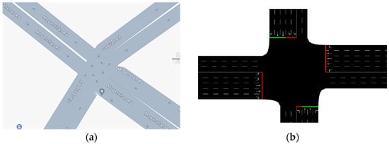
Figure 4.
Simulation of the road environment. (a) The study focuses on the intersection of Moganshan Road and Jiaogong Road in Hangzhou; (b) the simulation scenario in SUMO.
For synthetic data, each simulation round is conducted under two traffic scenarios: high and low traffic flows [30]. A high-traffic-flow scenario refers to situations where congestion begins to appear on the road, while a low-traffic-flow scenario refers to situations where traffic flows freely. It is assumed that the arrival times of vehicles follow a Weibull distribution with a shape parameter k of 2. This distribution is characterized by a rapid increase from the initial time, reaching a peak in the middle, and then gradually decreasing, which is more consistent with the arrival patterns of vehicles in real-world scenarios. The probability density function of the Weibull distribution is expressed as follows in Equation (21):
where represents the random variable, represents the scale parameter, and represents the shape parameter.
During the simulation process, traffic signal control actions are dynamically adjusted by the intelligent agent based on the predicted future road conditions. During the training of the model, settings for hyperparameters need to be configured. The specific parameter settings for the simulation experiments in this paper are shown in Table 2.

Table 2.
Summary of experimental parameter settings.
To validate the effectiveness of the model, the method proposed in this paper (MPC framework based on neural network, MPC-NN) is compared with other common traffic signal control methods. The methods used for comparison are the fixed timing (FT) control method and the Split Offset Traffic Light (SOTL) method from the induction-based traffic signal control. The specific control logic for the comparison methods is explained as follows.
Fixed timing (FT) control method: The fixed timing method is the most common signal control method. Signal phases are pre-set, with each phase automatically transitioning to the next after its designated time expires. The order and duration of phases remain fixed. In the simulation process, the durations for the through phase and the left turn phase are 27 s and 6 s, respectively. There is a 3-s yellow light interval during phase transitions.
Induction-based traffic signal control method: This method relies on sensors pre-set near stop lines on the road to collect vehicle information, combined with locally defined rules for phase transitions. In this paper, a commonly used self-organizing phase rule, the Self-Organizing Traffic Light (SOTL) method [31], is chosen. The SOTL control algorithm is based on a pre-set queue length threshold. Road sensors detect the queue length of vehicles on the inbound lanes. When the queue length is below the pre-set threshold, signal phases switch according to the predetermined normal sequence. However, when the queue length exceeds the threshold, higher priority is given to the corresponding direction’s lane. If multiple lanes have queue lengths exceeding the threshold simultaneously, the queue lengths of each lane are compared, with lanes having more queued vehicles receiving higher priority. Experimental results indicate that setting the queue length threshold to 4 yields better simulation results in terms of average speed and queue length.
Meanwhile, in the simulation validation section, this paper selects average speed and queue length as the evaluation metrics. The “.vehicle.getSpeed” method of the TraCI interface is utilized to obtain the speed of each vehicle passing through the intersection during the simulation process, and then the average speed is calculated and outputted. The “.edge.getLastStepHaltingNumber” method is used to obtain the total queue length within the intersection in the simulation scenario. In the simulation results, a higher average speed indicates better performance, as it signifies vehicles passing through the intersection at a faster rate. Conversely, a smaller queue length is preferable, indicating that the traffic signal control system effectively balances the traffic flow demands from all directions.
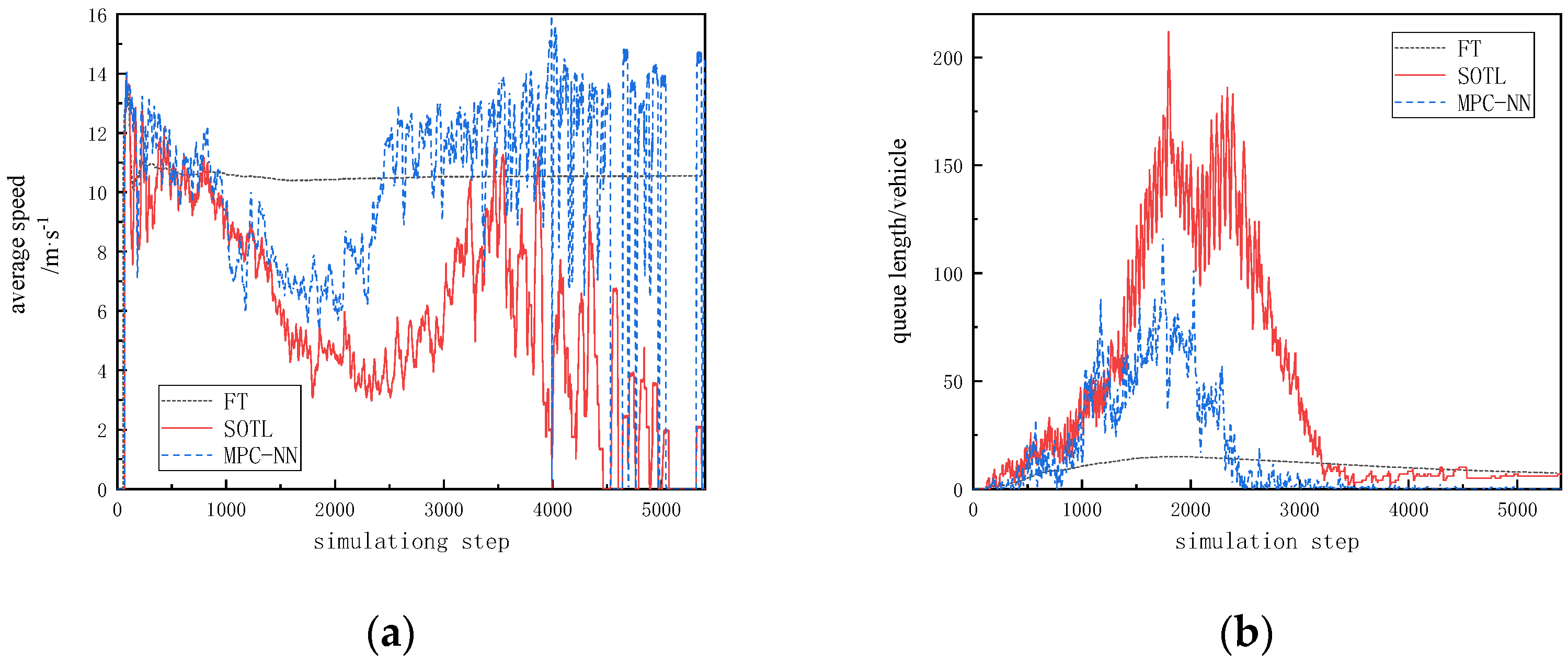
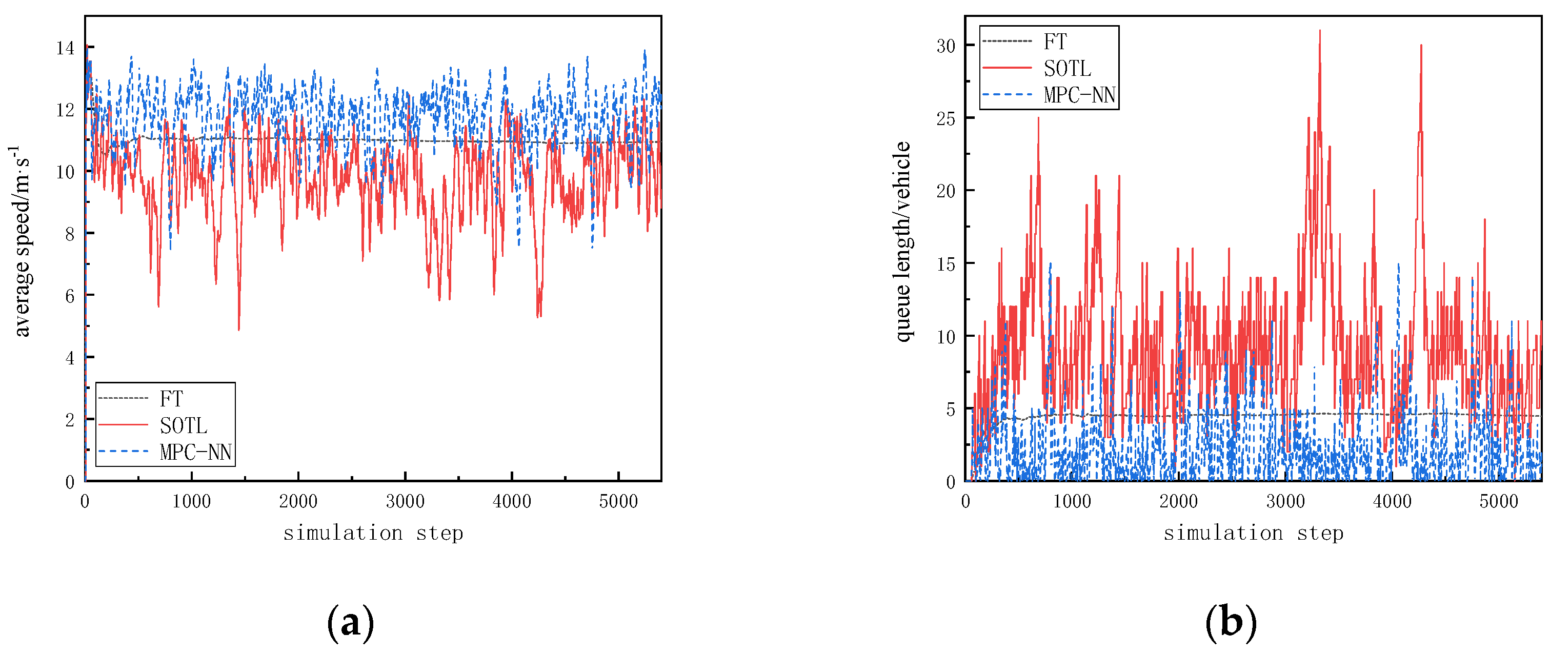
Overall, the evaluation metrics of the three models perform better in low-flow scenarios compared to high-flow scenarios. The simulation results for average speed and queue length in low-flow scenarios are shown in Figure 5, while those in high-flow scenarios are illustrated in Figure 6. Specific metrics are summarized in Table 3. In low-flow scenarios, the average speeds for all control methods are concentrated between 9 and 13 m/s, while in high-flow scenarios, average speeds mostly fall below 14 m/s. The variation in queue length is more pronounced, with significantly longer queues in high-flow scenarios compared to low-flow scenarios.
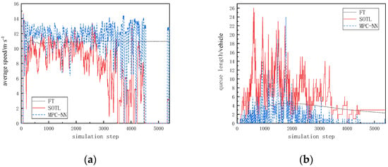
Figure 5.
Simulation results in low-traffic scenarios. (a) The trend of average speed changes under low-traffic-flow scenarios; (b) the trend of queue length changes under low-traffic-flow scenarios.

Figure 6.
Simulation results in high-traffic scenarios. (a) The trend of average speed changes under high-traffic-flow scenarios; (b) the trend of queue length changes under high-traffic-flow scenarios.

Table 3.
The result summary of synthetic data in simulation experiment.
The proposed MPC-NN method shows improvements across various metrics in both scenarios compared to the other two methods. From the figure, it can be observed that in low-flow scenarios, the average speed is generally higher with the MPC-NN method compared to both the fixed timing method and the SOTL method, with an increase of 8% compared to the fixed timing method and 72.7% compared to the SOTL method. Regarding queue length, there is a reduction of 165% compared to the fixed timing method and nearly five vehicles compared to the SOTL method. In high-flow scenarios, the proposed method outperforms the SOTL method in optimizing queue length, with a reduction of nearly 30 vehicles.
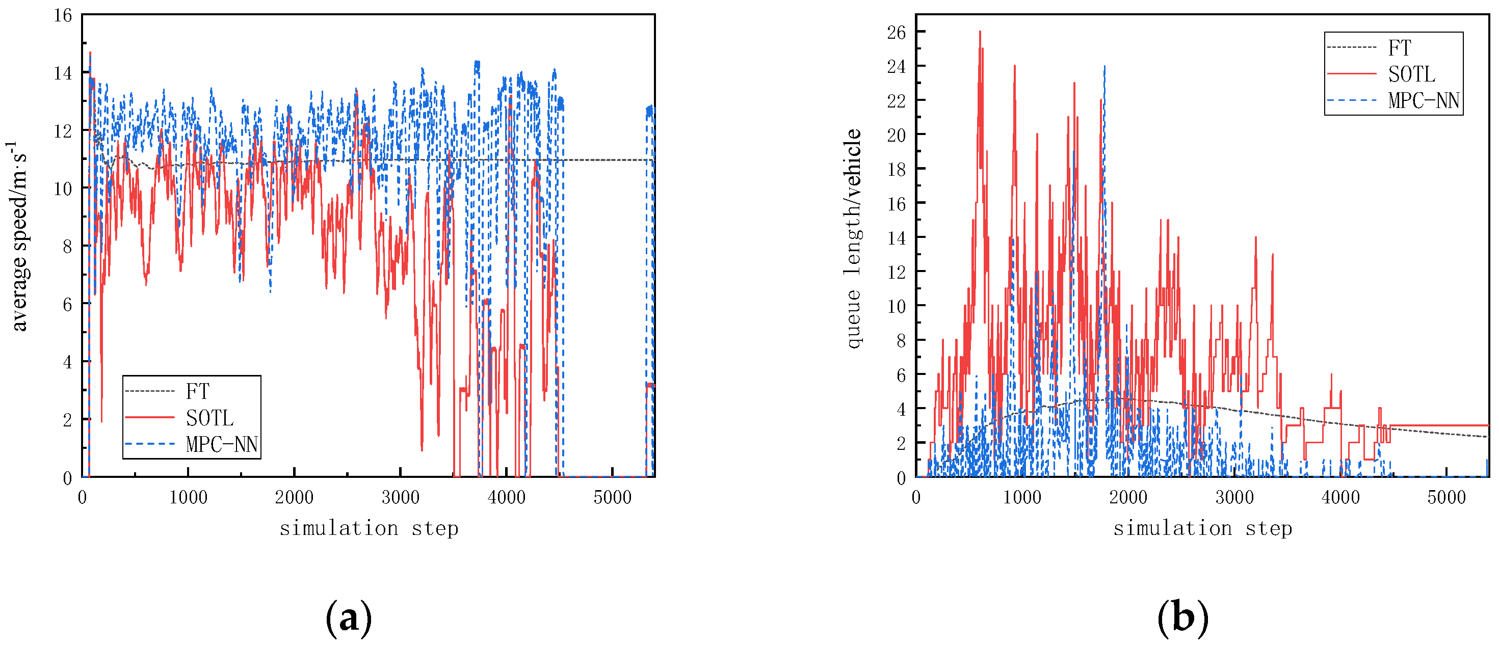
Using real data for the simulation, the results indicate that the proposed MPC-NN method outperforms the other two methods in terms of control effectiveness. The specific simulation results are shown in Figure 7, with metrics summarized in Table 4. In real-world scenarios, under the proposed method, the average speed increases by 6.4% compared to the fixed timing method and by 19.7% compared to the SOTL method. Regarding queue length, there is a significant reduction compared to both the fixed timing method and the SOTL method, with decreases of two vehicles and seven vehicles, respectively.
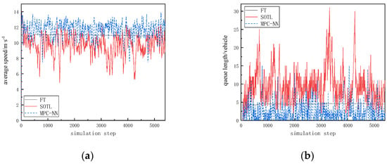
Figure 7.
Simulation results based on traffic data from the intersection of Moganshan Road and Jiaogong Road in Hangzhou. (a) The trend of average speed changes; (b) the trend of queue length changes.

Table 4.
Summary of real data in simulation experiment.
In this study, an improved graph convolutional prediction model was proposed and integrated with the deep reinforcement learning algorithm DQN into the model predictive control framework for traffic signal optimization. The experimental results indicated that, compared to traditional fixed time and actuated signal timing methods, our approach demonstrated significant advantages in reducing intersection queue lengths and increasing travel speeds. The improved graph convolutional model effectively captured the spatiotemporal features of traffic flow, enhancing the accuracy of predictions. This improved model, combined with the DQN algorithm, allowed traffic signal optimization to achieve adaptive adjustments in dynamic and complex traffic environments, thus overcoming the limitations of traditional methods in handling traffic flow fluctuations. It was shown through experimental data that our method better addressed traffic congestion issues, particularly during peak periods, exhibiting stronger robustness and flexibility. Although significant achievements were obtained in this study, several aspects still require further exploration and refinement. In the process of verifying the reliability of the model, SUMO was used to compare several common traffic signal control methods to validate the reliability of our proposed method. However, simulation software such as SUMO 1.20.0, VISSIM Demo version, and MATSim 0.10.x are based on certain assumptions made to simplify the experimental environment, while actual conditions are constantly changing. Therefore, how to set parameters that better align with real-world conditions to ensure that the experimental results are closer to reality is a topic worth discussing. Comparing the effects of control methods under the same simulation software and environment settings can to some extent reflect the superiority of our proposed method. However, deploying the control schemes into actual traffic networks to verify the practical effects of different control methods is the best approach to achieving our goal of improving traffic efficiency. This will require extensive efforts and coordination in the future.
The computational complexity of the model and its performance in real-time applications need to be optimized to facilitate deployment in larger-scale traffic networks. At the macro level, when applied to an entire city or larger transportation network, this method can theoretically still be effective but will face different challenges and considerations. Firstly, there is the issue of data integration and processing. The macro level involves larger volumes of data and requires the integration and processing of more diverse data types and sources, including data from different regions and various transportation modes. Additionally, traffic signal control at the macro level needs to consider broader factors, such as coordination between different areas, the global distribution of traffic flow, and the integration of multimodal transportation. Traffic signal control at the macro level may also require faster response times to adapt to rapidly changing traffic conditions in large-scale networks. Distributed MPC methods may be an effective approach to address this issue, which is the direction we are currently researching. Models validated at the micro level might need adjustments to accommodate the complexity at the macro level, including modifications to the model structure, parameters, and algorithms. Therefore, although optimization methods at the micro level can theoretically be applied to the macro level, further research and adjustments are necessary to ensure their effectiveness and feasibility. Moreover, traffic signal control at the macro level may need to be combined with other macro traffic management and planning tools to achieve optimal performance of the overall traffic system.
6. Conclusions
This paper combines model predictive control strategies with neural networks, leveraging the advantages of graph convolutional networks in extracting spatiotemporal correlations. Deep reinforcement learning is utilized to find optimal control strategies in different scenarios, ultimately establishing a traffic signal optimization model. Through simulation and real-world validation, the MPC-NN method demonstrates advantages over traditional fixed timing and induction-based signal control methods in improving overall traffic flow speed and reducing queue lengths. Synthetic data and real-world data are employed to simulate different traffic flow conditions, showcasing the adaptability of the MPC-NN method to diverse datasets.
MPC methods represent a dynamic optimization strategy. With the advancement of artificial intelligence technology, integrating MPC with more intelligent control methods may lead to better control effectiveness while reducing computational complexity. This constitutes a potential direction for future research.
Author Contributions
Conceptualization, D.T. and Y.D.; methodology, D.T.; writing—original draft preparation, D.T.; writing—review and editing, Y.D. All authors have read and agreed to the published version of the manuscript.
Funding
This research was funded by the International Science and Technology Cooperation Program of Henan Province, China, grant number 242102520030. This research was funded by the Foundation of Henan University of Technology for Outstanding Young Teachers, grant number 21420157.
Data Availability Statement
Data are contained within the article.
Conflicts of Interest
The authors declare no conflicts of interest. The funders had no role in the design of the study; in the collection, analyses, or interpretation of data; in the writing of the manuscript; or in the decision to publish the results.
References
- Lu, K.; Ye, Z.H.; Wu, W. Regional green wave control model for coordination path set and ring-barrier structure. China J. Highw. Transp. 2022, 35, 218–227. [Google Scholar]
- Genders, W.; Razavi, S. Asynchronous n-step Q-learning adaptive traffic signal control. J. Intell. Transp. Syst. 2019, 23, 319–331. [Google Scholar] [CrossRef]
- Hegyi, A.; Schutter, B.; Hellendoorn, H. Model predictive control for optimal coordination of ramp metering and variable speed limits. Transp. Res. Part C Emerg. Technol. 2005, 13, 185–209. [Google Scholar] [CrossRef]
- Stoilova, K.; Stoilov, T. Extensions to traffic control modeling store-and-forward. Expert Syst. Appl. 2023, 233, 120950. [Google Scholar] [CrossRef]
- Ferrara, A.; Oleari, A.N.; Sacone, S.; Siri, S. Freeways as systems of systems: A distributed model predictive control scheme. IEEE Syst. J. 2014, 9, 312–323. [Google Scholar] [CrossRef]
- Sirmatel, I.I.; Geroliminis, N. Economic model predictive control of large-scale urban road networks via perimeter control and regional route guidance. IEEE Trans. Intell. Transp. Syst. 2017, 19, 1112–1121. [Google Scholar] [CrossRef]
- Wang, Y.; Chen, H.; Yin, G.; Mo, Y.; de Boer, N.; Lv, C. Motion State Estimation of Preceding Vehicles with Packet Loss and Unknown Model Parameters. IEEE/ASME Trans. Mechatron. 2024; Early Access. [Google Scholar] [CrossRef]
- Yang, H.; Yu, W.; Zhang, G.; Du, L. Network-Wide Traffic Flow Dynamics Prediction Leveraging Macroscopic Traffic Flow Model and Deep Neural Networks. IEEE Trans. Intell. Transp. Syst. 2024, 25, 4443–4457. [Google Scholar] [CrossRef]
- Ling, J.; Lan, Y.; Huang, X. A Multi-Scale Residual Graph Convolution Network with hierarchical attention for predicting traffic flow in urban mobility. Complex Intell. Syst 2024, 10, 3305–3317. [Google Scholar] [CrossRef]
- Hu, N.; Zhang, D.F.; Xie, K.; Liang, W.; Li, K.C.; Albert, Y. Dynamic multi-scale spatial–temporal graph convolutional network for traffic flow prediction. Future Gener. Comput. Syst. 2024, 158, 323–332. [Google Scholar] [CrossRef]
- Ma, Y.J.; Chen, S.S.; Ma, Y.T. Review of convolutional neural network and its application in intelligent transportation system. J. Traffic Transp. Eng. 2021, 21, 48–71. [Google Scholar]
- Ye, B.L.; Dai, B.A.; Zhang, J.M. A survey of traffic flow prediction methods based on graph convolutional networks. J. Nanjing Univ. Inf. Sci. Technol. 2024, 3, 291–310. [Google Scholar]
- Oreshkin, B.N.; Amini, A.; Coyle, L.; Coates, M. FC-GAGA: Fully connected gated graph architecture for spatio-temporal traffic forecasting. Proc. AAAI Conf. Artif. Intell. 2021, 35, 9233–9241. [Google Scholar] [CrossRef]
- Guo, K.; Hu, Y.; Sun, Y.; Qian, S.; Gao, J.; Yin, B. Hierarchical graph convolution network for traffic forecasting. Proc. AAAI Conf. Artif. Intell. 2021, 35, 151–159. [Google Scholar] [CrossRef]
- Li, F.; Feng, J.; Yan, H. Dynamic graph convolutional recurrent network for traffic prediction: Benchmark and solution. ACM Trans. Knowl. Discov. Data 2023, 17, 1–21. [Google Scholar] [CrossRef]
- De Schutter, B.; De Moor, B. Optimal traffic light control for a single intersection. Eur. J. Control 1998, 4, 260–276. [Google Scholar] [CrossRef]
- Lin, S.; Schutter, B.; Xi, Y. Efficient network-wide model-based predictive control for urban traffic networks. Transp. Res. Part C Emerg. Technol. 2012, 24, 122–140. [Google Scholar] [CrossRef]
- Ye, B.L.; Wu, W.; Gao, H. Stochastic model predictive control for urban traffic networks. Appl. Sci. 2017, 7, 588. [Google Scholar] [CrossRef]
- Liu, X.M.; Tian, Y.L.; Tang, S.H. Short-term Traffic Flow Prediction of Multi-sections Based on Time-delay Modeling. J. Transp. Syst. Eng. Inf. Technol. 2020, 20, 54–60. [Google Scholar]
- Li, Y.; Wang, T.Z.; Xu, J.H. Traffic Demand Prediction Method Based on Deep Learning for Dynamic Traffic Assignment. J. Transp. Syst. Eng. Inf. Technol. 2024, 24, 115–123. [Google Scholar]
- Liu, Z.M.; Ye, B.L.; Zhu, Y.D. Traffic signal control method based on deep reinforcement learning. J. Zhejiang Univ. (Eng. Sci.) 2022, 56, 1249–1256. [Google Scholar]
- Ye, B.L.; Wu, W.; Ruan, K. A survey of model predictive control methods for traffic signal control. IEEE/CAA J. Autom. Sin. 2019, 6, 623–640. [Google Scholar] [CrossRef]
- Lin, S.; Schutter, B.; Xi, Y. Fast model predictive control for urban road networks via MILP. IEEE Trans. Intell. Transp. Syst. 2011, 12, 846–856. [Google Scholar] [CrossRef]
- Camponogara, E.; Oliveira, L.B. Distributed optimization for model predictive control of linear-dynamic networks. IEEE Trans. Syst. Man Cybern.-Part A Syst. Hum. 2009, 39, 1331–1338. [Google Scholar] [CrossRef]
- Pham, V.H.; Ahn, H.S. Distributed stochastic MPC traffic signal control for urban networks. IEEE Trans. Intell. Transp. Syst. 2023, 24, 8079–8096. [Google Scholar] [CrossRef]
- D’Alfonso, L.; Giannini, F.; Franzè, G.; Fedele, G.; Pupo, F.; Fortino, G. Autonomous Vehicle Platoons in Urban Road Networks: A Joint Distributed Reinforcement Learning and Model Predictive Control Approach. IEEE/CAA J. Autom. Sin. 2024, 11, 141–156. [Google Scholar] [CrossRef]
- Li, T.Y.; Wang, T.; Zhang, Y.Q. Highway Traffic Flow Prediction Model with Multi-features. J. Transp. Syst. Eng. Inf. Technol. 2021, 21, 101–111. [Google Scholar]
- Mei, X.; Fukushima, N.; Yang, B.; Wang, Z.; Takata, T.; Nagasawa, H.; Nakano, K. Reinforcement learning based traffic signal control considering the railway information in Japan. In Proceedings of the 2023 IEEE 26th International Conference on Intelligent Transportation Systems (ITSC), Bilbao, Spain, 24–28 September 2023; pp. 3533–3538. [Google Scholar]
- Han, G.; Han, Y.; Wang, H.; Ruan, T.; Li, C. Coordinated control of urban expressway integrating adjacent signalized intersections using adversarial network based reinforcement learning method. IEEE Trans. Intell. Transp. Syst. 2023, 25, 1857–1871. [Google Scholar] [CrossRef]
- Chai, H.; Zhang, H.M.; Ghosal, D.; Chuah, C.N. Dynamic traffic routing in a network with adaptive signal control. Transp. Res. Part C Emerg. Technol. 2017, 85, 64–85. [Google Scholar] [CrossRef]
- Cools, S.B.; Gershenson, C.; D’Hooghe, B. Self-organizing traffic lights: A realistic simulation. In Advances in Applied Self-Organizing Systems; Springer: Berlin/Heidelberg, Germany, 2013; pp. 45–55. [Google Scholar]
Disclaimer/Publisher’s Note: The statements, opinions and data contained in all publications are solely those of the individual author(s) and contributor(s) and not of MDPI and/or the editor(s). MDPI and/or the editor(s) disclaim responsibility for any injury to people or property resulting from any ideas, methods, instructions or products referred to in the content. |
© 2024 by the authors. Licensee MDPI, Basel, Switzerland. This article is an open access article distributed under the terms and conditions of the Creative Commons Attribution (CC BY) license (https://creativecommons.org/licenses/by/4.0/).

