Abstract
The unique structure of bearingless motors requires extra displacement sensors to monitor rotor movement, unlike conventional synchronous motors. However, this requirement inevitably escalates the cost and size of the motor. To address these issues, this paper proposes a novel approach: a bearingless synchronous reluctance motor (BSRM) without displacement sensors, utilizing the whale optimization algorithm–Elman neural network (WOA-ENN). The paper firstly introduces the suspension mechanism and mathematical model of the BSRM, upon which a function containing rotor position information is constructed. Subsequently, a sensorless method based on Elman neural network (ENN) is proposed, optimized using the whale optimization algorithm (WOA). Finally, the feasibility and reliability of the proposed approach are validated through simulations and experiments.
1. Introduction
Compared to traditional motors, bearingless motors lack bearing support and instead utilize magnetic levitation technology to suspend the rotor at the center of the stator. Consequently, bearingless motors offer several advantages, including absence of mechanical friction, elimination of the need for lubrication, prevention of leakage, high efficiency, and low noise. As a result of these benefits, bearingless motors have found successful applications in various fields, including biomedical, energy, chemical engineering, and high-precision manufacturing [1,2].
Due to their unique internal structure and lack of bearing constraints, bearingless motors experience radial displacement of the rotor. Consequently, to both ensure the normal rotation of the rotor and prevent collisions between the stator and the rotor, bearingless motors require the installation of both speed and displacement sensors. Speed sensors, typically optical encoders, are installed at one end of the shaft for accurate speed measurement, while displacement sensors are mounted within the stator to monitor radial displacement. However, the installation of mechanical sensors inevitably increases the cost and size of the motor, complicating the design and manufacturing process. Moreover, in harsh working environments such as those with high humidity, temperatures, air pollution, or dust-prone areas, installing sensors may be impractical or susceptible to strong interference, rendering them ineffective.
The aforementioned issues severely constrain the cost-effective utilization of bearingless motors in specialized applications such as aerospace, aviation, energy transport, and chemical engineering. There exists an urgent need for a rotor displacement estimation method to supplant traditional mechanical sensors, thereby simplifying the internal motor structure, reducing costs, and enhancing system reliability. The emergence of such technology holds significant importance for the widespread application and promotion of bearingless motors.
To address these challenges, several scholars have researched sensorless techniques. For instance, methods utilizing sliding mode observers (SMOs) to predict motor speed signals were proposed in [3,4]. However, the accuracy of these methods was constrained by the size and slope of their sliding mode surfaces, and as control requirements become increasingly stringent, the effectiveness of sliding mode control diminishes. In [5], the Kalman filters (KFs) were investigated, but the KFs can only be applied to linear systems. In order to apply the KFs to nonlinear systems, such as estimating the speed of a motor, it is necessary to linearize the system under study, resulting in the extended Kalman filter (EKF). However, the EKF is not very stable, and its convergence process can be slow in most cases [6].
While most methods focus on research regarding motor speed sensorless techniques, there is relatively little research on displacement sensors for bearingless motors. Reference [7] proposed a method for predicting angular velocity based on the freewheeling current of the driving phase. However, this method requires the radial displacement obtained by the displacement sensor to determine the rotor angular position. References [8,9,10] studied the high-frequency injection method (HFI), which involves superimposing a high-frequency voltage pulse on the motor’s output voltage at specific time intervals. By calculating the voltage and current at the sampling time in a two-phase stationary coordinate system or a synchronous rotating coordinate system, the estimation rotor displacement and speed estimation can be achieved. However, this method requires the motor rotor to adopt a salient pole structure, which imposes limitations. In [11], four search coils were added to a bearingless induction motor and connected to a high-frequency voltage source. The radial displacement of the rotor was then obtained by processing the midpoint voltage between the two search coils. However, the introduction of search coils occupies space in the stator slots, which can lead to a reduction in the basic performance of the motor. In [12], a method based on inductance characteristics was proposed to predict rotor displacement, but the calculation process was complex and relied on the accuracy of mathematical models. References [13,14] utilized the model reference adaptive method (MRAS) to achieve accurate prediction of rotor displacement, yet this method heavily depends on the accuracy of the model. Reference [15] utilized the variation law of dual winding magnetic flux with rotor eccentricity to design a new method for observing rotor radial displacement. However, this still relies on precise magnetic flux mathematical models, and its universality is insufficient. A neural network is an operational model comprising a large number of interconnected nodes or neurons, each representing a specific output function known as an activation function. The connections between nodes represent weighted values for the signal passing through, termed as weights, which act as the memory of an artificial neural network. Neural networks do not require specific structures or rely on precise mathematical models. They have been successfully applied in sensorless technology research [16,17]. At present, there are branches such as back-propagation neural networks (BPNNs), convolutional neural networks (CNNs), recurrent neural networks (RNNs), Elman neural networks (ENNs), and others. Among them, ENN is a type of neural network due to its local memory and feedback connection characteristics. It excels in predicting real-time data and exhibits strong computing power. In this paper, the mapping of the input and output is nonlinear because the neuron functions of ENN can be nonlinear and can handle data with temporal or sequential dependencies. This is highly suitable for the application context of this study.
However, traditional ENN applications in high-order dynamic systems often encounter issues such as slow convergence speed and susceptibility to becoming stuck in local optima [18]. To overcome these challenges, the whale optimization algorithm (WOA), inspired by the predatory behavior of humpback whales in nature, was incorporated into the neural network. This algorithm eliminates the need for manual setting of various intermediate control parameters, reducing application difficulty, improving algorithm efficiency, and increasing system response speed. It has been successfully applied in various fields, including logging curves [19], meteorological forecasting [20], and photovoltaic water pump systems [21].
Based on the above discussion, this paper designs and constructs a method based on the whale optimization algorithm–Elman neural network (WOA-ENN) to effectively predict the radial displacement of the rotor. This method not only minimizes the cost associated with sensor installation, but also eliminates the need for additional complex hardware equipment. Both the simulation and experimental results validate the feasibility and reliability of this method.
2. Basic Principle of the BSRM
To achieve stable control of the suspension force, two conditions must be satisfied: (1) the absolute difference in the number of pole pairs between the two sets of windings is 1; and (2) both sets of windings are supplied with currents of the same frequency [2]. In this paper, the torque winding of the bearingless synchronous reluctance motor (BSRM) has a pole pair number of P1 = 2, and the suspension force winding has a pole pair number of P2 = 1, with both windings supplied with currents of the same frequency. Figure 1 illustrates the principle diagram of radial suspension force generation under no-load conditions for the BSRM. The black winding Na represents the torque winding, while the red winding Nb represents the suspension winding. They are supplied with currents to produce magnetic flux Ψa and Ψb, respectively. When the current directions are as shown in Figure 1a, according to the right-hand rule, the magnetic fields formed by the two sets of windings interact, causing Ψa and Ψb to be in the same direction at gap region 3, thereby enhancing the magnetic flux density at region 3; at gap region 1, Ψa and Ψb are in opposite directions, resulting in a weakening of the magnetic flux density in this region. The imbalance in gap magnetic flux density leads to the generation of radial suspension force Fx in the opposite direction along the x-axis. Similarly, when the current directions of the two sets of windings are as shown in Figure 1b, an increase in magnetic flux density occurs at gap region 2 and a decrease occurs at region 4, resulting in the generation of radial suspension force Fy in the positive direction along the y-axis. Therefore, by controlling the magnitude and direction of the current in the suspension windings, the magnitude and direction of the radial suspension force can be effectively controlled, thereby controlling the position of the rotor [2,22].
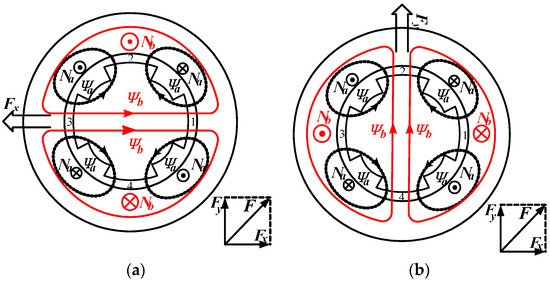
Figure 1.
Principle of radial suspension force generation. (a) x-axis direction; (b) y-axis direction.
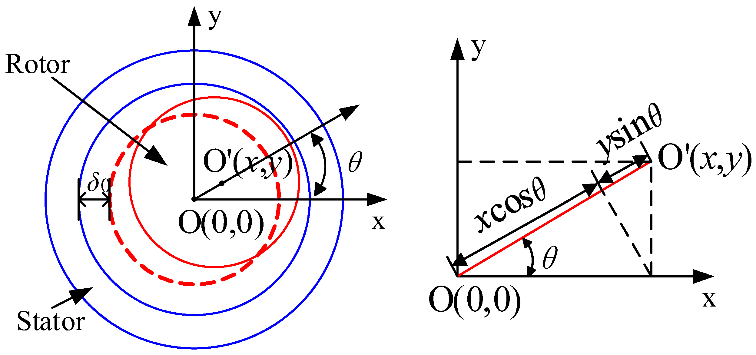
When the motor undergoes acceleration, deceleration, or sudden load changes, the rotor is inevitably affected, disrupting its original state of suspension at the center of the stator and causing radial displacement. Figure 2 illustrates the displacement of the rotor. Point O represents the original center position of the rotor without displacement, while point O’ represents the center position of the rotor after displacement. Consequently, the gap between the stator and the rotor also changes. The length of the air gap can be represented by the following equation.
where δ0 is the length of the single-sided air gap before eccentricity; θ is the angle between eccentricity and the shaft; and x and y are the displacement components of the rotor in the coordinate system, respectively.
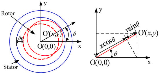
Figure 2.
Schematic diagram of the rotor displacement.
According to the mathematical derivation in [23], we can obtain the dynamic suspension motion equations of the rotor for the BSRM. The equations can be expressed as follows:
where Fx and Fy represent the controllable radial suspension forces in the x-axis and y-axis directions, respectively. Fsx and Fsy denote the Maxwell forces experienced by the rotor in the x-axis and y-axis directions, respectively. Fx0 and Fy0 represent the radial disturbance forces exerted on the rotor in the x-axis and y-axis directions, respectively. Fy0 includes the gravitational force mg acting on the rotor.
According to [2,24], Fx and Fy can be expressed as follows:
where M0 and M1 represent the mutual inductances of the two sets of windings, r is the rotor radius, l is the axial length of the rotor, μ0 = 4π × 10−7 is the air permeability, and ρ is polar arc width parameter. K is the numerical value of the fundamental wave, which is 4/π times the numerical value of the integer wave. N4 and N2 are the effective series turns per pole per phase of the torque winding and the suspension winding, respectively. The a-phase of both windings is aligned with the x-axis, and their spatial distribution follows a sinusoidal pattern. id and iq are the current components of the torque winding in the d-q rotating coordinate system, and ix and iy are the current components of the suspension winding in the d-q rotating coordinate system.
The pole arc width of the BSRM in this study is π/6; therefore, ρ = π/12. The (3) can be changed to (4).
where and , and the following equation can be obtained:
The Maxwell force in Formula (2) can be represented by the following equation:
where k is a proportionality coefficient related to the motor structure. km represents the stiffness of the suspension force displacement, which is associated with parameters such as the inherent structure of the motor, air gap magnetic flux density, core length, and air gap length. Here, based on estimation, km = 351 N/mm.
Assuming that the system sampling period is sufficiently small, discretizing the displacement terms on the right-hand side of Equation (2) yields the following equations:
where Ts is the sampling period, x(t + 1) and y(t + 1) are the displacements in the x and y directions at time t + 1, and x(t) and y(t) are the displacements in the x and y directions at time t.
By substituting Equations (5)–(7) into (2), the following equations can be obtained:
We assume that f (*) is a function related to the displacement; then, we can rewrite the above equation as follows:
It is evident that a significant correlation exists between the displacement values x and y and the currents id, iq, ix, and iy of the two sets of windings. Additionally, the currents are readily measurable. By leveraging the strong nonlinear function processing capability and adaptability of the ENN neural network, it can rapidly approximate and accurately predict target values.
Furthermore, by recursively examining the Equation (9), it can be observed that the data at each moment are intricately linked to the data from the previous moment. This inherent temporal dependency can be optimized using the WOA, which will be introduced later, facilitating rapid convergence to target values. This approximate optimization strategy enhances the response speed of the ENN and elevates the accuracy of the network, enabling it to effectively capture and predict complex relationships between variables across time intervals.
3. Elman Neural Network
Figure 3 illustrates the schematic diagram of the ENN. Standard neural networks consist of an input layer u(k), an output layer h(k), and a hidden layer q(k). In contrast, the ENN introduces an additional undertaking layer qc(k) built upon the existing hidden layer. This layer receives feedback signals from the hidden layer, with each hidden layer node connected to a corresponding node in the context layer. The role of the undertaking layer is to incorporate memory connections, allowing the previous time step’s hidden layer state to be combined with the current network input as the input to the hidden layer, effectively providing state feedback. This mechanism aids in enhancing the network’s ability to handle variables that change over time, thereby improving its robustness.
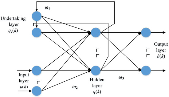
Figure 3.
Basic configuration of the ENN.
The values of ω1, ω2, and ω3 represent the weights from the undertaking layer to the hidden layer, from the input layer to the hidden layer, and from the hidden layer to the output layer, respectively. Based on experience, the values of ω1, ω2, and ω3 are 0.7, 0.15, and 0.15, respectively.
The mathematical model of the ENN is as follows:
where purelin(*) is the linear transfer function of the output neuron and tansig(*) is the tangent S-shaped function of the hidden neuron. The expression can be expressed as follows [25]:
The learning index function of the Elman neural network adopts the sum of squares function of error, representing the discrepancy between the predicted output and the actual target. The expression can be expressed as follows [19]:
where hc(k) is the target output value.
Based on the mathematical deductions in the preceding section, there exists a strong correlation between the displacement and the currents in the two sets of windings. Therefore, in this study, the input layer u(k) consists of a matrix formed by the currents id, iq, ix, and iy, while the output layer h(k) consists of a matrix formed by the displacements x and y in the x-axis and y-axis directions.
4. Whale Optimization Algorithm
The WOA was proposed by Seyedali Mirjalili in 2016, and is a new type of algorithm inspired by the predatory behavior of humpback whales in nature. Currently, it has been successfully applied in many engineering application fields.
The WOA primarily consists of three steps: surrounding the prey, bubble-net attacking, and searching for prey randomly. The detailed process is outlined as follows:
(1) Surrounding the prey: Initially, the exact position of the target prey is unknown. The WOA designates the position of the most promising individual within the existing whale group as the presumed target prey location. Subsequently, the remaining individuals in the whale group adjust their positions according to the identified location of the best candidate individual. This updating process is articulated as follows [21,26]:
where X denotes the position vector, X* represents the position vector of the best solution obtained so far, A and C are coefficient vectors, | | denotes the absolute value, · is an element-by-element multiplication, and j represents the current iteration.
It’s important to highlight that if a superior solution is discovered, the variable X must be updated in every iteration. The equation for A and C can be expressed as follows [21,26]:
where a is linearly decreased from 2 to 0 over the course of iterations; r is a random vector in [0, 1].
(2) Bubble-net attacking: During this stage, the calculation of the target prey’s position and the distance from the whale is conducted for the first time. Utilizing these data, the whale determines its most likely subsequent action. The mathematical expression governing this process is outlined below [21,26]:
where b is a constant that defines the logarithmic spiral shape and l1 is a random number between −1 and 1.
(3) Search for prey. In real-life scenarios, members of whale communities may engage in random exploration for prey positions relative to their own locations, thereby augmenting the algorithm’s capacity for global search. This behavior is represented by directing the search agent to diverge from the reference whale when the condition of is met. This aspect is mathematically characterized as follows [21,26]:
where Xrand is a random position vector (a random whale) chosen from the current population.
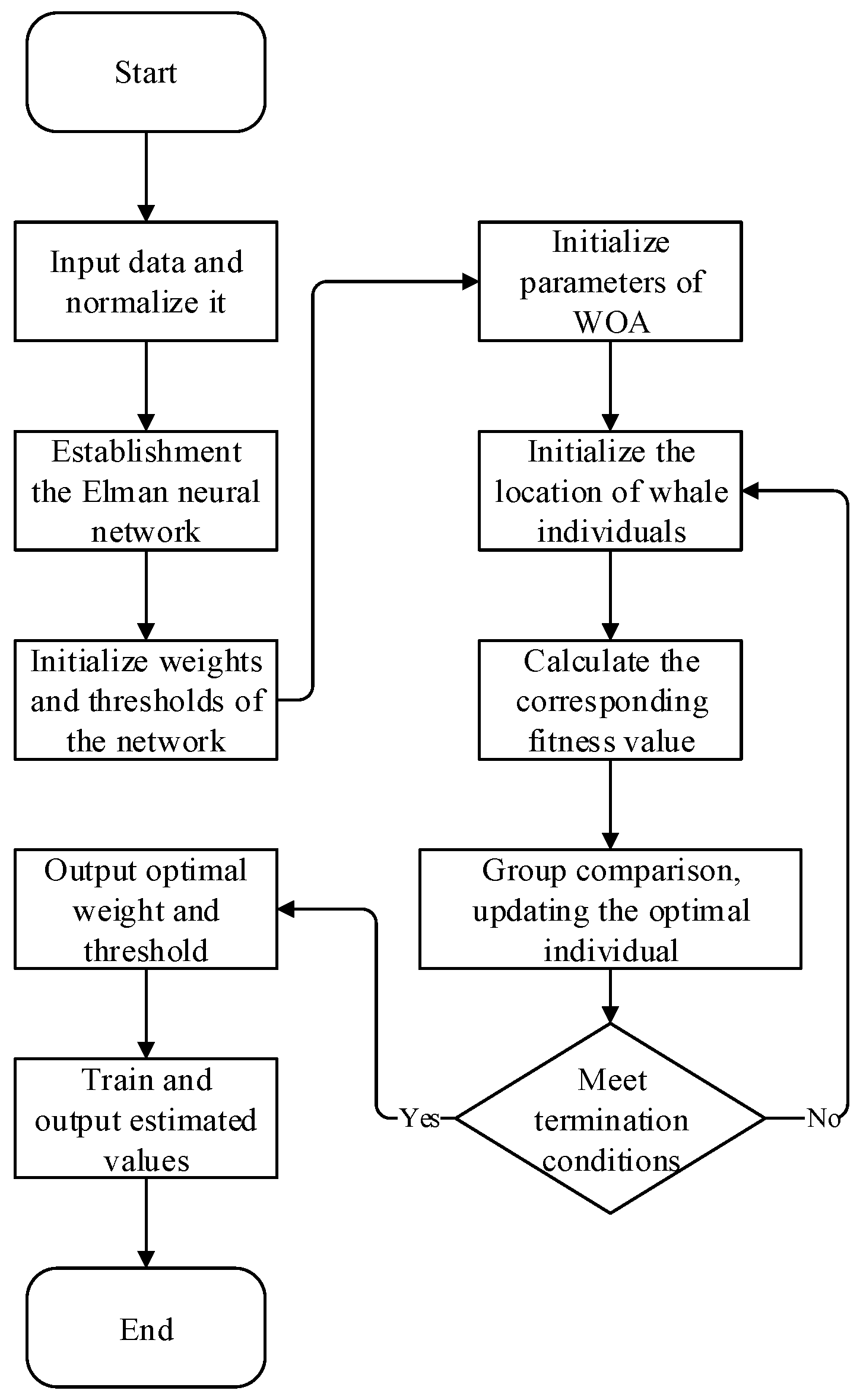
The utilization of the WOA in the ENN is illustrated in the main process depicted in Figure 4. Here is a breakdown of the process:

Figure 4.
Flowchart of the WOA-ENN.
- Step 1: Import the data and perform normalization.
- Step 2: Establish the topology of the ENN. Define variables for the input and output layers.
- Step 3: Initialize the thresholds and weights of the neural network.
- Step 4: Introduce the WOA to optimize the network. Continuously iterate using the WOA to adjust the weights and thresholds of the ENN. Repeat this process until the weights and thresholds meet the specified tolerance range. Terminate the loop at this point and proceed to the next step.
- Step 5: Update the weights and thresholds of the network based on the values provided by the algorithm.
- Step 6: Output the training set and predicted values.
It is obvious that the accuracy of both training and testing data significantly impacts the neural network’s performance. Therefore, before simulation, it is crucial to select some data to train the neural network. Displacement and current data corresponding to various time points were randomly collected. In theory, the more data, the higher the accuracy of the network. Considering the computational cost, in this paper, a sample size of 300 was chosen randomly. Among them, 100 groups were allocated for the testing set, and the remaining 200 groups were designated for the training set. In the MATLAB software R2021b environment, code was written and relevant variables were configured. The main parameters are shown in Table 1.

Table 1.
Parameters for neural networks.
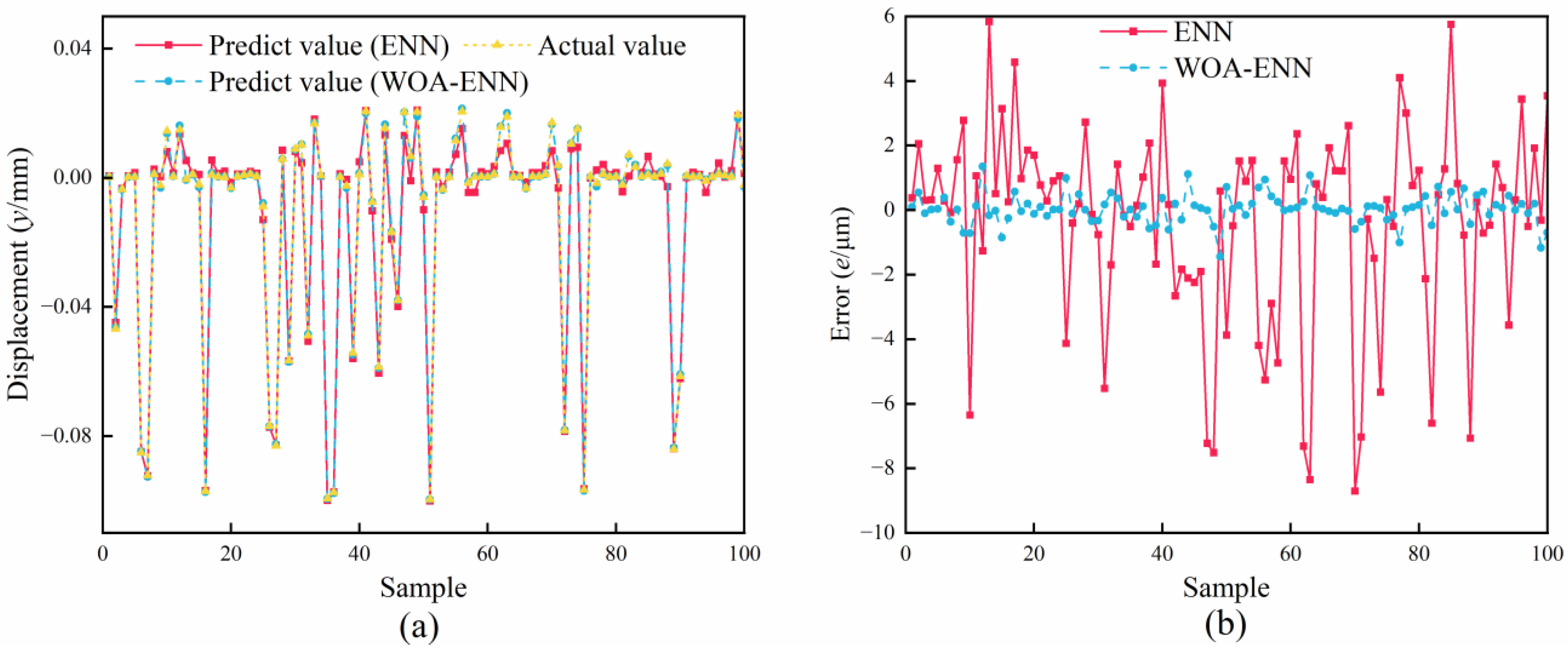
The accuracy of the neural network directly affects the credibility of subsequent research. Therefore, it is essential to validate and evaluate the trained neural network. By comparing the differences between the output values of the two networks and the actual values, the accuracy of the networks can be verified. Due to the similarity in displacement along the x-axis and y-axis directions, to reduce variables, we only select displacement along the y-axis as the output. Figure 5 illustrates the comparison of the predicted values of both networks with the actual values. Figure 5a shows the comparison between the predicted values and the actual values of the two networks, while Figure 5b displays the errors between the predicted values and the actual values for both networks. It can be observed from the figures that the predicted values of both methods are very close to the actual values, indicating high accuracy for both. However, from Figure 5b, it can be seen that the error of ENN mostly ranges from 4–8 μm, whereas the error of WOA-ENN remains within 2 μm. Clearly, the error of the latter is significantly smaller than that of the former. The results demonstrate the feasibility of the neural network and validate the precision of the WOA.

Figure 5.
Comparison of the predicted values of both networks with the actual values. (a) Result. (b) Error.
To further quantitatively analyze the differences between the two networks, evaluation indicators are introduced here, mainly including the root mean square error (RMSE), mean absolute error (MAE), determination coefficient (R2), and variance accounted for (VAF). RMSE represents the square root of the ratio of the square of the deviation between predicted and actual values to the sample size n. MAE denotes the average of the absolute errors between predicted and actual values. Smaller RMSE and MAE values indicate higher prediction accuracy of the model. R2 and VAF are commonly used to assess the linearity of the model fit. Higher values of R2 approaching 1 or VAF approaching 100% indicate better model quality. Their formulas are as follows [19,27]:
where yi represents the actual data, yi* represents the fitted data, represents the mean value, and var (*) denotes the variance function. The evaluation indicators are shown in Table 2.

Table 2.
Evaluation indicators of two models of a neural network.
Among the above evaluation indicators, R2 is a measure of the linear regression model fit. It can be graphically represented through regression analysis, as shown in Figure 6. From the graph, it can be observed that the fitting of WOA-ENN is superior.
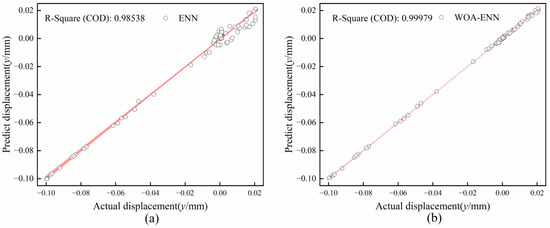
Figure 6.
Regression line plots of two networks. (a) ENN. (b) WOA-ENN.
5. Simulations and Experimental Results
In order to verify the accuracy and reliability of the method, a simulation system and experimental platform were designed and built. This paper uses a BSRM as a platform to build a displacement sensorless control strategy. The BSRM parameters are shown in Table 3.

Table 3.
Parameter of the BSRM.
5.1. Simulation Results
The trained WOA-ENN model from the previous section was integrated into the MATLAB/Simulink environment to construct a displacement sensorless simulation model for the BSRM. The control diagram is illustrated in Figure 7. The working steps of the suspension winding control system are described as follows. The current signals (id, iq, ix, iy) collected from the two windings are input into the WOA-ENN module. The predicted rotor displacement signals (x, y) obtained from the displacement sensorless technique serve as negative feedback control signals, which are compared with the desired displacement signals (x*, y*). The resulting error signals are transformed by a PID controller into suspension force signals (Fx*, Fy*). The current signals ix* and iy* of the suspension winding can be obtained through force/current conversion (Equation (3)). These signals are compared with the feedback current values ix and iy of the suspension winding. The resulting error signals are then converted by a PI controller into voltage signals, followed by Park inverse transformation and Clark inverse transformation to obtain the input voltages (u2a*, u2b*, u2c*) for the SVPWM module, thereby driving the suspension winding.
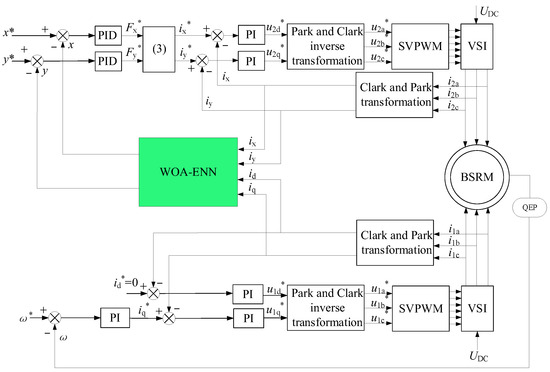
Figure 7.
Displacement sensorless control scheme of the BSRM.
For the torque winding part, a vector control method with id* = 0 is employed. The speed signal detected by the encoder serves as a negative feedback control signal, which is compared with the given speed. Subsequent processing, similar to that of the suspension winding, yields the input voltages (u1a*, u1b*, u1c*) for the SVPWM module, driving the torque winding.
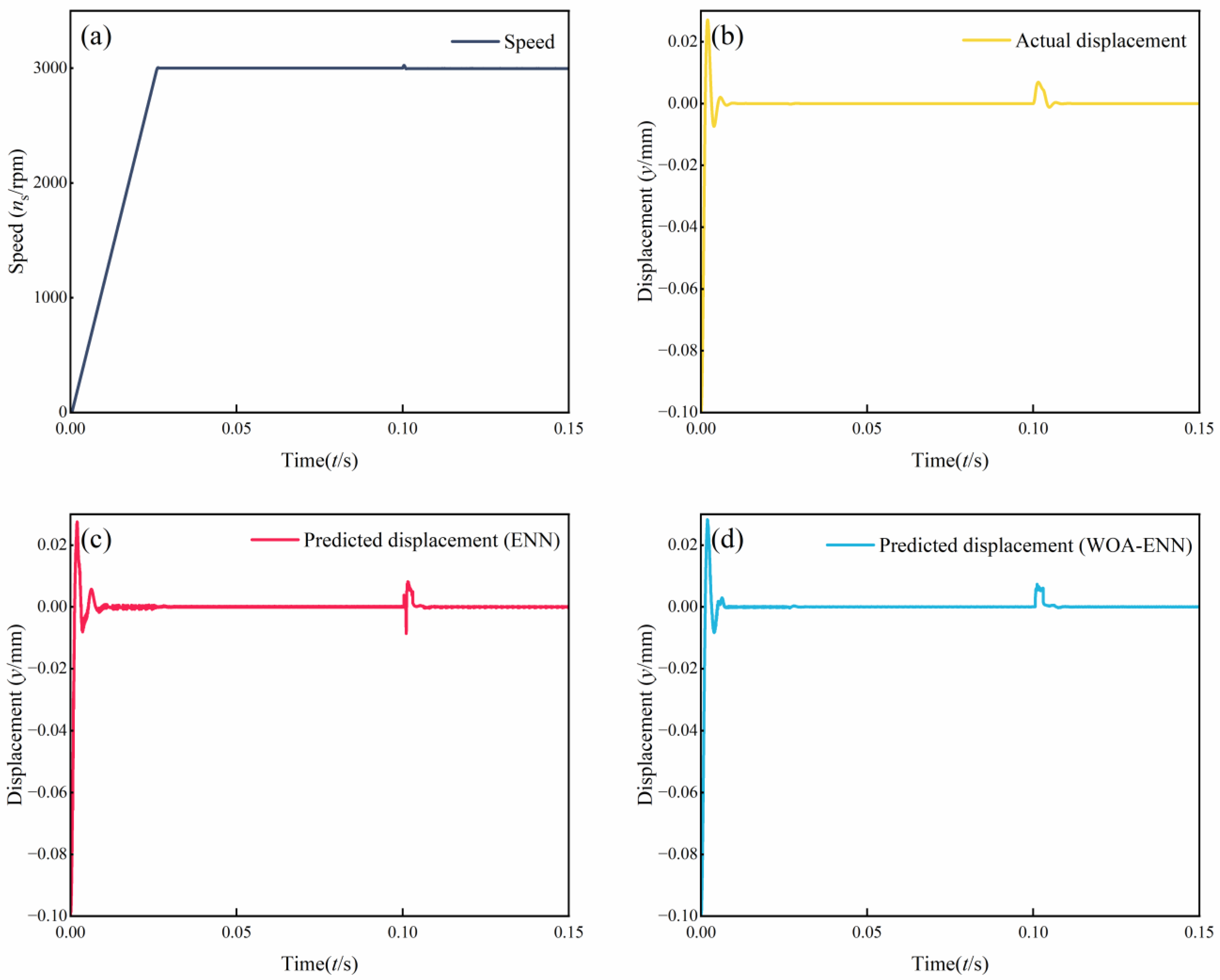
In this simulation, the variable step size odt23tb was employed as the simulation algorithm. The simulation commenced at t = 0 s and concluded at t = 0.15 s. At t = 0 s, the motor initiated operation from a standstill. By t = 0.025 s, the speed had reached 3000 r/min and remained constant until the end of the simulation. At t = 0.1 s, a disturbance of 2 Nm was abruptly applied in the positive direction of the y-axis. To showcase the superiority of the WOA, we utilized the ENN as a reference and monitored the tracking performance of the rotor displacement throughout the entire simulation duration. The entire simulation process is shown in Figure 8.
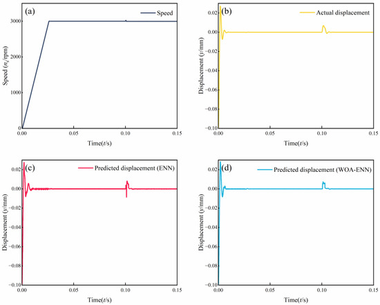
Figure 8.
Simulation results of displacement sensorless for the BSRM. (a) Speed. (b) Actual displacement. (c) Predict displacement (ENN). (d) Predict displacement (WOA-ENN).
Comparing Figure 8b–d, it can be observed that the trends of the three curves were generally consistent throughout the entire simulation process. This indicates that both the ENN and WOA-ENN methods are capable of predicting rotor displacement. However, at t = 0.1 s, there was a noticeable distortion in the ENN waveform, while the WOA-ENN waveform remained unaffected. This is attributed to the inherent limitations of ENN, such as poor convergence and robustness in handling nonlinear time series problems, whereas the latter, benefiting from the optimization of WOA, does not exhibit such pronounced deficiencies.
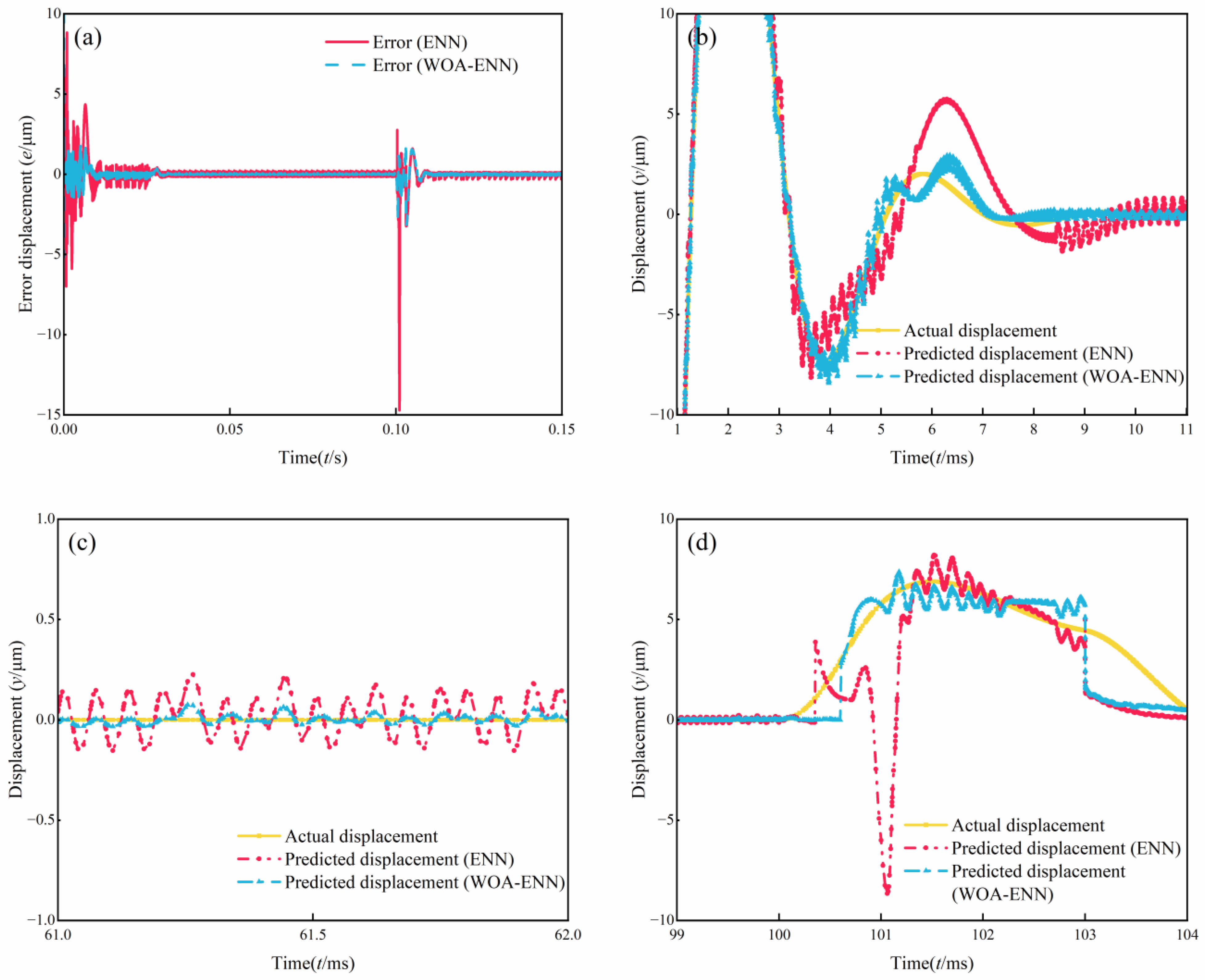
For further analysis, we compared the differences between the two methods and the actual values, as shown in Figure 9. Figure 9a shows the error results of both methods compared to the actual values throughout the entire simulation process, while the remaining three sub-figures represent zoomed-in views of the start-up phase, steady-state operation phase, and load disturbance phase of the motor, respectively. It can be observed that the fluctuation amplitude of ENN was relatively large, with errors ranging from 6 to 9 μm during the rising phase, significantly greater than the errors below 2 μm observed with the WOA-ENN method. During the steady-state operation phase of the motor, the errors of both methods were very small, but it can also be noted that the fluctuation range of the ENN method is significantly larger than that of the WOA-ENN. During the load disturbance phase, ENN produced significant errors, approximately 9 μm, indicating its inability to respond promptly to sudden load changes. In contrast, the WOA-ENN demonstrated excellent tracking performance.
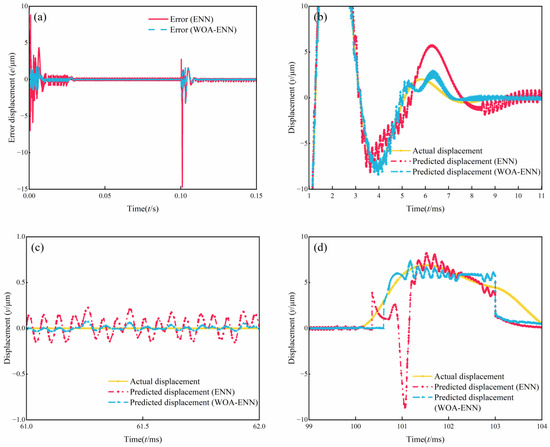
Figure 9.
Comparison of simulation of displacement sensorless for the BSRM. (a) Error. (b) Acceleration stage. (c) Smooth operation stage. (d) Load disturbance stage.
Throughout the simulation process, the WOA-ENN can accurately predict the displacement information of the rotor. Compared with traditional ENN, it has a small error and fluctuation range, proving that the proposed method is accurate, implementable, and has strong anti-interference ability.
5.2. Experimental Results
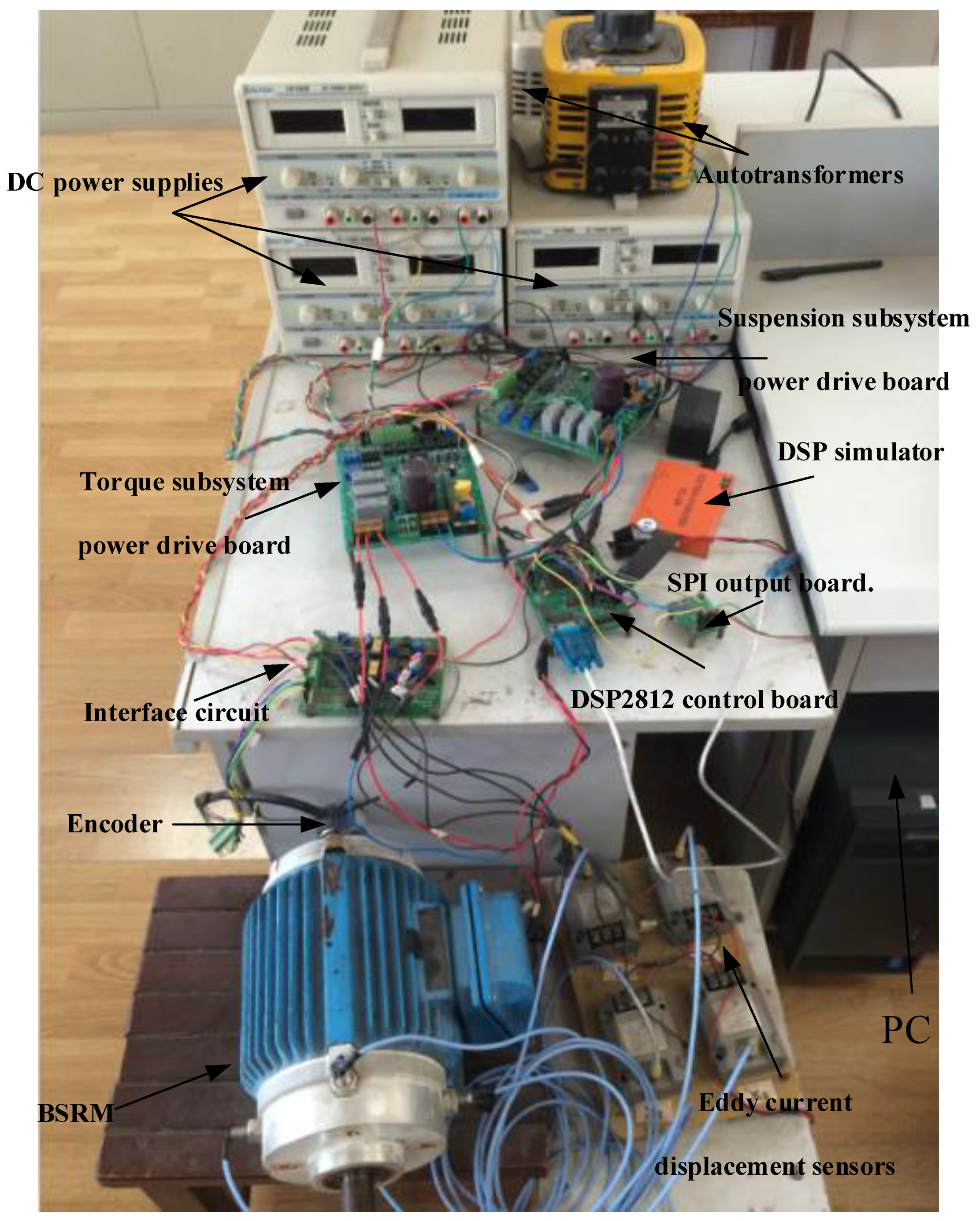
To validate the correctness of the simulation results, an experiment platform was established. The experimental parameters and simulation parameters were consistent. The BSRM experimental platform was built, as shown in Figure 10. It mainly comprised the BSRM, power drive boards, power supplies, and a DSP controller. Because the actual displacement of the BSRM could not be directly obtained, we assumed that the values measured by the displacement sensor were the true data, while the values obtained after processing by the neural network were the predicted values. The displacement sensor used in this experiment was the QH8500 model of an eddy current sensor. This type of sensor is a non-contact linear position measurement device, known for its high resolution, strong anti-interference capability, and fast response speed. An oscilloscope was used to display the displacement signal detected by the displacement sensor and the displacement signal predicted by the neural network, and they were analyzed.
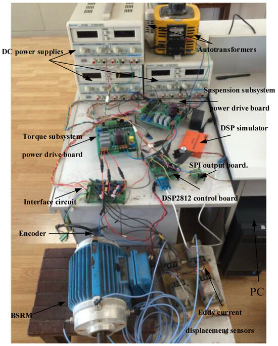
Figure 10.
Experimental platform of the BSRM.
We employed three control methods to control the suspension winding of the BSRM. The first method utilized the displacement signal detected by traditional displacement sensors as the negative feedback control signal. The other two methods, as mentioned in the Simulation Results section, used ENN and WOA-ENN to obtain the displacement signal as the negative feedback control signal. The first method served as the reference group, allowing us to demonstrate the feasibility of the proposed method and the optimization effect of the WOA.
Figure 11 shows the displacement curves of the rotor during normal motor operation. It can be observed that the fluctuations of the rotor in the x-axis and y-axis directions were relatively small, indicating the effective operation of the motor suspension control system at this time. Overall, the values measured by the sensor were the smoothest, with fluctuations within 0.5 μm, followed by the WOA-ENN with fluctuations within 1 μm and ENN with fluctuations reaching up to 4 μm. The WOA-ENN exhibited smaller fluctuations and lower errors compared to ENN, indicating its accuracy and the effectiveness of algorithm optimization.

Figure 11.
Displacement during the steady-state operation phase. (a) Actual displacement. (b) Predicted displacement (ENN). (c) Predicted displacement (WOA-ENN).
To further validate the reliability of this method, a 2 Nm load was intentionally added in the positive y-axis direction. We observed the predictive capability of this method during the load disturbance phase. Figure 12 shows the displacement comparison during this process. The values measured by the sensor were the smoothest, with fluctuations within 2 μm, followed by the WOA-ENN, with fluctuations within 4 μm, and ENN, with fluctuations reaching up to 10 μm. Comparing the three plots in Figure 12, it is evident that the sensor had the fastest response speed, with minimal fluctuations and the smoothest waveform. The performances of the two sensorless methods were not as effective as that with the sensor. However, comparing the two sensorless methods, it is evident that the WOA-ENN closely approximated the values detected by the sensor and exhibited a smaller fluctuation range. Meanwhile, the ENN’s ability to respond to sudden load disturbance was not as stable, resulting in some waveform distortion.

Figure 12.
Displacement during the load disturbance phase. (a) Actual displacement. (b) Predicted displacement (ENN). (c) Predicted displacement (WOA-ENN).
Based on the results of the simulations and experiments in this section, the WOA-ENN method was demonstrated to be feasible and accurate. However, it still faces some potential issues and challenges. The foundation of the proposed method relies on the quantity and quality of sample data. The more samples and the higher the quality, the better the performance of the method. In this study, due to workload constraints, the number of samples collected was limited. Additionally, most of the collected sample data were obtained during normal motor operation, with fewer samples collected during motor failure. Therefore, the predictive performance of the method may be compromised when the motor experiences faults. Of course, adding a certain number of fault samples can effectively improve the prediction performance.
6. Conclusions
Building upon the mathematical model proposed by previous scholars for the bearingless synchronous reluctance motor, this study extracts the relationship between the suspension winding current and the rotor radial displacement. We designed a displacement sensorless technique for the BSRM based on the WOA-ENN. The WOA was utilized to optimize the ENN, enhancing the accuracy and stability of the proposed method. Both the simulation and experimental results demonstrate the effectiveness of this approach in predicting the rotor’s radial displacement. Moreover, this method requires no additional hardware, is straightforward to implement, and exhibits strong resistance to interference. These findings underscore the promising prospects and research value of the proposed technique.
Author Contributions
Conceptualization, E.X.; methodology, E.X.; software, E.X.; validation, E.X. and R.Z.; formal analysis, E.X.; investigation, E.X.; resources, E.X.; data curation, E.X.; writing, original draft preparation, E.X.; writing—review and editing, R.Z.; visualization, R.Z.; supervision, E.X. and R.Z.; project administration, E.X.; funding acquisition, E.X. and R.Z. All authors have read and agreed to the published version of the manuscript.
Funding
This work was supported by the Open Research Subject of Key Laboratory of Fluid and Power Machinery (Xihua University), Ministry of Education (Grant No. LTDL-2023002), Project of self-made experimental instruments and equipment of Jiangsu University (Grant No. ZZYQSB202316), National Natural Science Foundation of China (Grant No. 52176038), and Key R & D projects in Jiangsu Province (Grant No. BE2021073).
Institutional Review Board Statement
Not applicable.
Data Availability Statement
All data are available in the manuscript.
Conflicts of Interest
The authors declare no conflicts of interest.
References
- Silber, S.; Amrhein, W.; Bosch, P.; Schob, R.; Barletta, N. Design Aspects of Bearingless Slice Motors. IEEE/ASME Trans. Mechatron. 2005, 10, 611–617. [Google Scholar] [CrossRef]
- Pei, T.; Li, D.; Liu, J.; Li, J.; Kong, W. Review of Bearingless Synchronous Motors: Principle and Topology. IEEE Trans. Transp. Electrif. 2022, 8, 3489–3502. [Google Scholar] [CrossRef]
- Liang, D.; Li, J.; Qu, R.; Kong, W. Adaptive Second-Order Sliding-Mode Observer for PMSM Sensorless Control Considering VSI Nonlinearity. IEEE Trans. Power Electron. 2018, 33, 8994–9004. [Google Scholar] [CrossRef]
- Li, Z.; Wang, J.; Wang, S.; Feng, S.; Zhu, Y.; Sun, H. Design of Sensorless Speed Control System for Permanent Magnet Linear Synchronous Motor Based on Fuzzy Super-Twisted Sliding Mode Observer. Electronics 2022, 11, 1394. [Google Scholar] [CrossRef]
- Bian, Y.; Yang, Z.; Sun, X.; Wang, X. Speed Sensorless Control of a Bearingless Induction Motor Based on Modified Robust Kalman Filter. J. Electr. Eng. Technol. 2023, 19, 1179–1190. [Google Scholar] [CrossRef]
- Mercorelli, P. A Two-Stage Augmented Extended Kalman Filter as an Observer for Sensorless Valve Control in Camless Internal Combustion Engines. IEEE Trans. Ind. Electron. 2012, 59, 4236–4247. [Google Scholar] [CrossRef]
- Raggl, K.; Warberger, B.; Nussbaumer, T.; Burger, S.; Kolar, J.W. Robust Angle-Sensorless Control of a PMSM Bearingless Pump. IEEE Trans. Ind. Electron. 2009, 56, 2076–2085. [Google Scholar] [CrossRef]
- Zhu, Z.Q.; Gong, L.M. Investigation of Effectiveness of Sensorless Operation in Carrier-Signal-Injection-Based Sensorless-Control Methods. IEEE Trans. Ind. Electron. 2011, 58, 3431–3439. [Google Scholar] [CrossRef]
- Ji, W.; Shi, G.; Xu, B.; Xu, J. An improved rotating HF signal injection method based on FIR filters for state estimation of BPMSM sensorless control. Adv. Mech. Eng. 2017, 9, 1–10. [Google Scholar] [CrossRef]
- Zhou, L.K.; Cao, L.; Wang, Y.; Diao, X.Y.; Zhu, H.Q. Speed Sensorless Based on High Frequency Signal Injection on Bearingless Synchronous Reluctance Motor. In Proceedings of the 31st Chinese Control Conference, Hefei, China, 25–27 July 2012; pp. 4339–4343. [Google Scholar]
- Chiba, A.; Santisteban, J.A. A PWM Harmonics Elimination Method in Simultaneous Estimation of Magnetic Field and Displacements in Bearingless Induction Motors. IEEE Trans. Ind. Appl. 2012, 48, 124–131. [Google Scholar] [CrossRef]
- Tera, T.; Yamauchi, Y.; Chiba, A.; Fukao, T.; Rahman, M.A. Performances of bearingless and sensorless induction motor drive based on mutual inductances and rotor displacements estimation. IEEE Trans. Ind. Electron. 2006, 53, 187–194. [Google Scholar] [CrossRef]
- Hua, Y.; Zhu, H. Rotor radial displacement sensorless control of bearingless permanent magnet synchronous motor based on MRAS and suspension force compensation. ISA Trans. 2020, 103, 306–318. [Google Scholar] [CrossRef]
- Li, K.; Ling, F.; Sun, X.; Cai, Y.; Zhao, D.; Yang, Z. Displacement sensorless control for bearingless induction motor drives based on the MRAS method. Int. J. Appl. Electromagn. Mech. 2020, 62, 787–805. [Google Scholar] [CrossRef]
- Chen, Y.; Zhou, Y. Radial Displacement Sensorless Control of Bearingless Flux-Switching Permanent Magnet Machines Based on Difference of Symmetric-Winding Flux Linkages. IEEE Trans. Ind. Electron. 2021, 68, 7793–7803. [Google Scholar] [CrossRef]
- Pasqualotto, D.; Rigon, S.; Zigliotto, M. Sensorless Speed Control of Synchronous Reluctance Motor Drives Based on Extended Kalman Filter and Neural Magnetic Model. IEEE Trans. Ind. Electron. 2023, 70, 1321–1330. [Google Scholar] [CrossRef]
- Sun, X.; Chen, L.; Yang, Z.; Zhu, H. Speed-Sensorless Vector Control of a Bearingless Induction Motor with Artificial Neural Network Inverse Speed Observer. IEEE/ASME Trans. Mechatron. 2013, 18, 1357–1366. [Google Scholar] [CrossRef]
- El-Sousy, F.F.M. Intelligent Optimal Recurrent Wavelet Elman Neural Network Control System for Permanent-Magnet Synchronous Motor Servo Drive. IEEE Trans. Ind. Inform. 2013, 9, 1986–2003. [Google Scholar] [CrossRef]
- Sun, Y.; Zhang, J.; Yu, Z.; Liu, Z.; Yin, P. WOA (Whale Optimization Algorithm) Optimizes Elman Neural Network Model to Predict Porosity Value in Well Logging Curve. Energies 2022, 15, 4456. [Google Scholar] [CrossRef]
- Gu, B.; Hu, H.; Zhao, J.; Zhang, H.; Liu, X. Short-term wind power forecasting and uncertainty analysis based on FCM–WOA–ELM–GMM. Energy Rep. 2023, 9, 807–819. [Google Scholar] [CrossRef]
- Malla, S.G.; Malla, P.; Malla, J.M.R.; Singla, R.; Choudekar, P.; Koilada, R.; Sahu, M.K. Whale Optimization Algorithm for PV Based Water Pumping System Driven by BLDC Motor Using Sliding Mode Controller. IEEE J. Emerg. Sel. Top. Power Electron. 2022, 10, 4832–4844. [Google Scholar] [CrossRef]
- Valente, G.; Papini, L.; Formentini, A.; Gerada, C.; Zanchetta, P. Radial Force Control of Multisector Permanent-Magnet Machines for Vibration Suppression. IEEE Trans. Ind. Electron. 2018, 65, 5395–5405. [Google Scholar] [CrossRef]
- Sugimoto, H.; Chiba, A. Stability Consideration of Magnetic Suspension in Two-Axis Actively Positioned Bearingless Motor with Collocation Problem. IEEE Trans. Ind. Appl. 2014, 50, 338–345. [Google Scholar] [CrossRef]
- Ooshima, M.; Chiba, A.; Rahman, M.A.; Fukao, T. An Improved Control Method of Buried-Type IPM Bearingless Motors Considering Magnetic Saturation and Magnetic Pull Variation. IEEE Trans. Energy Convers. 2004, 19, 569–575. [Google Scholar] [CrossRef]
- Ramadevi, B.; Kasi, V.R.; Bingi, K. Fractional ordering of activation functions for neural networks: A case study on Texas wind turbine. Eng. Appl. Artif. Intell. 2024, 127, 107308. [Google Scholar] [CrossRef]
- Mirjalili, S.; Lewis, A. The Whale Optimization Algorithm. Adv. Eng. Softw. 2016, 95, 51–67. [Google Scholar] [CrossRef]
- Liu, H.; Tian, H.-Q.; Liang, X.-F.; Li, Y.-F. Wind speed forecasting approach using secondary decomposition algorithm and Elman neural networks. Appl. Energy 2015, 157, 183–194. [Google Scholar] [CrossRef]
Disclaimer/Publisher’s Note: The statements, opinions and data contained in all publications are solely those of the individual author(s) and contributor(s) and not of MDPI and/or the editor(s). MDPI and/or the editor(s) disclaim responsibility for any injury to people or property resulting from any ideas, methods, instructions or products referred to in the content. |
© 2024 by the authors. Licensee MDPI, Basel, Switzerland. This article is an open access article distributed under the terms and conditions of the Creative Commons Attribution (CC BY) license (https://creativecommons.org/licenses/by/4.0/).


