State Observer-Based Conditioned Reverse-Path Method for Nonlinear System Identification

Abstract

In light of the complex behavior of vibrating structures, their reliable modeling plays a crucial role in the analysis and system design for vibration control. In this paper, the reverse-path (RP) method is revisited, further developed, and applied to modeling a nonlinear system, particularly with respect to the identification of the frequency response function for a nominal underlying linear system and the determination of the structural nonlinearities. The present approach aims to overcome the requirement for measuring all nonlinear system states all the time during operation. Especially in large-scale systems, this might be a tedious task and often practically infeasible since it would require having individual sensors assigned for each state involved in the design process. In addition, the proper placement and simultaneous operation of a large number of transducers would represent further difficulty. To overcome those issues, we have proposed state estimation in light of the observability criteria, which significantly reduces the number of required sensor elements. To this end, relying on the optimal sensor placement problem, the state estimation process reduces to the solution of Kalman filtering. On this ground, the problem of nonlinear system identification for large-scale systems can be addressed using the observer-based conditioned RP method (OBCRP) proposed in this paper. In contrast to the classical RP method, the current one can potentially handle local and distributed nonlinearities. Moreover, in addition to the state estimation and in comparison to the orthogonal RP method, a new frequency-dependent weighting is introduced in this paper, which results in superior nonlinear system identification performances. Implementation of the method is demonstrated on a multi-degree-of-freedom discretized lumped mass system, representing a substitute model of a physical counterpart used for the identification of the model parameters.

1. Introduction

The modeling of complex, large-scale vibrating structures plays a crucial role in the overall procedure of their design. This is particularly relevant for lightweight structures that are inherently prone to vibrations. As part of the overall design, special attention should be paid to vibration suppression and control. Different fields employ applications of model-based vibration control technologies: automotive, aerospace engineering, wind engineering, and many others. Model development, as an inevitable step in the overall model-based vibration control procedure, can be based on different assumptions; in practice, it is mainly based on the assumption of linear system behavior.

A typical linear active vibration control procedure for real applications consists of nonparametric/parametric modeling, model-based (or model-free) control synthesis, and finally, experimental evaluation of the closed-loop system performance. The standard modeling approach, usually implemented in industrial problems, is based on finite element analysis (FEA) in combination with model order reduction [1], yet this approach may often suffer from a mismatch between the model and the real structure, which in turn affects the performance of the control system.

On the other hand, a two-step modeling paradigm composed of a nonparametric model of the system in the time/frequency domain together with the appropriate use of system identification methods is an alternative to the FEA approach. Since this paradigm is case-dependent, it is expected to achieve a better match in modeling and consequently better control authority than the FE-based approach alone. It should be pointed out that the application of analytical and semi-analytical methods in the modeling phase is not discussed in this paper since they are mostly limited to simple geometries. Similarly, the control synthesis and experimental evaluation of the closed-loop system in real-time are out of the scope of this paper, and interested readers may refer to [2,3].

In order to generalize the aforementioned two-step modeling paradigm to nonlinear systems and their model-based control, several approaches are proposed in the literature based on polynomial nonlinear state space (PNLSS) system identification [4] and its further variants [5,6,7,8,9].

In this paper, we propose and implement a methodology based on the two-step modeling paradigm: the design of an underlying linear model (ULM) from system identification, augmented by incorporating a nonlinear dynamics representation aimed at generalization to a nonlinear setting. The following section represents an overview of the steps in the proposed methodology and outlines the contributions with respect to previous approaches.

2. Methodology Outline and Contributions

This section presents an outline of the generalized methodology proposed in this paper for nonlinear systems modeling based on the two-step paradigm. The methodology employs a partly known model structure based on particular case-dependent system physics and the identification of system parameters. The implementation of the general approach outlined in this section and detailed in the subsequent sections is demonstrated on a substitute model of a multi-degree-of-freedom discretized system, representing the counterpart of a physical system with nonlinear properties used for identification purposes.

In the context of the proposed methodology, first the ULM is acquired using grey-box system identification in the frequency domain, where the model states are brought into modal displacement/velocity coordinates. An important constraint in this phase is to keep the excitation level small enough such that the nonlinearities within the structure are not invoked. Since this requirement over the excitation level is a non-trivial task in the experimental situation, we propose using the multi-input/multi-output (MIMO) robust Local Polynomial Method (LPM) based on the multiple realizations of the periodic random-phase multi-sine excitation [10,11,12]. Based on the calculated contribution of the nonlinearity (through the total stochastic variance estimation) from the robust LPM, the linearity assumption of the spectral analysis can be accordingly evaluated. Additionally, sine-sweep experiments for the time–frequency analysis based on the Morlet wavelet transformation are employed to validate our observation from the LPM and examine the smoothness of potential nonlinearity in terms of system states. The interested reader may refer to [13] for the theoretical discussion; furthermore, its application in physical systems is reported in [14,15].

One should note that the direct use of the conventional $H_1$ and $H_2$ methods (see [16] regarding the experimental modal analysis) for a nonlinear system at high excitation levels will result in a distorted estimation of the frequency response functions (FRFs). These methods calculate the modal parameters based on the assumption of an uncorrelated noise contribution. This assumption is subjected to evaluation in the scope of the conditioned version of $H_1$ and $H_2$ in the RP method (also referred to as $H_{c1}$ and $H_{c2}$ in the literature [17]).

Next, the subspace system identification approach is used to parameterize the linear FRFs in the form of continuous and discrete state space systems [18]. This linear model is the basis for designing a state estimation mechanism that would capture the system dynamics later, even in the presence of nonlinearity. This extension is the gateway for moving from the linear model set to a nonlinear one.

The RP method, as part of the focus of this paper, is revisited since it can accommodate the contribution of nonlinearity in extracting the modal parameters of the nonlinear system, while the FRFs of the system obtained from $H_1$ and $H_2$ are severely distorted. Mathematically speaking, the RP method works on retrogressive input/output calculations, where for an analytical nonlinear ordinary differential equation of motion, first the spectra of the system states, the input, and outputs are calculated. Then, the input is reconstructed backward from these transformed signals. Alternative fundamental approaches are also proposed in the literature [19,20,21,22,23,24].

Richards and Singh [17] pointed out one of the main drawbacks of the RP method, which requires knowledge of the nonlinear function. However, since then, the literature has become enriched with methods for characterizing nonlinearity in terms of system states. A comprehensive explanation of this line of characterization methods is wisely reviewed in [25,26]. For instance, in a local sense, the restoring force method (also called the acceleration surface method (ASM)), initially proposed by Masri and Caughey [27] and later brought to attention by Worden [28], predicts the parameterless curve of nonlinearity by using sensor elements around the predicted nonlinearity location. The application of this approach is extensively reported in practice, e.g., [29].

On the other hand, in distributed nonlinearities such as geometrical ones due to higher-order strain terms (e.g., quadratic, cubic terms), characterization of the nonlinear function in terms of the modal displacement (stiffness) and modal velocity (damping) is tackled by analytical and experimental modeling [23,30]. As long as the characterization step is performed in a local and distributed sense, the parameterization of the nonlinearity falls within the scope of the CRP and orthogonal RP (ORP) methods. It should be noted that, based on the preliminary results from the ASM and semi-/analytical modeling methods, the proposed technique in this paper does not necessarily require measurements from the sensors around the nonlinearity. This is explained in the course of the paper. However, in short, several pairs of individual reconstructed system states (indicating a DoF in the semi-physical domain) are involved in the detection process of any nonlinear interaction. Finally, following the observer-based conditioned RP (OBCRP) method proposed in this paper, a significant reduction in the number of sensor elements is achieved. This reduction directly alleviates the issues that may arise due to the change in structural mass distribution caused by the addition of several accelerometers required by the CRP/ORP method, not to mention the requirement for costly data acquisition (DAQ) devices for post-processing analog signals.

The relevance of the proposed OBCRP method in the active control of nonlinear structures lies in the model that is available during the state/output feedback control synthesis process. In this regard, unlike the robust control methods, i.e., the multi-objective classical $H_{\infty }$ controller and $\mu$-synthesis [31], where the controller guarantees the stability of the closed-loop system based on the worst-case analysis, the generated model in this paper can serve as a less conservative alternative. In other words, instead of sacrificing the performance of the system for robustness in the presence of large modeling uncertainties, by bringing the nonlinearity into the system model, the nonlinear controller is invoked only when the nonlinearity in the system response starts to appear. It should be noted that the reason for not separating the output feedback control scenario from the state feedback in nonlinear settings is due to the separation principle, which can be fulfilled under some reasonable assumptions [32]. In other words, as soon as the nonlinear model is constructed from the combination of (1) nonparametric modeling in the frequency domain, (2) grey-box linear subspace system identification, (3) state observation using Kalman filtering, (4) nonlinearity characterization from the estimated system states (with semi-physical interpretations), and (5) quantification using the OBCRP method, a state feedback control system can be designed using some of the available standard control methods, like sliding mode control or feedback linearization. This controller may then be augmented by an extended high-gain observer proposed in [32] in order to enhance the state estimation accuracy by having the nonlinearity quantified. We believe that this new closed-loop smart structure design is a promising route toward a less conservative and more practical alternative for large-scale industrial systems where the linearity assumption is not valid to a large operational extent.

In summary, the following contributions are proposed in this paper:

(1)

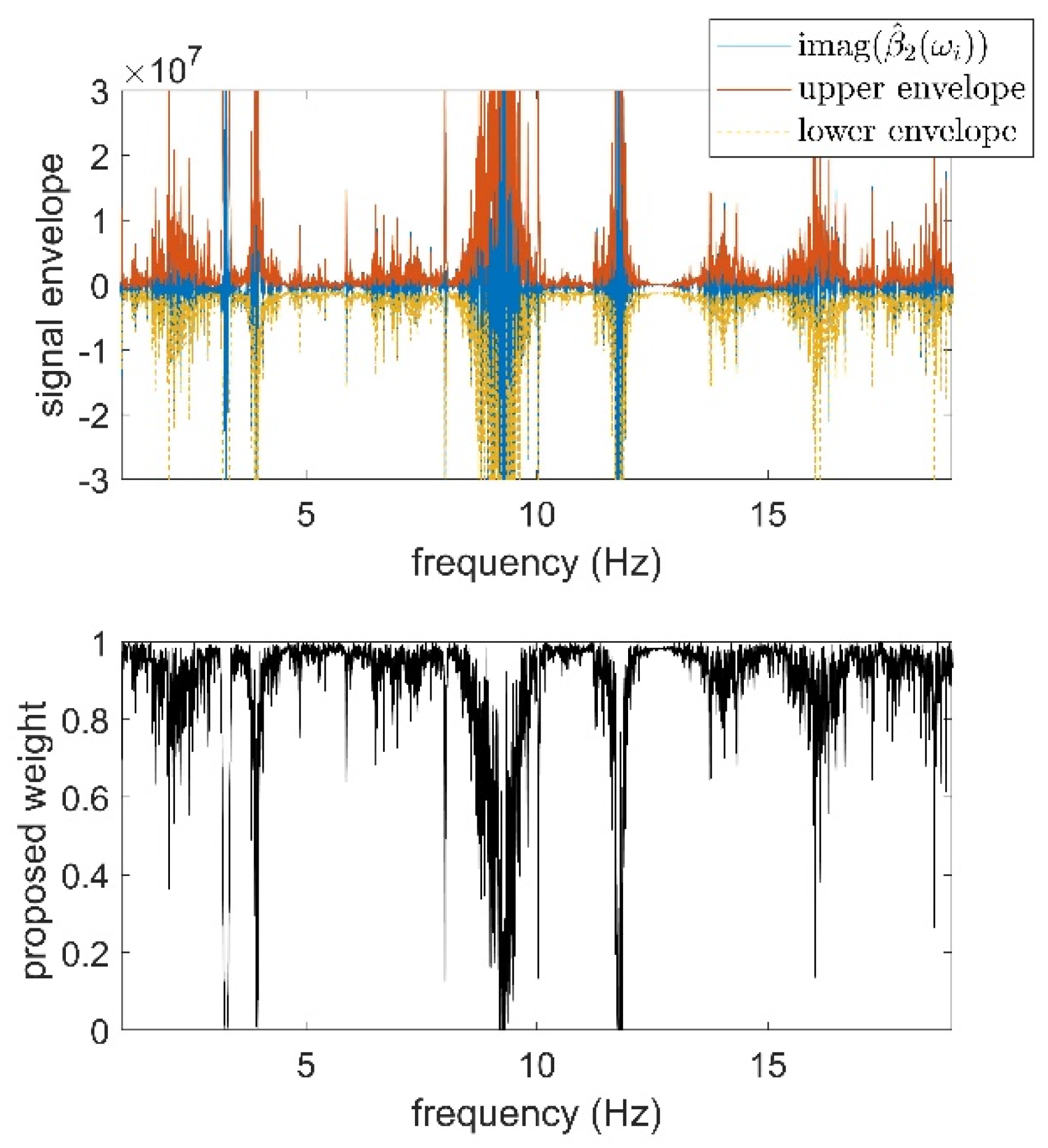
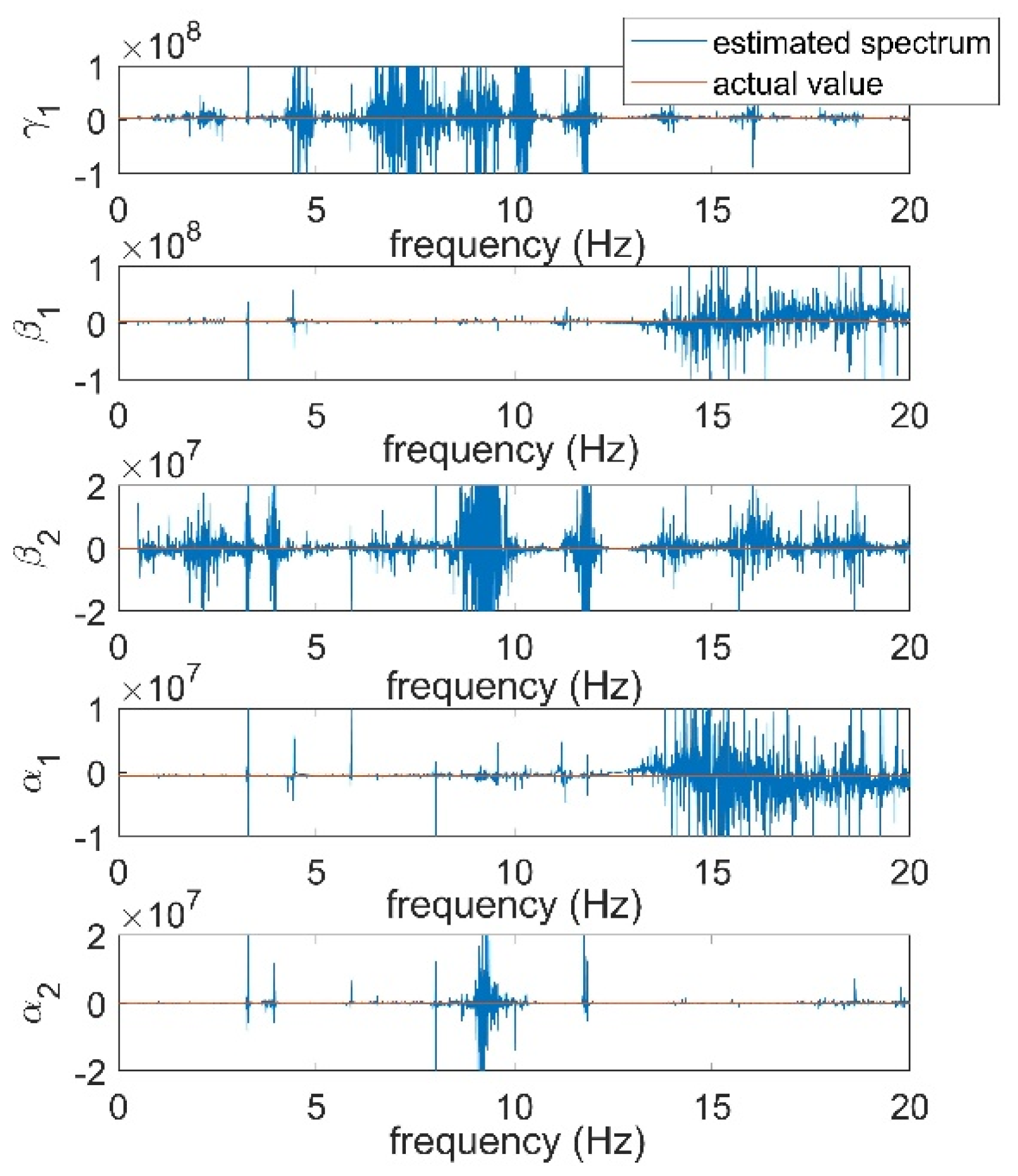
The introduction of frequency-dependent weighting in the calculation of the nonlinear coefficients in the RP method is motivated by their spectral dependencies. Accordingly, the estimations are polluted by artifacts propagated from the inaccurate estimation of the ULM, which results in a complex (non-real) estimation of the physical variables (the coefficients). The weighting proposed by Muhamad et al. [24] based on the reciprocal of the magnitude of the imaginary part of the estimated spectra is used as a background. Such weighting functions suppress the contribution of highly distorted parts of the estimated data (for the nonlinear coefficients), i.e., parts of the estimated data that have large imaginary parts. We have noticed that not only the contribution of the frequency bandwidth of the data with large imaginary parts should be suppressed in estimating these coefficients, but also a frequency window around that bandwidth should be weighted properly. Additionally, it is observed that the normalization of the frequency-dependent weighting function between zero and one is beneficial in the correct estimation of the coefficients. To this end, it is proposed to employ the normalized envelope of the imaginary part based on the Hilbert finite impulse filter as a new weighting function. It should be noted that we have abandoned the minor revision explained before on the recursive nature of the estimation of the coefficients [24] because it induces negligible improvements at the cost of the enormous computational burden for each unknown coefficient.

(2)

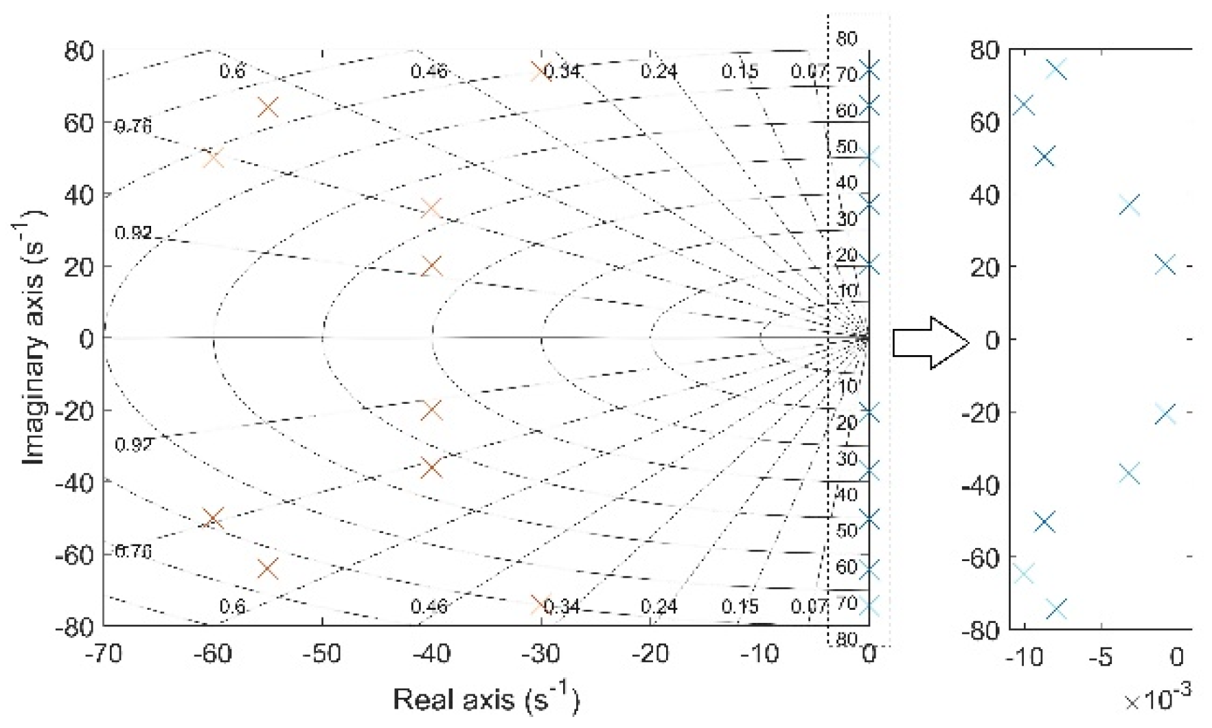
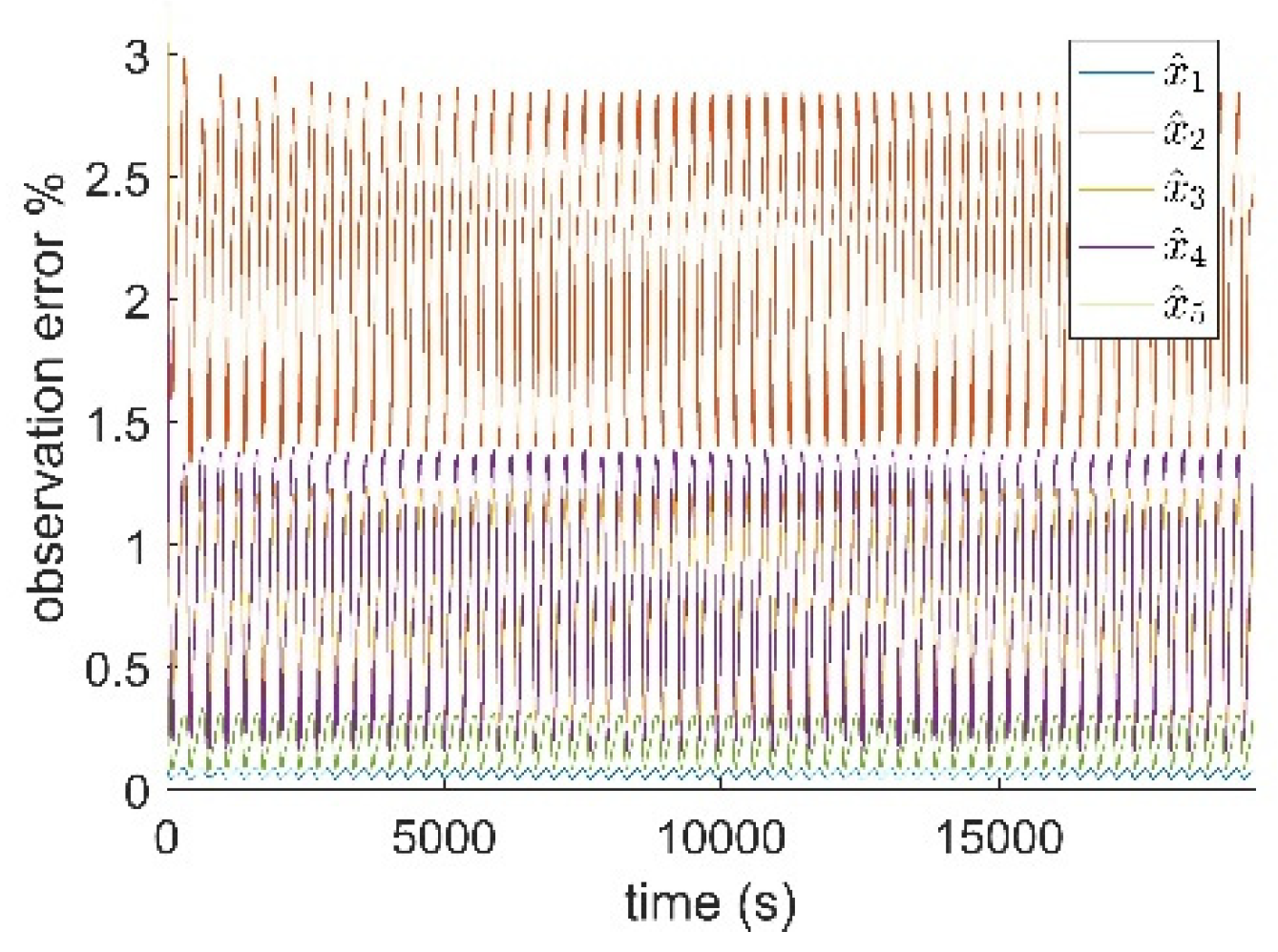
As stated previously by Worden [33], the concepts in nonlinear dynamics are often implemented for systems with low modal density, e.g., lumped parameter systems, since in practice, for large-scale continuous structures, the order of involved linear and nonlinear dynamics may be huge. Consequently, identifying appropriate measurement protocols to detect the active dynamics out of several hundred of them is a challenging task [34]. Some real-time implementations of the CRP method are tackled in the literature [23,24,35]. In this paper, based on the grey-box frequency domain linear subspace system identification, the dynamics of a continuous system is first represented in modal coordinates, which can be represented subsequently by a lumped parameter system of limited DoF for a specific operational bandwidth. The linear grey-box modeling process may result in a biased estimation of the ULM by neglecting the contribution of the unmodeled dynamics that may occur outside of the bandwidth of interest [36]. This tradeoff between the model order/model structure and the matching quality between the grey- and black-box models is discussed in detail in [37]. Then, Kalman filter state estimation is employed in order to reconstruct the system states even in nonlinear settings. It is worth mentioning that the state estimation mechanism should possess fast dynamics to accommodate the nonlinearities. Accordingly, in the formulation of the non-steady-state Kalman filtering, the contribution of the nonlinearity is addressed by considering large values for the covariance matrix associated with the process noise signal. This signal in the context of control systems can be classified as the source of matched/mismatched disturbances that invoke nonlinear behavior in the first place. Consequently, the requirement for a large number of sensors to capture a handful of states is relieved in this paper.

(3)

To address the presence of distortion in FRFs, a detection phase is performed based on the robust LPM, followed by employing the characterization results of closed-form modeling of geometrically nonlinear systems. As shown in the paper, the latter may be replaced in local nonlinearities by the ASM. This combination follows the well-known three-step paradigm for detecting, characterizing, and quantifying linearity in structural dynamics, as discussed in [25]. For this purpose, in contrast to the various forms of RP methods in the literature where the input signal is merely a Gaussian random variable, we have used single-reference random-phase multi-sine excitation. The advantages of this decision are discussed in the course of the paper. In short, it improves the estimates of the dynamic compliance functions and the coefficients of the analytically predicted (characterized) nonlinear functions. Further remarks are discussed regarding the justification of the use of spectral conditioning and the computational effort in the case of the OBCRP method. In order to highlight the sensitivity of the method in terms of measurement noise, a simulation problem is carefully designed.

The rest of the paper is organized as follows: Section 3 provides an overview of the OBCRP approach. It involves several steps, presented in detail in corresponding subsections. In addition, a concise representation of the proposed OBCRP method in the form of a ready-to-use algorithm is presented, followed by the technical definition of the random-phase multi-sine and its application in the robust LPM. The state observation problem based on non-steady-state Kalman filtering and covariance resetting in continuous and discrete form is presented subsequently in the context of the OBCRP method, with some implementation modifications based on the transition matrix approach and square root filtering. Section 4 presents the implementation results for a multi-degree-of-freedom discretized lumped mass system. Characterization of the system nonlinearity is performed based on the ASM and OBCRP procedures, and the results are documented accordingly. Final remarks and the conclusion are presented in Section 5.

3. Methodology of the Observer-Based Conditioned Reverse-Path Approach

Since in the present approach the OBCRP method is aimed at vibration control of dynamic systems, a nonlinear governing equation of motion in matrix form is selected as a starting point for the grey-box model representation:

$$M\ddot{x}\left(t\right)+C\dot{x}\left(t\right)+Kx\left(t\right)+{\displaystyle \sum _{j=1}^n}{A}_j{y}_j\left(t\right)=f\left(t\right)$$

(1)

where $M\in R^{N\times N}$, $C\in R^{N\times N}$, and $K\in R^{N\times N}$ are the mass, damping, and stiffness matrices of the final lumped parameter model, respectively. The constant matrix $A_j$ encompasses the unknown coefficients of the nonlinearity. $y_j$ represents the appropriate mathematical functions describing the nonlinearity at each junction. The analytical Fourier transformation (FT) of Equation (1) results in:

$$B\left(\omega \right)X\left(\omega \right)+{\displaystyle \sum _{j=1}^n}{A}_j{Y}_j\left(\omega \right)=F\left(\omega \right),$$

(2)

where $B$ represents the unknown ULM to be extracted from the distorted frequency domain data.

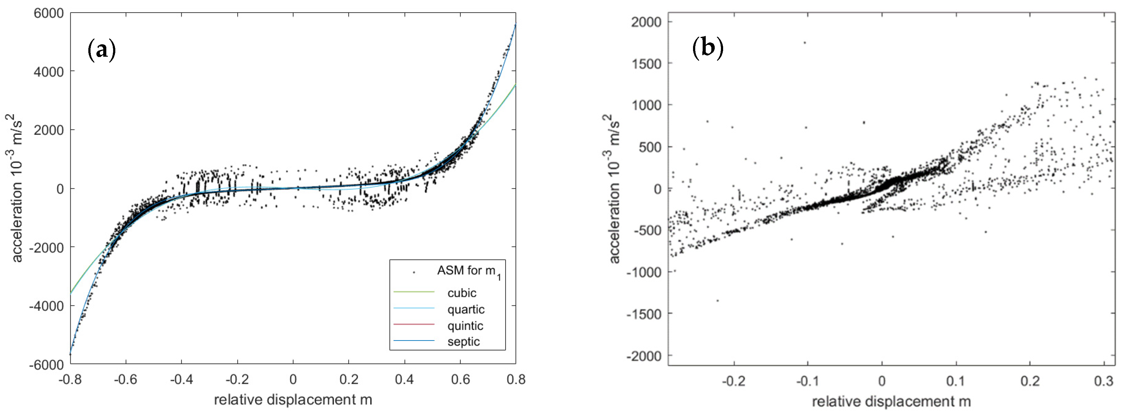
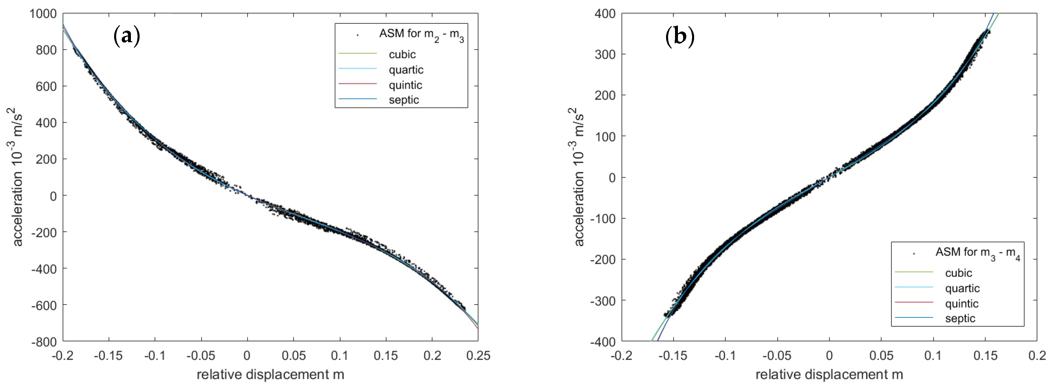
3.1. Localization and Characterization of the Nonlinearity Using the Acceleration Surface Method

Since the different variants of the RP method do not detect the local nonlinearity and do not yield the appropriate mathematical function to model the nonlinearity, the ASM is suggested. Its application allows for the determination and characterization of linear/nonlinear behavior by visualizing the relative accelerations of discrete masses in a substitute lumped mass model with respect to their displacement–velocity surface. A broader analysis of the graphical representation allows for representing the detected nonlinearity in the form of a mathematical function. Using the RP methods, the nonlinear coefficients of the mathematical function may be calculated afterwards.

The ASM represents a variant of the restoring force surface (RFS) method [38], facilitated by Newton’s second law of motion [28], applied to the discrete masses of the lumped mass model:

$${\displaystyle \sum _{n=1}^{n_p}}{m}_{i,j}{\ddot{x}}_n+g_i\left(x,\dot{x}\right)=p_i,$$

(3)

where $n_p$ is the total number of DOFs in the system; $m_{i,j}$ represents the elements of the mass matrix; $x$, $\dot{x}$, and $\ddot{x}$ are the displacement, velocity, and acceleration vectors, respectively; $g$ is the restoring force vector; and $p$ is the external force vector.

While the RFS method is generally applied to estimate the nonlinear model parameter, the ASM focuses on detecting and characterizing the local nonlinearity in the system [38]. Therefore, the term $g_i\left(x,\dot{x}\right)$ of the ASM only considers the inertia and restoring forces, which are directly related to the nonlinearity of the system, and allows for simplification of Equation (3).

$$m_{i,i}\ddot{x_i}+g_i\left(x_i-x_j,{\dot{x}}_i-{\dot{x}}_j\right)\approx p_i$$

(4)

If the masses under consideration are not excited, the force $p_i$ can be neglected in Equation (4). Since the mass has only a scaling function and does not influence the characterization of the nonlinearity, the mass in Equation (4) can also be ignored. The resulting equation of the ASM becomes:

$$g_i\left(x_i-x_j,{\dot{x}}_i-{\dot{x}}_j\right)\approx -{\ddot{x}}_i$$

(5)

Based on the fundamentals of Equation (5), the acceleration values can be plotted against the velocity and displacement values, forming a corresponding spatial surface. Cross-sections along the velocity and displacement directions are created for the nonlinear analysis. Using a graphical representation of the acceleration–displacement dependency, the smoothness of the nonlinearity is approximated by fitting the corresponding mathematical function with the appropriate order. In this paper, any damping nonlinearities associated with the observed velocity terms are neglected due to the complexity of the problem. In a subsequent step, a time–frequency analysis will be conducted to detect the range of the linear/nonlinear behavior and provide a first impression of the nonlinear behavior of the system.

3.2. Excitation Signal

In system identification, the excitation signal must fulfill the “being exciting enough” requirement. From that point of view, the multi-sine signal is the primary candidate for the single-reference excitations throughout the nonlinear parametrization process. A multi-sine signal, regardless of its phase, is a periodic time history for which the amplitude spectrum can be freely set and consequently may be represented by a Fourier series of a trigonometric sum [39]. As pointed out in [5], due to its appearance, it may be interpreted as a pseudo-random signal. However, the amplitude spectrum of a multi-sine is deterministic. The advantages of using multi-sine in nonlinear system identification in comparison to zero-mean Gaussian excitation are its periodicity, broad-band behavior with an optimizable crest factor [40], and elimination of leakage effects (after transient). In combination with [12], multi-sine excitation can be used to calculate the covariance of the noise.

The multi-sine signal is the summation of sinusoidal harmonics with arbitrary amplitudes, phases, and frequencies.

$$x\left(t\right)={\displaystyle \sum _{k=1}^{n_s}}{U}_{k}sin\left({2\pi f}_{k}t+{\phi }_k\right)$$

(6)

where $U_k$, $f_k$, and ${\phi }_k$ are the coefficients of amplitude, frequency, and phase vectors, respectively, and $n_s$ is the number of sinusoids. Using Euler’s formula and having in mind that the sinusoid can be presented as a linear combination of sine and cosine, the sinusoid of Equation (6) can be formulated as an imaginary part:

$$x\left(t\right)={\displaystyle \sum _{k=1}^{n_s}}{U}_k{e}^{\left({2\pi f}_{k}t+{\phi }_k\right)i}.$$

(7)

Using discrete Fourier transformation, Equation (7) can be presented in the form of Equation (8), where $f_k$ is substituted by the maximum frequency $f_{max}$ divided by the number of frequency components $n_s:$

$$u\left(t\right)=n_s^{-1/2}{\displaystyle \sum _{k=-n_s}^{n_s}}{U}_k{e}^{\left(2\pi k{f}_{max}t/n_s\right)i}.$$

(8)

with $U_k=U_{-k}=U\left(k\right)e^{i{\phi }_k}$. The uniformly distributed random process is realized by independent phases ${\phi }_k$ over the [0, 2π) range.

3.3. The Fast Method

The fundamental idea of this approach is to measure the nonlinear system response under the odd random-phase multi-sine excitation, where some of the in-band harmonics known as detection lines (selected randomly) are omitted. Then, the detection process is performed by examining the spectrum of the response at the detection lines, which at the same time provides an approximate estimation of the stochastic nonlinearity on neighboring lines [41]. As pointed out in [42,43], impurities in input spectra may jeopardize the estimation quality of the nonlinearity contribution since only a polluted measure of the actually implemented input signal is available. The fast method starts by grouping the excited lines, also known as the random harmonic grid. Then, the designed periodic excitation drives the nonlinear system for two or more consecutive periods, producing the steady-state response of the system. Finally, the variance of the process and measurement noise and the variance of the stochastic nonlinear distortion are calculated following Schoukens et al. [44] (pp. 200–206). This procedure is briefly explained in Figure 1.

Figure 1. Spectrum of the odd-random excitation input signal and the spectrum of the output signal with detection lines (red) and neighboring lines (green).

In Figure 1, the spectrum of the odd-random multi-sine (also random-phase) input signal where the detection lines are presented in grey color is shown on the left. Accordingly, each group includes a random selection of odd lines, which are activated within the multi-sine harmonic grid. If the system were linear, it would be expected to acquire only the excited lines (black arrows) in the spectra of the response. However, the spectrum of the unknown odd and even nonlinear distortion is detectable in the right-hand side response by red and green colored arrows, respectively. Consequently, the variance of the odd/even nonlinearities can be quantified. In contrast, the noise variance can be calculated using the non-periodic nature of the noise over repeated periods.

3.4. The Algorithm of the CRP Method

The conventional spectral analysis and coherence estimation are based on the orthogonality assumption of the normal modes, which is not satisfied in the nonlinear setting. Accordingly, the orthogonal decoupling based on the mode shapes is lost once the system possesses non-proportional damping, mode interaction, and nonlinear modes [40]. In contrast, the CRP method preserves the ease of implementation similar to classical spectral analysis to some extent. It also provides an intuitive interpretation of continuous nonlinear mechanical systems in terms of their ULM’s system states. Owing to these features, we believe the family of RP methods deserves a broader currency than they have in the literature. Technically, other than the unknowns $B$ and $A_j$, the rest of the parameters in Equation (2) are known in real-time discrete measurements using fast FT (FFT) over states and input. However, in the context of CRP/ORP methods, the states are assumed to be known. Nevertheless, due to this operation, instead of $X/Y$ in the classical notation of CRP/ORP methods, $\widehat{X}/\widehat{Y}$ are utilized, where the hat accent $\left(\widehat{.}\right)$ indicates the estimation of the associated variable since in practice only the estimation could be available. For concision purposes, the details of the CRP algorithm are not rewritten here, and the interested reader may find the description of the method in [17]. Instead, the CRP method is brought into a practically tractable form of Algorithm 1. Before presenting Algorithm 1, and for the sake of completeness, the theory behind the fourth step of the algorithm is briefly discussed. Accordingly, the spectra of the estimated states should be iteratively decoupled from the known analytical nonlinear functions’ spectra. To this end, we are interested in the calculation of the uncorrelated component of the spectra of the estimated states indicated as ${\widehat{X}}_{\left(-1:n\right)}$, which is obtained by subtracting the contribution of the spectra of uncorrelated estimated nonlinearity iteratively, i.e., ${\widehat{Y}}_{j\left(-1:j-1\right)}$ [17]:

$${\widehat{X}}_{\left(-1:n\right)}=\widehat{X}-{\displaystyle \sum _{j=1}^n}{L}_{j\widehat{X}}{\widehat{Y}}_{j\left(-1:j-1\right)}$$

(9)

where $L_{j\widehat{X}}$ is the conditioned estimate of FRF calculated as:

$$L_{j\widehat{X}}^T=G_{jj\left(-1:j-1\right)}^{-1}{G}_{j\widehat{X}\left(-1:j-1\right)},$$

(10)

while $G_{ji}$ specifies the cross-power spectral density between ${\widehat{Y}}_j$ and ${\widehat{Y}}_i$.

Algorithm 1 Summary of the CRP method

Step 1. Input excitation design: Design the input excitation signal, i.e., a Gaussian random signal or a random-phase multi-sine. Step 2. Real-time experiments and state estimation: Apply the excitation signal $f$ to the system and acquire the system output while reconstructing the system states $\widehat{x}$ as described in Appendix A. Step 3. Spectral operation: Perform spectral analysis to calculate $G_{\widehat{X}\widehat{X}}$, $G_{FF}$, $G_{F\widehat{X}}$, $G_{\widehat{X}F}$, $G_{ij}$, $G_{i\widehat{X}}$, $G_{\widehat{X}i}$, $G_{iF}$, and $G_{Fi}$ from the time–domain data of $\widehat{x}$, ${\widehat{y}}_i$, ${\widehat{y}}_j$, and $f$. (In the context of this paper, the auto-/cross-power spectral density estimates of $G_{\widehat{X}\widehat{X}},{G_{FF},G}_{F\widehat{X}}$, $G_{\widehat{X}F}$, $G_{ij}$, $G_{i\widehat{X}}$, $G_{\widehat{X}i}$, $G_{iF},\mathrm{a}\mathrm{n}\mathrm{d}{G}_{Fi}$ are calculated by employing Welch’s overlapped segment averaging estimator (see [45], pp. 910–913)). Step 4. Decorrelation step: Calculate the uncorrelated PSD of the matrices in Step 3 by following the equation for all $r=1,..,n$ iteratively: $$G_{pq\left(-1:r\right)}=G_{pq}-{\displaystyle \sum _{k=1}^r}{G}_{pk\left(-1:k-1\right)}{G}_{kk\left(-1:k-1\right)}^{-1}{G}_{kq\left(-1:k-1\right)},$$ where $p$ and $q$ are replaced with $\widehat{X}$, $F$, ${\widehat{Y}}_j$, and ${\widehat{Y}}_i$. Step 5. Condition spectral estimation of FRFs: Calculate $H_{c1}$ and $H_{c2}$ as $${H^T\left(\omega \right):H}_{c1}=G_{FF\left(-1:n\right)}^{-1}{G}_{FX\left(-1:n\right)},$$ $${H^T\left(\omega \right):H}_{c2}=G_{XF\left(-1:n\right)}^{-1}{G}_{XX\left(-1:n\right)},$$ based on the decorrelation process of Step 4. Step 6. Spectral estimation of nonlinear coefficients: Since the forcing matrix in Equation (1) is not fully populated (single-reference modal analysis), the iterative procedure of spectral extraction of the nonlinear coefficients is performed as follows: for $i=1\dots s$ $${\widehat{A}}_j^T\left({\omega }_i\right)H^T\left({\omega }_i\right)=G_{jj\left(-1:j-1\right)}^{-1}\left({\omega }_i\right)\left\{G_{jF\left(-1:j-1\right)}\left({\omega }_i\right)H^T\left({\omega }_i\right)-G_{jX\left(-1:j-1\right)}-{\displaystyle \sum _{k=j+1}^n}{G}_{jk\left(-1:j-1\right)}\left({\omega }_i\right){\widehat{A}}_j^T\left({\omega }_i\right)H^T\left({\omega }_i\right)\right\},$$ end assuming that $G_{ij\left(-1:0\right)}^{-1}\left({\omega }_i\right)=G_{ij}^{-1}\left({\omega }_i\right)$, obtained from Step 3, with ${\widehat{A}}_j^T\left({\omega }_i\right)$ being the frequency-dependent estimation of the constant unknown $A_j$. The iterative process of Step 6 starts from $j=n$ and works backwards to $j=1$, while in each step ($j$), the spectral estimation of ${\widehat{A}}_j^T\left({\omega }_i\right)$ of previous step ($j+1$) is used in the last summation operation of the right-hand side of the equation. Also, $s$ is the number of frequency domain samples. Step 7. Spectral mean operation: A scalar estimation of the nonlinear coefficients (${\widehat{A}}_j$) from the spectral estimation ${\widehat{A}}_j^T\left({\omega }_i\right)$ of Step 6 is calculated as: $$\widehat{\overline{\vartheta }}=\frac{{\sum }_{i=1}^{s}W\left({\omega }_i\right)\widehat{\vartheta }\left({\omega }_i\right)}{{\sum }_{i=1}^{s}W\left({\omega }_i\right)},$$ where $W\left({\omega }_i\right)$ is the spectral weighting explained in Section 3.1. and $\widehat{\vartheta }\left({\omega }_i\right)$ is the estimated values of the unknown elements of ${\widehat{A}}_j^T\left({\omega }_i\right)$.

Remark 1.

Welch’s technique has a small variance in the estimated periodogram by satisfying the wide-sense stationary assumption of the signal. This is achieved by overlapping the separated segments of the signal time series, augmented with a Hamming window.

3.5. Spectral Mean Estimation

As pointed out in [17] and shown in Step 7 of Algorithm 1, the unknown coefficients of the known analytical nonlinear functions are obtained in the frequency domain. Additionally, the coefficient spectra are severely distorted at frequencies close to a natural frequency, which significantly reduces the estimation quality. Moreover, the coefficient spectra are obtained as a complex value. The biased estimation of the coefficients can be reduced by using the weighting function $W\left({\omega }_i\right)$, and as recalled from [24], this weighting can be selected as $W_1\left({\omega }_i\right)=1/\left|imag\left(\widehat{\vartheta }\left({\omega }_i\right)\right)\right|,$ where $imag\left(.\right)$ is the imaginary part of the spectrum borrowed from MATLAB notation and $\left|.\right|$ indicates absolute value. This weighting is justified by pointing out that the imaginary part of the estimation spectrum must be set to zero due to a lack of physical sense. Although the improvements in the estimation performance using the weighting in [24] are undeniable, we have observed that if the bandwidth of interest encompasses several close natural frequencies, the fluctuations of the imaginary part can be high and wide-band. Additionally, if the imaginary part of the estimated spectra is zero for some frequencies, then $W_1\left({\omega }_i\right)$ is undefined. Consequently, not only the data around the natural frequencies are unreliable in the estimation, but also a wider frequency range should be weighted. More importantly, if the oscillation of the imaginary part is so high that it passes the zero axis, then the calculated mean value based on $W_1\left({\omega }_i\right)$ is wrongly weighted (in addition to the problem of one over zero). In order to solve this issue, we propose using an alternative weighting obtained from Algorithm 2.

Algorithm 2 Enhanced weighting procedure

Step 1. Signal envelope: Calculate the analytic signal for the imaginary part of the estimation spectrum of $\widehat{\vartheta }\left({\omega }_i\right)$. This operation is performed by filtering $imag\left(\widehat{\vartheta }\right)$ with the use of a Hilbert finite impulse filter. Then, the envelope is obtained from the magnitude of the analytical signal. Step 2. Detrending the calculated envelope: Bring the calculated envelope to the positive amplitude range to prevent any wrong weighting. This operation can be easily performed by adding the absolute value of the minimum of the envelope to the envelope itself. Step 3. Envelope normalization: Because of Step 2 of Algorithm 2, the problem of zero-passing in [24] will be solved. However, wide-band distortion can only be addressed if a broader band of distortion is weighted less. To this end, the detrended envelope is normalized between zero and one, referred to as $W_{nenv}\left({\omega }_i\right)$. Step 4. Weighting step: Calculate the final weighting for Step 7 of Algorithm 1 as $$W_2\left({\omega }_i\right)={\left(1-W_{nenv}\left({\omega }_i\right)\right)}^{\delta },$$ where the integer $\delta \ge 1$ is used to reduce the effect of the imaginary part even more.

4. Implementation of the OBCRP Method

The OBCRP method is implemented using the example of a multi-DoF mass–spring–damper system shown in Figure 2. The system consists of five masses $m_i$ connected with stiffness elements $k_i$ and damping elements $c_i$, where index $i=1,\dots ,5$ serves as a placeholder for the number of each component, which denotes the location in the system. Nonlinear stiffness elements are added for the nonlinear description of the system.

Figure 2. A substitute lumped mass discrete model with multi-degree-of-freedom.

In this example, the total DoF is $N=5$. $\ddot{x}\left(t\right)$, $\dot{x}\left(t\right)$, and $x\left(t\right)$ are the acceleration, velocity, and displacement vectors of the masses, respectively. As shown in Figure 2, only mass $m_1$ is excited, and the exciting vector $f$ may not be fully populated. It is clear from the controllability criteria that having a non-fully populated input should be justifiable. In other words, if the excitation signal in the nonlinear system identification phase is unable to entreat some of the dynamics of the system in the bandwidth of interest, then it is trivial not to be able to capture the associated nonlinearities for those specific DoFs. So, the design of an appropriate excitation signal is an essential part of the ASM. System parameters are shown in Table 1.

Table 1. Parameters of the system in Figure 2.

Parameter	$m_1$	$m_2$	$m_3$	$m_4$	$m_5$
value [kg]	$228$	$90$	$209$	$218$	$230$
Parameter	$k_1$	$k_2$	$k_3$	$k_4$	$k_5$	$k_6$	$k_7$	$k_8$
value [N/m]	$\mathrm{88,418}$	$\mathrm{80,838}$	$\mathrm{142,189}$	$\mathrm{177,635}$	$\mathrm{303,036}$	$\mathrm{555,131}$	$\mathrm{139,294}$	$\mathrm{224,214}$
Parameter	$c_1$	$c_2$	$c_3$	$c_4$	$c_5$	$c_6$	$c_7$	$c_8$
value [Ns/m]	$0.1$	$0.1$	$0.2$	$0.1$	$0.1$	$0.1$	$0.2$	$0.2$
Parameter unit	${\alpha }_1$ [MN/m2]	${\alpha }_2$ [MN/m2]	${\beta }_1$ [MN/m3]	${\beta }_2$ [MN/m3]	${\gamma }_1$ [MN/m5]
value	$-0.5$	$0.1$	$3$	$-0.2$	$4$

For the application and performance of the OBCRP method, mass $m_1$ of the system is excited by a multi-sine excitation denoted as a red arrow in Figure 2. The reasons for selecting this excitation signal and the principles of multi-sine signals are explained in Section 3.2. In this example, the displacement, velocity, and acceleration of masses $m_1$ and $m_5$ are acquired as output values, which are shown as green arrows in Figure 2. Kinematical values of the masses $m_2$, $m_3$, and $m_4$, denoted as black arrows, are estimated with the Kalman filter as a part of the OBCRP method, detailed in Appendix A.

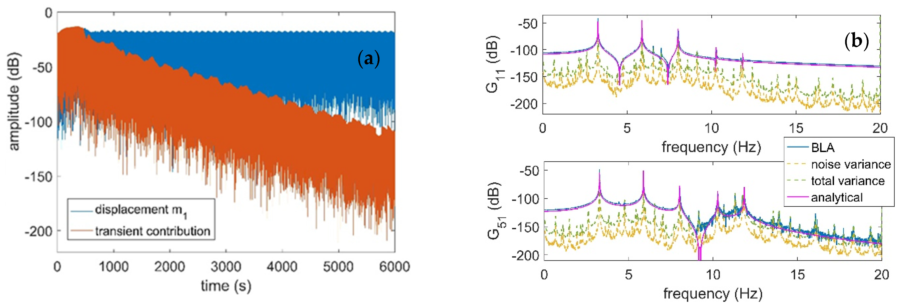
4.1. Time-Frequency Analysis

The nonlinearity detection starts with performing the time–frequency analysis based on Morlet wavelet transformation. For the mechanical system in Figure 2, the input/output data is first obtained from the single-reference excitation over $m_1$, while the measurements are collected from $m_1$ and $m_5$. Assuming that knowledge regarding the presence of nonlinearity is unavailable, two sets of simulations based on two excitation levels are performed. For this purpose, the system is excited by a chirp signal that sweeps $\left[\begin{array}{cc}0.1& 14\end{array}\right]\mathrm{H}\mathrm{z}$ at a $0.2085\mathrm{H}\mathrm{z}/\mathrm{m}\mathrm{i}\mathrm{n}$ rate. For the sake of briefness, the time history of the excitation and system response is suppressed here.

Figure 3 represents the time–frequency analysis of the system presented in Figure 2. At a lower excitation level, it can be observed that the spectrum of the output signal $\left(m_1\right)$ is almost uniform, indicating the negligible effect of the nonlinearity. Here, the result for the DoF of $m_5$ is suppressed since it does not provide additional insight into the nonlinearity behavior. However, if the operational range of the system is at a high excitation level, it is clear from the second column of Figure 3 that the nonlinearities are invoked. To make the contribution of each mode clear, the frequency response function of the ULM (black line in the left part of the figures) is augmented with wavelet-transformed data from the output. Based on the output of $m_1$ for high excitation level, three main distortions are detected at the three fundamental natural frequencies of the system. However, some shifts can be seen between the center of the distortion and the natural frequency value due to the hardening behavior. Additionally, the presence of multiple harmonics of the fundamental natural frequencies is observed by looking at the time–frequency analysis performed for output $m_1$ in dB scale for a broader frequency range of $\left[\begin{array}{cc}0& 100\end{array}\right]\mathrm{H}\mathrm{z}$. The distributed spectrum of the signal energy content in this subplot indicates energy transfer from the lower frequencies to the higher ones. It is trivial that mode interaction may happen in this case if the simulation model has natural frequencies at those high frequencies. This kind of interaction in real-time experiments is thoroughly investigated in terms of nonlinear normal modes (NNMs) by Kerschen et al. and Peeters et al. [46,47]. The presence of distortions emphasizes the necessity of using nonlinear approaches such as the OBCRP method to extract the dynamics of the system. Comparing the results of the transformed data in Figure 3 for $m_1$ and $m_5$, it can be concluded that the nonlinear contribution associated with the fundamental natural frequency propagates over the DoFs of the system; for instance, looking at the time–frequency content of $m_5$ while noting that it is not directly connected to any nonlinear function. Moreover, compared to the literature results for nonsmooth nonlinearities, e.g., SmallSat spacecraft in [48], it is clear that the nature of the nonlinearities is smooth.

Figure 3. Wavelet-transformed output signal on a non-logarithmic scale, obtained for different values of excitation amplitudes measured at different mass positions.

4.2. Implementation of the Acceleration Surface Method

Although the presence of nonlinearities and their smoothness are detected in time–frequency plots, it is difficult to interpret any spatial information from the analysis of the IO data in Figure 3. In the scope of this paper, any damping nonlinearities associated with the observed modal velocity terms are neglected due to the complexity of the problem. Assuming that the nonlinearity information is unknown, the ASM is employed to qualify the nonlinear interactions within the structure.

After solving the linear eigenvalue problem for the system in Figure 2 for the known ULM and extracting the mode shapes, it is observed that the dominant frequency range for high vibration amplitudes appears in the range of $\left[\begin{array}{cc}3.1& 4.2\end{array}\right]\mathrm{H}\mathrm{z}$. Therefore, a sine sweep excitation with an amplitude of $2500\mathrm{N}$ is applied to the structure, which is 500 s long. The resulting acceleration surface of the masses around the first junction is visualized in Figure 4.

Figure 4. Acceleration surface across the junction between the fixed base and the mass $m_1$.

The choice of excitation frequency range for the chirp signal is a process that is performed by examining the normalized eigenvectors of the ULM. The excitation frequency range should encompass the natural frequency associated with the eigenvector that induces the maximum relative displacement in the case of stiffness nonlinearity. However, some fine tuning should be performed on the excitation frequency since, due to the hardening/softening phenomena, the maximum relative displacement/velocity may shift to higher/lower frequencies, respectively. The amplitude of the excitation signal is to be selected so that the nonlinearities in the system are invoked.

A cross-section along the velocity direction is created to obtain the local nonlinear stiffness curve shown in Figure 5a. In this subplot, the relative velocity range in the ASM is limited to 0.9 m/s in magnitude. Since linear and quadratic functions cannot approximate the obtained stiffness curve, it is fitted by a cubic, a quartic, a quintic, and a septic function, as shown in Figure 5a.

Figure 5. Corresponding side-view (acceleration vs. relative displacement) of the acceleration surface used for nonparametric modeling of nonlinearity at (a) mass $m_1$ and the (b) junction between masses $m_1\mathrm{a}\mathrm{n}\mathrm{d}{m}_2$.

To determine the best-fitted function, a comparison of the coefficients of the four fitted polynomials in Figure 5a is provided in Table 2.

Table 2. Coefficients of the characterized nonlinearity for $m_1$ in Figure 2.

		Coefficients of the Polynomial in the Form of ${\mathit{p}}_1{\mathit{x}}^{\mathit{n}}+{\mathit{p}}_2{\mathit{x}}^{\mathit{n}-1}+\dots +{\mathit{p}}_{\mathit{n}+1}$						Norm of Residuals
	${\mathit{p}}_{\mathbf{1}}$	${\mathit{p}}_{\mathbf{2}}$	${\mathit{p}}_{\mathbf{3}}$	${\mathit{p}}_{\mathbf{4}}$	${\mathit{p}}_{\mathbf{5}}$	${\mathit{p}}_{\mathbf{6}}$	${\mathit{p}}_{\mathbf{7}}$
Cubic	$7835.11$	$10.21$	$-491.31$	$-3.36$	N.A.	N.A.	N.A.	$\mathrm{19,572.86}$
Quartic	$-246.31$	$7836.51$	$98.86$	$-491.79$	$-6.73$	N.A.	N.A.	$\mathrm{19,567.80}$
Quintic	$\mathrm{19,544.89}$	$118.81$	$-2198.64$	$-46.85$	$468.44$	$3.09$	N.A.	$\mathrm{13,200.854}$
Septic	$-255.75$	$\mathrm{19,537.84}$	$292.82$	$-2195.63$	$-74.79$	$468.28$	$3.71$	$\mathrm{13,200.621}$

For example, the cubic row represents the approximated stiffness curve with a cubic function of $7835.11x_1^3+10.21x_1^2-491.31x_1-3.36={\ddot{x}}_1$. $x_1$ represents the relative displacement of the mass $m_1$ towards the fixed base, and ${\ddot{x}}_1$ stands for the acceleration of mass $m_1$. It is worth mentioning that since the system in Figure 2 with the parameters in Table 1 is a so-called stiff system, the variable-step ode23tb solver in SIMULINK is selected for the simulation in this section. Table 2 is extended to the values of the norm of residuals to gain insight into the goodness of fit. The mathematical method behind the norm of residuals is based on the $L2$-Norm. Any interested reader is referred to [49].

The following observations are reportable. Comparing the norm of the residuals in Table 2, there is no improvement by increasing the polynomial order from quintic to septic. Looking at the coefficients of the polynomials for both quintic and septic, it can be observed that the coefficient of the term $x^5$ is greater than all others with some order of magnitudes, which indicates that the dominant nonlinearity is of order five nature. Additionally, comparing $p_1$ in the quintic case and $p_2$ in the septic case, it is trivial that the correct order of nonlinearity can be acceptably estimated as five.

The characterization of the nature of the interaction between $m_1$ and $m_2$ is shown in Figure 5b under the same excitation conditions and relative velocity limitations. To keep the results concise, the ASM analyses of the connection between $m_4$ and $m_5$ are suppressed since they present similar behavior as in Figure 5b.

The local nonlinear stiffness curve resulting from the junction between $m_2$ and $m_3$ is obtained by exciting the system through the input channel with a chirp signal between $\left[\begin{array}{cc}10.1& 11.3\end{array}\right]\mathrm{H}\mathrm{z}$ within a $600\mathrm{s}$ time window with an excitation amplitude of $10\mathrm{k}\mathrm{N}$. This stiffness curve of the obtained time samples for small relative velocities is shown in Figure 6a. Considering the illustrated figure and the fitted polynomial coefficients in Table 3, the following remarks are made: While noting once again that the nonlinearity is smooth, in Figure 6a, the subplot is non-symmetric. After the quadratic estimation, the other three candidates for the nonlinear function have significantly lower residuals. However, the improvement due to the additional term in the quartic function is negligible. Both the quantic and cubic estimations of the nonlinearity function preserve the non-symmetricity. The quantic form brings a four percent improvement in fitting the data. Since the nonlinearity is assumed to be unknown, performing the OBCRP method with the cubic case is recommended unless the required match in the validation phase is not met. It is correctly noted that, as highlighted in Table 3 and unlike the results in Table 2 for $m_1$, here the dominant terms are both $x^3$ and $x^2$.

Figure 6. Corresponding side-view (acceleration vs. relative displacement) of the acceleration surface used for nonparametric modeling of nonlinearity at the (a) junction between masses $m_2\mathrm{a}\mathrm{n}\mathrm{d}{m}_3$ and the (b) junction between masses $m_3$ and $m_4$.

Table 3. Coefficients of the characterized nonlinearity for the interaction between $m_2$ and $m_3$.

		Coefficients of the Polynomial in the Form of ${\mathit{p}}_{\mathbf{1}}{\mathit{x}}^{\mathit{n}}+{\mathit{p}}_{\mathbf{2}}{\mathit{x}}^{\mathit{n}-\mathbf{1}}+\dots +{\mathit{p}}_{\mathit{n}+\mathbf{1}}$					Norm of Residuals
	${\mathit{p}}_{\mathbf{1}}$	${\mathit{p}}_{\mathbf{2}}$	${\mathit{p}}_{\mathbf{3}}$	${\mathit{p}}_{\mathbf{4}}$	${\mathit{p}}_{\mathbf{5}}$	${\mathit{p}}_{\mathbf{6}}$
Quadratic	$3320.1$	$-3027.9$	$19.98$	N.A.	N.A.	N.A.	16,987
Cubic	$-\mathrm{31,985}$	$5465.4$	$-2197$	$0.0264$	N.A.	N.A.	3941
Quartic	$-\mathrm{73,26.4}$	$-\mathrm{31,354}$	$5737.2$	$-2208.4$	$-1.347$	N.A.	3921.4
Quintic	$-\mathrm{181,130}$	$\mathrm{13,366}$	$-\mathrm{23,148}$	$5126.1$	$-2284.7$	$0.87185$	3775.6

For nonparametric modeling of the nonlinear interaction between $m_3$ and $m_4$, the system is excited with a chirp between $\left[\begin{array}{cc}10.1& 11.3\end{array}\right]\mathrm{H}\mathrm{z}$ at a duration of $600\mathrm{s}$. The cross-section of the acceleration surface along the direction of the relative velocity between $m_3$ and $m_4$ is presented in Figure 6b, and for polynomial parameterizations of the data, the coefficients of the polynomial functions are sorted in Table 4.

Table 4. Coefficients of the characterized nonlinearity for the interaction between $m_3$ and $m_4$.

		Coefficients of the Polynomial in the Form of ${\mathit{p}}_{\mathbf{1}}{\mathit{x}}^{\mathit{n}}+{\mathit{p}}_{\mathbf{2}}{\mathit{x}}^{\mathit{n}-\mathbf{1}}+\dots +{\mathit{p}}_{\mathit{n}+\mathbf{1}}$					Norm of Residuals
	${\mathit{p}}_{\mathbf{1}}$	${\mathit{p}}_{\mathbf{2}}$	${\mathit{p}}_{\mathbf{3}}$	${\mathit{p}}_{\mathbf{4}}$	${\mathit{p}}_{\mathbf{5}}$	${\mathit{p}}_{\mathbf{6}}$
Quadratic	$471.53$	$1889.1$	$0.4596$	N.A.	N.A.	N.A.	7836
Cubic	$\mathrm{35,251}$	$591.45$	$1415.7$	$-0.4648$	N.A.	N.A.	2877.8
Quartic	$\mathrm{12,036}$	$\mathrm{35,308}$	$361.19$	$1415.2$	$-0.0875$	N.A.	2871.4
Quintic	$\mathrm{1,004,500}$	$\mathrm{18,729}$	$\mathrm{10,054}$	$258.14$	$1542.3$	$0.3366$	2571.6

The significant reduction in the norm of the residuals for the cubic function compared to the quadratic case and the 0.02% improvement by changing to the quartic function indicate that the cubic estimation in Figure 6b is the correct candidate. However, we have also evaluated the nonlinearity of the 5th order with a 10% lower residual. Assuming that knowledge of nonlinearity is unavailable, it is a challenging task to resolutely decide if the cubic or quintic function should be imported for the OBCRP scheme. It is certainly possible that if the recovery of the FRF after the OBCRP method for the cubic case is not satisfactory, the quantic case should be tested as well.

Consequently, in the characterization step, the localization of the nonlinearity takes place, and the analytical form of the nonlinearity for $m_1$ is quintic, while the analytical form between $m_2\mathrm{a}\mathrm{n}\mathrm{d}{m}_3$ and $m_3\mathrm{a}\mathrm{n}\mathrm{d}{m}_4$ is cubic and quadratic, respectively. The nonlinear term of Equation (1) can be concretized as:

$${\displaystyle \sum _{j=1}^{n=3}}{A}_j{y}_j=\left[\begin{array}{c}{\gamma }_1\\ 0\\ 0\\ 0\\ 0\end{array}\right]\left[x_1^5\right]+\left[\begin{array}{cc}0& 0\\ {\alpha }_1& 0\\ {-\alpha }_1& {\alpha }_2\\ 0& {-\alpha }_2\\ 0& 0\end{array}\right]\left[\begin{array}{c}{\left(x_2-x_3\right)}^2\\ {\left(x_3-x_4\right)}^2\end{array}\right]+\left[\begin{array}{cc}0& 0\\ {\beta }_1& 0\\ -{\beta }_1& {\beta }_2\\ 0& -{\beta }_2\\ 0& 0\end{array}\right]\left[\begin{array}{c}{\left(x_2-x_3\right)}^3\\ {\left(x_3-x_4\right)}^3\end{array}\right]$$

(11)

Since the mathematical function for nonlinear modeling of the system is clear, the determination of the unknown coefficients is performed using the algorithms of the CRP/OBCRB method. But therefore, the displacement, velocity, and acceleration of the $m_2$, $m_3$, and $m_4$ are needed since they are assumed to be unknown.

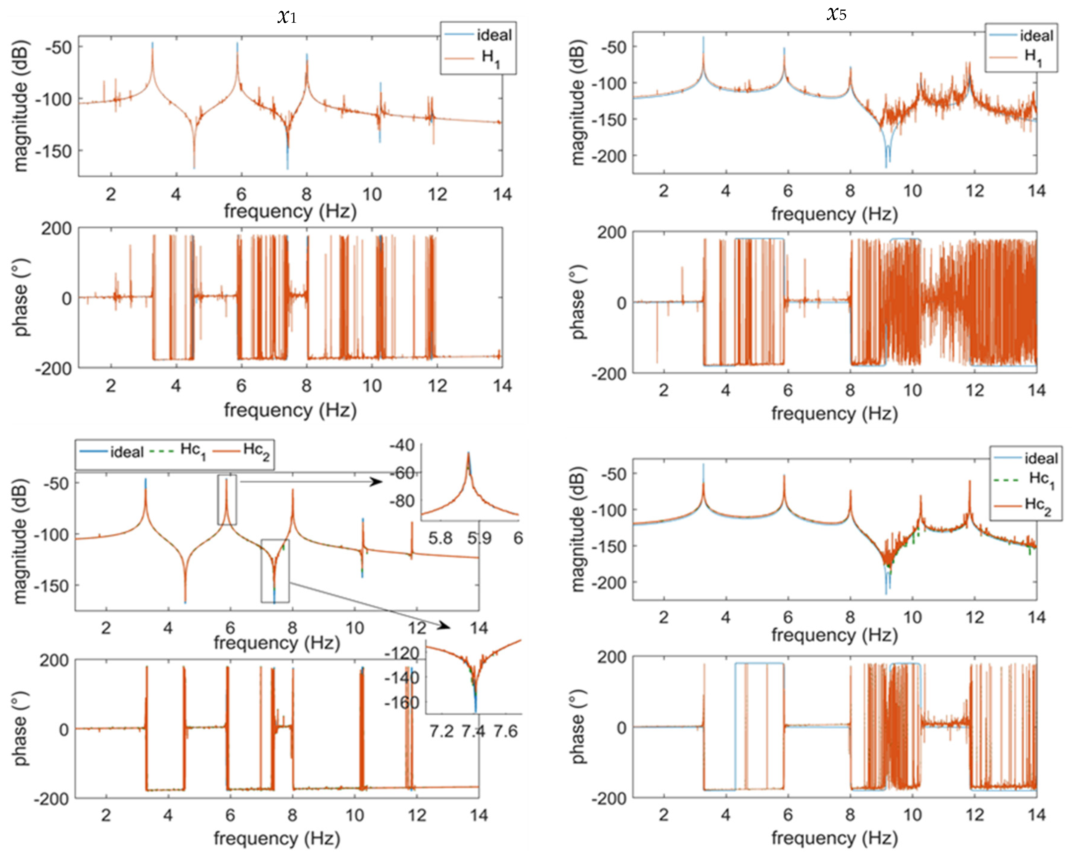
4.3. Implementation Results of the OBCRP Method

For the investigated system in Figure 2, first, the sampling time is selected as 50 µs with $2^{21}$ frequency samples, with a maximum excitation frequency of 20 Hz, and 60 periods of the random-phase multi-sine excitation are measured for seven independent realizations. The amplitude of the active lines in the frequency domain is set to 300 N. The reason for selecting such a high number for periods is the low structural damping and, consequently, the induced dominant transient noise contribution, as shown in Figure 7a.

Figure 7. (a) The transient contribution. (b) The robust LPM used to obtain the noise/nonlinearity covariance and BLA.

Using the robust LPM in [39], the total variance of the nonlinear distortion is obtained, as is the best linear approximation (BLA) of the ULM in Figure 7b. The BLA extracted from the IO data is shown in the blue line in Figure 7b. It is notable that even with the robust LPM, it is severely distorted due to the non-negligible effect of nonlinearity compared to the analytical FRF obtained from the freqresp(.) function of MATLAB. This behavior should not be mistaken for a small signal-to-noise ratio (SNR). Although this analysis provides crucial information for process noise covariance used for Kalman filter design, it fails to provide substantial insight into the nature of nonlinearity, its smoothness, and its even/odd behavior.

The Kalman filter is designed based on the obtained covariance data on process noise from the LPM, and the consequent poles of the observer at a steady state are shown in Figure 8. The results are obtained for 70 consecutive periods of the random-phase multi-sine with a crest factor of 4.0612 applied through the disturbance channel [40]. The envelope of the state observation error as a percentage is shown in Figure 9 instead of the output observation error. This representation can only be produced in the simulation example, and it is exploited to provide insight into the expected performance of the observer when estimating each displacement state separately. Consequently, the effect of observation error is expected to distort the estimation of the coefficients of analytical nonlinearities in the OBCRP method scheme as well as in the absence of measurement noise.

Figure 8. The poles of the simulation system (×) in comparison to the poles of the steady-state Kalman state observer (×).

Figure 9. The observation error in states.

Next, Algorithm 1 is applied to extract the coefficients of the characterized nonlinear functions based on the estimated states. Accordingly, employing the methodology from Appendix A, the frequency-dependent spectra of the unknown coefficients are obtained as shown in Figure 10, where the unknown variables are compared against the actual value in the simulation problem. Although the imaginary parts of the estimated spectra of the coefficients are nonzero, they are smaller by some order of magnitude than the real part. In order to pinpoint a scalar representing each coefficient, spectral mean values and weighted spectral mean values are compared following [24] and the proposed weighting in Algorithm 2. For the sake of brevity, only the weighting for the unknown coefficient of the quantic nonlinearity (${\beta }_2$) is presented here in Figure 11.

Figure 10. The real part of the estimated coefficients compared to the actual values.

Figure 11. Top: The imaginary part of the estimated spectrum of the cubic term ${\beta }_2$ and calculated envelopes. Bottom: The calculated weight based on Algorithm 2.

The estimation quality for the unknown coefficients of different weighting schemes in the spectral mean value is compared in Table 5. In this table, except for ${\gamma }_1$, the proposed weighting scheme in Algorithm 2 represents superior performance in extracting the correct value from the coefficient spectrum of the complex estimate with respect to unweighted. It should be noted that unlike the methods available in the literature, where system states are assumed to be known as a result of the generalization regarding the state estimation, the calculated scalar estimates are indeed more erroneous than those in [17,24]. This emphasizes the importance of suppressing the observation error in order to have less bias.

Table 5. Error of the estimation associated with different weighting schemes.

Coefficients	True Value	Error (%)
		Unweighted Mean	Weighted: Muhamad et al. [24]	Weighted: Present
${\alpha }_1$ ${\alpha }_2$	$-500\mathrm{k}\mathrm{N}/{\mathrm{m}}^2$	23.38	21.42	4.02
	$100\mathrm{k}\mathrm{N}/{\mathrm{m}}^2$	48.1	2.39	13.58
${\beta }_1$	$3\mathrm{M}\mathrm{N}/{\mathrm{m}}^3$	22.32	74.74	1.09
${\beta }_2$	$-0.2\mathrm{M}\mathrm{N}/{\mathrm{m}}^3$	407.22	8.96	0.79
${\gamma }_1$	$4\mathrm{M}\mathrm{N}/{\mathrm{m}}^5$	18.72	12.70	27.4

Remark 2.

It is also noted that the state estimation error covariance in standard Kalman filtering converges to zero in a short period, which limits the state observation performance in the vicinity of dynamic nonlinearities. Consequently, the results in Figure 10 and Figure 11, and Table 5 are obtained by covariance resetting every ten seconds. The idea of covariance resetting in adaptive control dates back to the fundamental works of Goodwin et al. [50]. Since then, several intelligent algorithms have also been brought into Kalman filter covariance resetting, e.g., the adaptive Kalman filter by Yu et al. [51], which mostly differs over the resetting time and resetting factor. Additionally, the adaptive fuzzy observer and intelligent algorithms augmented with a Kalman filter, which may improve the estimation performance, can significantly contribute to the quantification accuracy of the OBCRP method [2,52,53]. However, such alternations are out of the scope of this paper and will be the subject of further investigations.

Remark 3.

The Kalman gain that is updated based on the matrices of the ULM may take a long time to converge to the suboptimal solution. This solution is the trivial consequence of tuning a linear observer on a nonlinear system. In order to have faster convergence, in the results of Figure 10 and Figure 11, and Table 5, first a steady-state Kalman filter is designed, and the obtained gain is utilized to initialize the Kalman gain in a non-steady state case. This reduces the transient behavior of the filter. However, a more systematic approach to moving towards an optimal solution in the context of the extended Kalman filter would be to perform an iterative design. Accordingly, the initialization of the observer may be performed on similar lines as in this paper, followed by a correction step that may be realized by the use of a QR-factorized cubature Kalman filter (CKF) structure. The CKF operates by incorporating the higher-order derivatives of the nonlinear state equation as well as the first-order derivatives in the extended Kalman filter scheme in the design process, where the derivatives are obtained based on the identified system from the OBCRP method. The QR-factorized CKF is expected to reduce the numerical issues in the covariance matrix updating and has proven to have superior accuracy compared to the pure Kalman filter [54]. Consequently, having a lower observation error contributes to the unbiased extraction of the nonlinear coefficients following the discussion in the paragraph before Remark 2.

Finally, the ULM, based on the classical $H_1$ function, is compared with regard to the recovered conditioned FRFs using the OBCRP method, see Figure 12. The magnitude and phase are shown in Table 5 for the two outputs $x_1$ and $x_5$. As expected, the classical estimation of the FRFs based on $H_1$ is severely distorted under the effect of invoked nonlinearity. However, the conditioned spectral analysis based on the OBCRP method recovers the ULM correctly.

Figure 12. Conditioned and unconditioned FRFs in comparison to the correct linear estimate represented for selected states x₁ and x₅.

To do justice to the full performance evaluation of the OBCRP method and Algorithm 2 and simultaneously have a perception of the sensitivity of the proposed combination with respect to the measurement noise before experimental tests, the estimation process is performed in the presence of synthetic noise. To this end, the system output signals are polluted in Simulink with 1% and 3% colored Gaussian noise with the approximate frequency content shown in Figure 13a (for one realization). Two cases are compared using the polluted observed states and nonlinearity time history. The colored noise is generated by filtering a band-limited white noise with a Butterworth high-pass filter of eighth order with an edge frequency of 100 Hz, mostly the higher frequencies of the measurement output. The conditioned $H_1$ estimate ($H_{c1}$) of the ULM is compared with the analytical FRF of the system in Figure 13b for the two different noise levels.

Figure 13. (a) The frequency content of the sampled colored noise acting on the measurement outputs. (b) The extracted FRFs under the prescribed measurement noise levels in Table 6.

The comparison of nonparametric plant models representing the linear part of the system extracted based on the OBCRP method for various noise levels in Figure 13b shows that: (1) As the noise power increases, the FRFs are distorted, respectively. Consequently, in real-time experiments, contactless laser Doppler vibrometers are preferred over piezoelectric accelerometers due to the higher SNR that they can deliver. (2) Using the weighting of Algorithm 2, there is no direct connection between the noise level and the accuracy of the estimated coefficients (see Table 6).

Table 6. Error of the estimation for different measurement noise levels.

Coefficients	Error (%)
	1% Noise Power	3% Noise Power
${\alpha }_1$	11.35	11.76
${\alpha }_2$	9.77	5.80
${\beta }_1$	36.55	31.17
${\beta }_2$	32.33	7.76
${\gamma }_1$	15.04	19.34

This is an important feature in contrast with the results of [24]. It is justified by introducing steps 2 and 3 in Algorithm 2, where the effect of frequency ranges with high fluctuation rates on imaginary parts of the estimated spectrum is largely discarded. In other words, as the SNR decreases, the normalized envelope of the imaginary part (which has higher fluctuations, respectively) becomes wider, suppressing the bandwidth with additional fluctuations in comparison to the case with a better SNR. (3) The distortions in the estimated FRFs are mostly due to the observation error. In the spectral analysis involved in the OBCRP method, the effect of noise can be significantly controlled by performing averaging based on the Hamm window [39].

5. Conclusions and Outlook

The paper presents the OBCRP method as a synergy of the conditioned RP method and the state estimator, which facilitates the availability of all the system states at all times, even in cases when not all states are available for measurement or if measurement is not possible. For the representation of nonlinear systems, the underlying linear model was estimated using system identification based on the frequency response function, whereas the nonlinear part of the system model is represented in terms of polynomials of corresponding higher orders. The type and order of the nonlinearity are determined by applying the ASM. Finally, the implementation of the OBCRP method has successfully been demonstrated on the example of a lumped mass system with multi-DoF. For the conditioned spectral estimation of FRFs, a spectral operation is performed based on the state estimation and the excitation signal. In the conditioned $H_{c1}$ and $H_{c2}$ method, the nonlinear coefficients are recalculated using spectral estimation and subjected to a novel weighting proposed in the paper. In this latter process, the lost information of the imaginary part is taken into account. Further research regarding incorporating a disturbance variable into the OBCRP method is needed. The OBCRP method successfully recovers the FRFs of the ULM and parametrizes the nonlinearity of the nonlinear system. Again, it is emphasized that the method was applied only to a simulative example. The method will be investigated on an experimental test consisting of a clamped-clamped nonlinear beam with two parts of different thicknesses in the next step.

Appendix A.1. State Estimation Using Kalman Filtering

In relation to the presented discrete lumped mass model (Figure 2), since the displacement, velocity, and acceleration of the masses $m_2$, $m_3$, and $m_4$ are not accessible, an optimal estimation algorithm, the well-known Kalman filter (KF), is integrated into the OBCRP method. For the realization of a state observer, first, Equation (1) of the grey-box model is brought into state-space form by defining an auxiliary state vector $x=\left[x\dot{x}\right]$

$$\dot{x}=Ax+Bu$$

(A1)

$$y=Cz$$

(A2)

where (A1) represents the state equation and (A2) the output equation. The system matrix in the state equation can be calculated from the mass, stiffness, and damping matrix of the grey-box model as

$$A=\left[\begin{array}{cc}{0}_{5\times 5}& I_{5\times 5}\\ -M^{-1}K& -M^{-1}C\end{array}\right]$$

(A3)

with $0_{N\times N}\in R^{N\times N}$ and $I_{N\times N}\in R^{N\times N}$ being zero and identity matrices, respectively. $B$ is the input vector, and in the case of the investigated system shown in Figure 2, it is given as:

$$B={\left[\begin{array}{ccc}{0}_{1\times 5}& \frac{1}{m_1}& 0_{1\times 4}\end{array}\right]}^T.$$

(A4)

The output matrix $C$ of the output equation is given as

$$C=\left[\begin{array}{ccc}1& 0_{1\times 4}& 0_{1\times 5}\\ 0_{1\times 4}& 1& 0_{1\times 5}\end{array}\right].$$

(A5)

In the discrete time formulation of the Kalman filter, the state and output of Equations (A1) and (A2) are extended with the disturbances $w$ and $v$. In the state equation, the rate of $\dot{x}$ for a small sampling time is replaced by the following discrete-time equivalent [49]:

$$\dot{x}=\frac{x_k-x_{k-1}}{\mathsf{\Delta }t}.$$

(A6)

Solving the equation for $x_k$, the resulting state and output equation of the continuous Kalman filter are represented as

$$x_k=F{x}_{k-1}+G{u}_{k-1}+\Lambda w_{k-1},$$

(A7)

$$y_k=H{x}_k+v_k,$$

(A8)

with the process and measurement noise $w$ and $v$ having covariances $\left(0,R\right)$ and $\left(0,Q\right)$, respectively. Given the observability of the realization in (A1) and (A2), the resulting state estimate in the form of a continuous KF is given as:

$$\dot{\widehat{x}}=A\widehat{x}+Bu+K\left(y-C\widehat{x}\right).$$

(A9)

The discretization of each parameter with a small sampling time is represented in the following:

$$\begin{array}{cc}F=I+A\mathsf{\Delta }t& H=C\\ G=B\mathsf{\Delta }t& Q=Q_c\mathsf{\Delta }t\\ \Lambda =I\mathsf{\Delta }t& R=\frac{R_c}{\mathsf{\Delta }t}\end{array}$$

(A10)

For a very small sampling time, it is assumed that $\mathsf{\Delta }t$ approaches zero, and the discrete Kalman filter gain obtains the form of (A11), with P being the error covariance estimation obtained from the solution of a Ricatti equation. A detailed derivation can be found in [55].

$$K=P{C}^T{R}_c^{-1}$$

(A11)

In the context of Equation (1), it can be seen that the process noise $w$ in Equation (A7) and, consequently, the nonlinearity contribution can be directly related to the covariance matrix $Q_c$. As a result, an accurate estimate of $Q_c$ is a key parameter in the state reconstruction of Equation (1) based on the Kalman filter tuned over the ULM. To accommodate this requirement, the robust LPM, proposed by Pintelon et al. [11,12], has been employed in this paper, the technical details of which are out of the scope of this paper. In this method, by using a periodic excitation signal, it is intended to reduce the effect of the noise transients in the extracted FRF of the system. This is a crucial feature since it provides the means for the extraction of $R_c$. The mathematics behind the method is based on an approximation of a polynomial function of a predefined order locally for the noise leakage errors. It is worth mentioning that a non-commercial implementation of the robust LPM is available in [39].

Combining the state propagation and the update equation, the Ricatti equation calculates the propagation and the update contribution, which influence the prediction uncertainty and the dynamics of the process. So, the Ricatti equation plays an essential role in the optimal state update gain within the scope of Kalman gain. The Riccati differential equation is nonlinear, and the behavior of this simultaneous differential equation may be complex. In the following, the technique of matrix fraction decomposition is introduced, discussing conditions for receiving a simplified but physically meaningful solution. For systems with large dimensions, the solution of the Ricatti equation becomes computationally expensive. In order to avoid laborious integration, the transition matrix and square root filtering are introduced, which are detailed [55].

Appendix A.2. Matrix Fraction Decomposition of the Riccati Differential Equation

The idea of the transition matrix approach is to determine two matrices, $\Lambda$ and $Y$, so that the error covariance matrix $P$ can be represented by $P=\Lambda Y^{-1}$. The goal is to avoid integrating the differential Ricatti equation by implementing certain mathematical formulations. With $P=\Lambda Y^{-1}$, its derivative becomes:

$$\dot{P}=\dot{\Lambda }{Y}^{-1}+\Lambda \frac{d}{dt}\left(Y^{-1}\right)=\dot{\Lambda }{Y}^{-1}+\Lambda Y^{-1}\dot{Y}{Y}^{-1}.$$

(A12)

Post-multiplying (A12) by $Y$ and performing several mathematical manipulations detailed in [55] results in:

$$\dot{\Lambda }=A\Lambda +QY+\Lambda Y^{-1}\left(\dot{Y}+A^{T}Y-C^T{R}^{-1}C\Lambda \right).$$

(A13)

The Equation (A13) is fulfilled, if $\dot{\Lambda }=A\Lambda +QY$ and $\dot{Y}=C^T{R}^{-1}C\Lambda -A^{T}Y$. Both equations can be written in a matrix notation as:

$$\left[\begin{array}{c}\dot{\Lambda }\\ \dot{Y}\end{array}\right]=\left[\begin{array}{cc}A& Q\\ C^T{R}^{-1}C& -A^T\end{array}\right]\left[\begin{array}{c}\Lambda \\ Y\end{array}\right]$$

(A14)

The initial conditions on $\Lambda$ and $Y$ can be chosen to be consistent with the initial condition on $P$ as follows:

$$\begin{gathered} \Lambda \left(0\right)=P\left(0\right), \\ Y\left(0\right)=I \end{gathered}$$

(A15)

With the initial condition, the transition matrix for the differential equation for $\Lambda$ and $Y$ is computed in the form of:

$$\left[\begin{array}{c}\Lambda \left(t+T\right)\\ Y\left(t+T\right)\end{array}\right]=\left[\begin{array}{cc}{\varphi }_{11}\left(T\right)& {\varphi }_{12}\left(T\right)\\ {\varphi }_{21}\left(T\right)& {\varphi }_{22}\left(T\right)\end{array}\right]\left[\begin{array}{c}P\left(t\right)Y\left(t\right)\\ Y\left(t\right)\end{array}\right]$$

(A16)

where the individual equations of the matrix equation in developed form read:

$$\Lambda \left(t+T\right)={\varphi }_{11}\left(T\right)P\left(t\right)Y\left(t\right)+{\varphi }_{12}\left(T\right)Y\left(t\right),$$

(A17)

$$Y\left(t+T\right)={\varphi }_{21}\left(T\right)P\left(t\right)Y\left(t\right)+{\varphi }_{22}\left(T\right)Y\left(t\right).$$

(A18)

Inserting $\Lambda \left(t+T\right)=P\left(t+T\right)Y\left(t+T\right)$ in Equation (A15), the resulting equation reads:

$$P\left(t+T\right)Y\left(t+T\right)={\varphi }_{11}\left(T\right)P\left(t\right)Y\left(t\right)+{\varphi }_{12}\left(T\right)Y\left(t\right).$$

(A19)

Substituting Equation (A16) for $Y\left(t+T\right)$ after simple restatement, the final resulting equation is obtained as:

$$P\left(t+T\right)={\left[{\varphi }_{11}\left(T\right)P\left(t\right)+{\varphi }_{12}\left(T\right)\right]\left[{\varphi }_{21}\left(T\right)P\left(t\right)+{\varphi }_{22}\left(T\right)\right]}^{-1}.$$

(A20)

Introducing the propagation of Equation (A20) for the error covariance matrix, no integration steps are needed. Additionally, the straightforward calculation ensures the positive definiteness of the result in each iteration step. Since Equation (A20) of error covariance will also be calculated for large $\left(t+T\right)$, the precision of the error covariance suffers. In the following, the square root filter is presented, which formulates the error covariance matrix in a manageable way and simultaneously reduces the numerical inaccuracy of the error covariance.

Appendix A.3. The Square Root Filter

In contrast to the transition matrix approach, in the method of the square root filter, one matrix $S$ is used to determine the propagation of the error covariance by accomplishing the equation $P=S{S}^T.$ Following this equation, $S$ is the mean square of $P,$ and the aim is to integrate $S$ instead of $P$ to obtain the propagation of the error covariance matrix for the Kalman gain. In total, this method requires more computational efficiency, but it enormously increases the precision of the error covariance and thus the Kalman gain and drastically reduces the numerical problem. The time derivative of P is determined as:

$$\dot{P}=\dot{S}{S}^T+S{\dot{S}}^T.$$

(A21)

Substituting $P=S{S}^T$ and inserting (A21) into the error covariance, the resulting equation is presented as:

$$\dot{S}{S}^T+S{\dot{S}}^T=AS{S}^T+S{S}^T{A}^T-S{S}^T{C}^T{R}_c^{-1}CS{S}^T+Q_c.$$

(A22)

By pre-multiplying by $S^{-1}$ and post-multiplying by $S^{-T}$ on both sides of Equation (A22), an important equation of the square root Kalman filter is presented:

$$\begin{gathered} S^{-1}\dot{P}{S}^{-T}=S^{-1}\dot{S}+{\dot{S}}^T{S}^{-T} \\ {S}^{-1}AS+S^T{A}^T{S}^{-T}-S^T{C}^T{R}_c^{-1}CS+{S^{-1}Q}_c{S}^{-T} \end{gathered}$$

(A23)

where $S^{-1}\dot{S}$ is the upper triangular matrix denoted by $M_U$ and ${\dot{S}}^T{S}^{-T}$ is the lower triangular matrix denoted by $M_L$. With this in mind, the continuous-time square root Kalman filter algorithm is summarized. At first, the matrix $S\left(0\right)$ is computed so that the equation fulfills the condition $S\left(0\right)S^T\left(0\right)=P\left(0\right)$. For each time increment, the error covariance $\dot{P}$ has to be calculated from the differential Ricatti equation. With $S$ and $\dot{P}$, the matrix $M_U$ can be computed. After calculating $\dot{S}=S{M}_U$, $\dot{S}$ is integrated to obtain $S$ for the next time increment. The Kalman gain is computed as $K=S{S}^T{C}^T{R}^{-1}.$

The described iteration step for calculating Kalman gain is computationally more expensive than the root-mean-square matrix, although more numerically stable. Concerning the application of state observation to a real beam construction, two formulations for calculating the error covariance may be advantageous if the method of the transition matrix approach produces inaccurate solutions for the error covariance matrix. For the experimental performance, the variances of the process noise, measurement noise, and stochastic nonlinear distortion are needed for the Kalman filter.

References

- Orszulik, R.R.; Gabbert, U. An Interface Between Abaqus and Simulink for High-Fidelity Simulations of Smart Structures. IEEE/ASME Trans. Mechatron. 2016, 21, 879–887. [Google Scholar] [CrossRef]
- Oveisi, A.; Nestorović, T. Robust observer-based adaptive fuzzy sliding mode controller. Mech. Syst. Signal Process. 2016, 76–77, 58–71. [Google Scholar] [CrossRef]
- Oveisi, A.; Nestorović, T. Robust nonfragile observer-based H2/H∞ controller. J. Vib. Control 2018, 24, 722–738. [Google Scholar] [CrossRef]
- Paduart, J.; Lauwers, L.; Swevers, J.; Smolders, K.; Schoukens, J.; Pintelon, R. Identification of nonlinear systems using Polynomial Nonlinear State Space models. Automatica 2010, 46, 647–656. [Google Scholar] [CrossRef]
- Esfahani, A.F.; Dreesen, P.; Tiels, K.; Noël, J.-P.; Schoukens, J. Parameter reduction in nonlinear state-space identification of hysteresis. Mech. Syst. Signal Process. 2018, 104, 884–895. [Google Scholar] [CrossRef]
- Noël, J.-P.; Schoukens, J. Grey-box state-space identification of nonlinear mechanical vibrations. Int. J. Control. 2017, 91, 1118–1139. [Google Scholar] [CrossRef]
- Zhang, H.; Wei, D.; Zhai, L.; Hu, L.; Li, L.; Qin, H.; Li, D.; Fan, J. A two-stage model updating method for the linear parts of structures with local nonlinearities. Front. Mater. 2023, 10, 1331081. [Google Scholar] [CrossRef]
- Prawin, J.; Rao, A.R.M. An improved version of conditioned time and frequency domain reverse path methods for nonlinear parameter estimation of MDOF systems. Mech. Based Des. Struct. Mach. 2023, 51, 2713–2756. [Google Scholar] [CrossRef]
- Prawin, J.; Rao, A.R.M.; Sethi, A. Parameter identification of systems with multiple disproportional local nonlinearities. Nonlinear Dyn. 2020, 100, 289–314. [Google Scholar] [CrossRef]
- Oveisi, A.; Anderson, A.; Nestorović, T.; Montazeri, A. Optimal Input Excitation Design for Nonparametric Uncertainty Quantification of Multi-Input Multi-Output Systems. IFAC-PapersOnLine 2018, 51, 114–119. [Google Scholar] [CrossRef]
- Pintelon, R.; Barbé, K.; Vandersteen, G.; Schoukens, J. Improved (non-)parametric identification of dynamic systems excited by periodic signals. Mech. Syst. Signal Process. 2011, 25, 2683–2704. [Google Scholar] [CrossRef]
- Pintelon, R.; Vandersteen, G.; Schoukens, J.; Rolain, Y. Improved (non-)parametric identification of dynamic systems excited by periodic signals—The multivariate case. Mech. Syst. Signal Process. 2011, 25, 2892–2922. [Google Scholar] [CrossRef]
- Mallat, S.G.; Mallat, S. A Wavelet Tour of Signal Processing, 2nd ed.; Academic Press: San Diego, CA, USA, 2003; p. 637. [Google Scholar]
- Lee, Y.S.; Kerschen, G.; Vakakis, A.F.; Panagopoulos, P.; Bergman, L.; McFarland, D.M. Complicated dynamics of a linear oscillator with a light, essentially nonlinear attachment. Phys. D Nonlinear Phenom. 2005, 204, 41–69. [Google Scholar] [CrossRef]
- Oveisi, A. System Identification and Model-Based Robust Nonlinear Disturbance Rejection Control. Ph.D. Thesis, Ruhr-Universität Bochum, Bochum, Germany, 2021. [Google Scholar] [CrossRef]
- Nestorović, T.; Trajkov, M.; Patalong, M. Identification of modal parameters for complex structures by experimental modal analysis approach. Adv. Mech. Eng. 2016, 8, 168781401664911. [Google Scholar] [CrossRef]
- Richards, C.M.; Singh, R. Identification of Multi-Degree-of-Freedom Non-Linear Systems Under Random Excitations by the “Reverse Path” Spectral Method. J. Sound Vib. 1998, 213, 673–708. [Google Scholar] [CrossRef]
- McKelvey, T.; Akcay, H.; Ljung, L. Subspace-based multivariable system identification from frequency response data. IEEE Trans. Autom. Control. 1996, 41, 960–979. [Google Scholar] [CrossRef]
- Shyu, R.J. A Spectral Method for Identifying Nonlinear Structures; IEEE: Piscataway, NJ, USA, 1994. [Google Scholar]
- Yang, Z.-J. Frequency domain subspace model identification with the aid of the w-operator. In Proceedings of the 37th SICE Annual Conference, International Session Papers, SICE’98, Chiba, Japan, 29–31 July 1998; The Society of Instrument and Control Engineers (SICE): Sapporo, Japan, 1998; pp. 1077–1080. [Google Scholar] [CrossRef]
- Bendat, J.S.; Palo, P.A.; Coppolino, R.N. A general identification technique for nonlinear differential equations of motion. Probabilistic Eng. Mech. 1992, 7, 43–61. [Google Scholar] [CrossRef]
- Garibaldi, L. Application of the Conditioned Reverse Path Method. Mech. Syst. Signal Process. 2003, 17, 227–235. [Google Scholar] [CrossRef]
- Kerschen, G.; Lenaerts, V.; Golinval, J.-C. Identification of a continuous structure with a geometrical non-linearity. Part I: Conditioned reverse path method. J. Sound Vib. 2003, 262, 889–906. [Google Scholar] [CrossRef]
- Muhamad, P.; Sims, N.D.; Worden, K. On the orthogonalised reverse path method for nonlinear system identification. J. Sound Vib. 2012, 331, 4488–4503. [Google Scholar] [CrossRef]
- Kerschen, G.; Worden, K.; Vakakis, A.F.; Golinval, J.-C. Past, present and future of nonlinear system identification in structural dynamics. Mech. Syst. Signal Process. 2006, 20, 505–592. [Google Scholar] [CrossRef]
- Noël, J.P.; Kerschen, G. Nonlinear system identification in structural dynamics: 10 more years of progress. Mech. Syst. Signal Process. 2017, 83, 2–35. [Google Scholar] [CrossRef]
- Masri, S.F.; Caughey, T.K. A Nonparametric Identification Technique for Nonlinear Dynamic Problems. J. Appl. Mech. 1979, 46, 433–447. [Google Scholar] [CrossRef]
- Worden, K. Data processing and experiment design for the restoring force surface method, part I: Integration and differentiation of measured time data. Mech. Syst. Signal Process. 1990, 4, 295–319. [Google Scholar] [CrossRef]
- Noël, J.P.; Renson, L.; Kerschen, G.; Peeters, B.; Manzato, S.; Debille, J. Nonlinear dynamic analysis of an F-16 aircraft using GVT data. In Proceedings of the International Forum on Aeroelasticity and Structural Dynamics, Bristol, UK, 24–26 June 2013; Volume 2013. [Google Scholar]
- Oveisi, A.; Nestorović, T. Transient response of an active nonlinear sandwich piezolaminated plate. Commun. Nonlinear Sci. Numer. Simul. 2017, 45, 158–175. [Google Scholar] [CrossRef]
- Zhou, K.; Doyle, J.C. Essentials of Robust Control; Prentice Hall: Upper Saddle River, NJ, USA, 1998. [Google Scholar]
- Khalil, H.K.; Praly, L. High-gain observers in nonlinear feedback control. Int. J. Robust Nonlinear Control. 2014, 24, 993–1015. [Google Scholar] [CrossRef]
- Worden, K. Nonlinearity in structural dynamics: The last ten years. In Proceedings of the Conference on System Identification and Structural Health Monitoring, Madrid, Spain, 6–9 June 2000. [Google Scholar]
- Bossi, L.; Rottenbacher, C.; Mimmi, G.; Magni, L. Multivariable predictive control for vibrating structures: An application. Control. Eng. Pract. 2011, 19, 1087–1098. [Google Scholar] [CrossRef]
- Lenaerts, V.; Kerschen, G.; Golinval, J.-C. Identification of a continuous structure with a geometrical non-linearity. Part II: Proper orthogonal decomposition. J. Sound Vib. 2003, 262, 907–919. [Google Scholar] [CrossRef]
- Cauberghe, B.; Guillaume, P.; Pintelon, R.; Verboven, P. Frequency-domain subspace identification using FRF data from arbitrary signals. J. Sound Vib. 2006, 290, 555–571. [Google Scholar] [CrossRef]
- Cavallo, A.; de Maria, G.; Natale, C.; Pirozzi, S. Grey-Box Identification of Continuous-Time Models of Flexible Structures. IEEE Trans. Control. Syst. Technol. 2007, 15, 967–981. [Google Scholar] [CrossRef]
- Dossogne, T.; Masset, L.; Peeters, B.; Noël, J.P. Nonlinear dynamic model upgrading and updating using sine-sweep vibration data. Proc. R. Soc. A Math. Phys. Eng. Sci. 2019, 475, 20190166. [Google Scholar] [CrossRef]
- Pintelon, R.; Schoukens, J. System Identification. A Frequency Domain Approach; John Wiley & Sons: Hoboken, NJ, USA, 2012. [Google Scholar]
- Guillaume, P.; Schoukens, J.; Pintelon, R.; Kollar, I. Crest-factor minimization using nonlinear Chebyshev approximation methods. IEEE Trans. Instrum. Meas. 1991, 40, 982–989. [Google Scholar] [CrossRef]
- Pintelon, R.; Vandersteen, G.; de Locht, L.; Rolain, Y.; Schoukens, J. Experimental Characterization of Operational Amplifiers: A Sys-tem Identification Approach—Part I: Theory and Simulations. IEEE Trans. Instrum. Meas. 2004, 53, 854–862. [Google Scholar] [CrossRef]
- Schoukens, J.; Pintelon, R.; Dobrowiecki, T.; Rolain, Y. Identification of linear systems with nonlinear distortions. Automatica 2005, 41, 491–504. [Google Scholar] [CrossRef]
- Noël, J.P.; Esfahani, A.F.; Kerschen, G.; Schoukens, J. A nonlinear state-space approach to hysteresis identification. Mech. Syst. Signal Process. 2017, 84, 171–184. [Google Scholar] [CrossRef]
- Schoukens, J.; Pintelon, R.; Rolain, Y. Mastering System Identification in 100 Exercises; John Wiley & Sons, Inc.: Hoboken, NJ, USA, 2012; p. 264. [Google Scholar]
- Proakis; John, G.; Manolakis, D.G. Digital Signal Processing Principles, Algorithms, and Applications (Chapter 10), 3rd ed.; Prentice-Hall International: Upper Saddle River, NJ, USA, 1996. [Google Scholar]
- Kerschen, G.; Peeters, M.; Golinval, J.C.; Vakakis, A.F. Nonlinear normal modes, Part I: A useful framework for the structural dynamicist. Mech. Syst. Signal Process. 2009, 23, 170–194. [Google Scholar] [CrossRef]
- Peeters, M.; Viguié, R.; Sérandour, G.; Kerschen, G.; Golinval, J.-C. Nonlinear normal modes, Part II: Toward a practical computation using numerical continuation techniques. Mech. Syst. Signal Process. 2009, 23, 195–216. [Google Scholar] [CrossRef]
- Noël, J.P.; Marchesiello, S.; Kerschen, G. Subspace-based identification of a nonlinear spacecraft in the time and frequency domains. Mech. Syst. Signal Process. 2014, 43, 217–236. [Google Scholar] [CrossRef]
- Luo, H. Plug-and-Play Monitoring and Performance Optimization for Industrial Automation Processes; Springer Fachmedien Wiesbaden: Wiesbaden, Germany, 2017; p. 149. [Google Scholar]
- Goodwin, G.C.; Sin, K.S. Adaptive Filtering Prediction and Control; Courier Corporation: Chelmsford, MA, USA, 2014. [Google Scholar]
- Yu, K.; Watson, N.R.; Arrillaga, J. An Adaptive Kalman Filter for Dynamic Harmonic State Estimation and Harmonic Injection Tracking. IEEE Trans. Power Deliv. 2005, 20, 1577–1584. [Google Scholar] [CrossRef]
- Musavi, N.; Keighobadi, J. Adaptive fuzzy neuro-observer applied to low cost INS/GPS. Appl. Soft Comput. 2015, 29, 82–94. [Google Scholar] [CrossRef]
- Doostdar, P.; Keighobadi, J. Design and implementation of SMO for a nonlinear MIMO AHRS. Mech. Syst. Signal Process. 2012, 32, 94–115. [Google Scholar] [CrossRef]
- Nourmohammadi, H.; Keighobadi, J. Decentralized INS/GNSS System With MEMS-Grade Inertial Sensors Using QR-Factorized CKF. IEEE Sens. J. 2017, 17, 3278–3287. [Google Scholar] [CrossRef]
- Simon, D. Optimal State Estimation. Kalman, H [Infinity] and Nonlinear Approaches; John Wiley & Sons, Inc.: Hoboken, NJ, USA, 2006; p. 526. [Google Scholar]
Disclaimer/Publisher’s Note: The statements, opinions and data contained in all publications are solely those of the individual author(s) and contributor(s) and not of MDPI and/or the editor(s). MDPI and/or the editor(s) disclaim responsibility for any injury to people or property resulting from any ideas, methods, instructions or products referred to in the content. |
© 2024 by the authors. Licensee MDPI, Basel, Switzerland. This article is an open access article distributed under the terms and conditions of the Creative Commons Attribution (CC BY) license (https://creativecommons.org/licenses/by/4.0/).