All articles published by MDPI are made immediately available worldwide under an open access license. No special
permission is required to reuse all or part of the article published by MDPI, including figures and tables. For
articles published under an open access Creative Common CC BY license, any part of the article may be reused without
permission provided that the original article is clearly cited. For more information, please refer to
https://www.mdpi.com/openaccess.
Feature papers represent the most advanced research with significant potential for high impact in the field. A Feature
Paper should be a substantial original Article that involves several techniques or approaches, provides an outlook for
future research directions and describes possible research applications.
Feature papers are submitted upon individual invitation or recommendation by the scientific editors and must receive
positive feedback from the reviewers.
Editor’s Choice articles are based on recommendations by the scientific editors of MDPI journals from around the world.
Editors select a small number of articles recently published in the journal that they believe will be particularly
interesting to readers, or important in the respective research area. The aim is to provide a snapshot of some of the
most exciting work published in the various research areas of the journal.
Model Predictive Control (MPC) has many advantages in controlling an aero-engine, such as handling actuator constraints, but the computational burden greatly obstructs its application. The current multiplex MPC can reduce computational complexity, but it will significantly decrease the control performance. To guarantee real-time performance and good control performance simultaneously, an intelligent reduced-dimensional scheme of MPC is proposed. The scheme includes a control variable selection algorithm and a control sequence coordination strategy. A constrained optimization problem with low computational complexity is first constructed by using only one control variable to define a reduced-dimensional control sequence. Therein, the control variable selection algorithm provides an intelligent mode to determine the control variable that has the best control effect at the current sampling instant. Furthermore, a coordination strategy is adopted in the reduced-dimensional control sequence to consider the interaction of control variables at different predicting instants. Finally, an intelligent reduced-dimensional MPC controller is designed and implemented on an aero-engine. Simulation results demonstrate the effectiveness of the intelligent reduced-dimensional scheme. Compared with the multiplex MPC, the intelligent reduced-dimensional MPC controller enhances the control quality significantly by 34.06%; compared with the standard MPC, the average time consumption is decreased by 64.72%.
As the power source of flight, the aero-engine plays an important role in the modern aircraft. During operation, the engine needs to not only meet the power requirement of the flight mission but also to ensure its own safety [1]. These all impose strict demands on the engine’s control system. With the increasing demands, traditional control techniques cannot handle the tasks well [2,3]. Therefore, the engineering community of aero-engine control is urged to seek more advanced control techniques. Model Predictive Control (MPC), a model-based optimal control method, has attracted engineers’ attention [4,5,6]. MPC emerged in the 1970s and then rapidly flourished in process control [7,8]. MPC has an online prediction model, which can estimate unmeasurable performance parameters. This is lacking in other techniques (e.g., robust control, adaptive control) [9,10]. Additionally, MPC solves a constrained optimization problem, which can achieve the control objective and constrains management simultaneously. The constraints consider the physical limitations of the actuators, whereas other techniques (e.g., anti-windup) require additional design to handle them [11]. Therefore, researchers try to apply MPC to aero-engines [12,13,14,15].
Although MPC can enhance control performance, it has real-time implementation issues. The main reason is that optimization in MPC leads to a huge computational burden [16]. The MPC controller mainly includes an optimization problem and a mathematical algorithm. At each sampling instant, a nonlinear optimization problem can be constructed according to the control objective and the constraint conditions. Then, the mathematical algorithm is employed to solve this optimization problem. Since there have been many well-developed mathematical algorithms to be chosen, this paper focuses on the optimization problem [17,18].
Among the existing methods, Bemporad aimed to perform the solution of the online optimization problem offline and proposed the explicit MPC [19,20,21]. Based on multiparameter programming theory, the explicit MPC controller is designed offline in each region of the state space. When implementing online, the corresponding control parameters are searched according to the current state. The method of offline calculation and online query greatly reduces the online computational complexity of the MPC controller and thus improves the real-time property. Gu improved the control system’s real-time performance by applying the multiparameter quadratic programming explicit model predictive control on a turboshaft engine [22], while Feng designed the explicit MPC controller for a turbofan engine and demonstrated that it meets the requirement of real-time property by a hardware-in-the-loop test [23]. However, this explicit implementation must satisfy that the optimization problem can be simplified into a multiparameter programming. In addition, the control parameters of all regions should be stored in the explicit MPC controller, placing high demands on the memory of the control system. What is more, the explicit MPC controller that has been designed offline may fail when the engine deteriorates.
From handling the online optimization problem itself, there are two directions to reduce the computational complexity. The first is to decrease the order of the optimization problem. Normally, the 2-norm is used to construct a quadratic cost function as the performance index, resulting in the optimization problem being nonlinear [24]. Using 1/∞-norm instead of 2-norm can construct a linear cost function which reduces the optimization problem’s order and can be solved by simpler linear programming. Genceli employed the 1-norm to form the cost function and thus solved the control law by online linear programming [25]. Kerrigan utilized 1/∞-norm in a robustly stable MPC problem and found that the ∞-norm has higher real-time performance, while the 1-norm has higher solution accuracy [26]. However, compared with the 2-norm, the 1/∞-norm results in obvious differences in the solution results, which hinders further development in this direction.
Another direction is to lower the scale of the optimization problem by reducing the dimension of the control sequence. In reality, the computational complexity of the optimization problem relates to the cube of the control sequence’s length [27,28]. Different from standard MPC that updates all the control inputs at the same time, multiplexed MPC (mMPC), which is proposed by Ling, is employed to update only one control variable at a time and all the control variables sequentially and cyclically in the implementation process, resulting in the computation speed up [29,30]. Richter applied mMPC to a large commercial turbofan engine and demonstrated the computational savings of this method [31]. Then, Pang employed this method to control a gas turbine engine, and all the results showed that the time consumption can be greatly reduced in comparison with the standard MPC [32,33]. Although it has shown superiority in reducing computational complexity, mMPC finds a suboptimal solution to the original optimization problem actually, and the control variable’s update mode is fixed and inflexible. Each control variable has the same possibility to be used to control the system despite their different regulating abilities. Therefore, the control quality actually witnesses a significant decrease. In the implementation in an aero-engine, the mMPC controller has a much bigger control error than the standard MPC ones [31,32].
Aiming at the defect of existing methods, a novel MPC intelligent reduced-dimensional scheme is proposed in this paper to realize great real-time performance and control performance simultaneously. The main contributions are as follows:
(1)
Different from mMPC, a selection algorithm is designed in the scheme to determine the control variable with the best control effect at each sampling instant, which is an intelligent update mode and helps to enhance the control performance;
(2)
To search for a better sub-optimal solution, a coordination strategy is developed in the scheme, which considers the interaction of the control variables at different predicting instants in the control sequence;
(3)
By constructing an optimization problem with low computational complexity, the intelligent reduced-dimensional scheme guarantees the superiority in time consumption.
The remainder of this paper is organized as follows. Section 2 details the methodology of the proposed intelligent reduced-dimensional scheme. Section 3 shows the simulation results to demonstrate the effectiveness of the proposed method. Finally, Section 4 concludes this paper.
2. MPC Intelligent Reduced-Dimensional Scheme
2.1. MPC Optimization Problem with Low Computational Complexity
Consider a linear state-space model with forms of discrete-time and small deviation as the predictive model:
where is the state vector, is the input vector, the output vector contains the controlled parameters and the constrained parameters , and k is the sampling instant. The system matrices A, B, C and D have dimensions of n by n, n by m, r by n and r by m, respectively. Note that the symbol Δ, which represents a small deviation, is omitted for simplifying the expression.
In Equation (1), the third formula introduces integral action to the MPC, and actually represents the increment of input vector with a small deviation form, i.e., [31].
After augmenting the state vector with the input vector, Equation (1) can be rewritten as
where , , , , .
For the MPC, the computation complexity of its optimization problem depends on the dimension of in Equation (2) to a great extent. Therefore, the input vector is encouraged to lower the dimension from m to 1 to minimize the computation complexity.
Without loss of generality, consider the ith control variable as the available one and . can be obtained by removing all the zero elements from . Then, the first formula in Equation (2) is revised as
where is a transfer matrix, and its ith element is 1, while the others are zero.
It should be noted that the other control variables keep their previous values when selecting at sampling instant k.
Then, a reduced-dimensional control sequence in the MPC can be defined as
where Nc is the control horizon.
According to Equations (2)–(4), the predicted output vector over the prediction horizon can be denoted as
where , , Np is the prediction horizon. The , , and are
Equation (5) is considered to have a high prediction accuracy, and with the help of it, a constrained optimization problem under the reduced-dimensional control sequence Equation (4) can be constructed as follows.
A common quadratic performance index that contains the control error and the control energy consumption is defined as the cost function of the optimization problem.
where is the error vector, and is the command vector. Q and R are two weight matrices to balance the control error and the control energy consumption. In other words, larger coefficients in Q denote smaller control errors of the controlled parameters, while larger coefficients in R indicate less energy consumption, which reduces the system’s response speed when applying the ith control variable.
where is the weight for each controlled parameter, and is the weight for the ith control variable.
The constraint conditions of the output parameters and the control variable can be represented in the form of , as follows.
with
where the subscripts ub and lb denote the upper limit and the lower limit.
Since Equation (2) has a form of small deviation, and are the constrained parameters’ increment upper and lower limit, respectively. and are the ith control variable increment rate’s upper and lower limit, respectively. and are the ith control variable increment magnitude’s upper and lower limit, respectively.
Finally, a constrained optimization problem with low computation complexity is summarized as
where .
Some well-developed methods can cope with the constructed optimization problem. Among them, the interior point method is accessible. For the solution , the first element is utilized to update the ith control variable and control the aero-engine at sampling instant k.
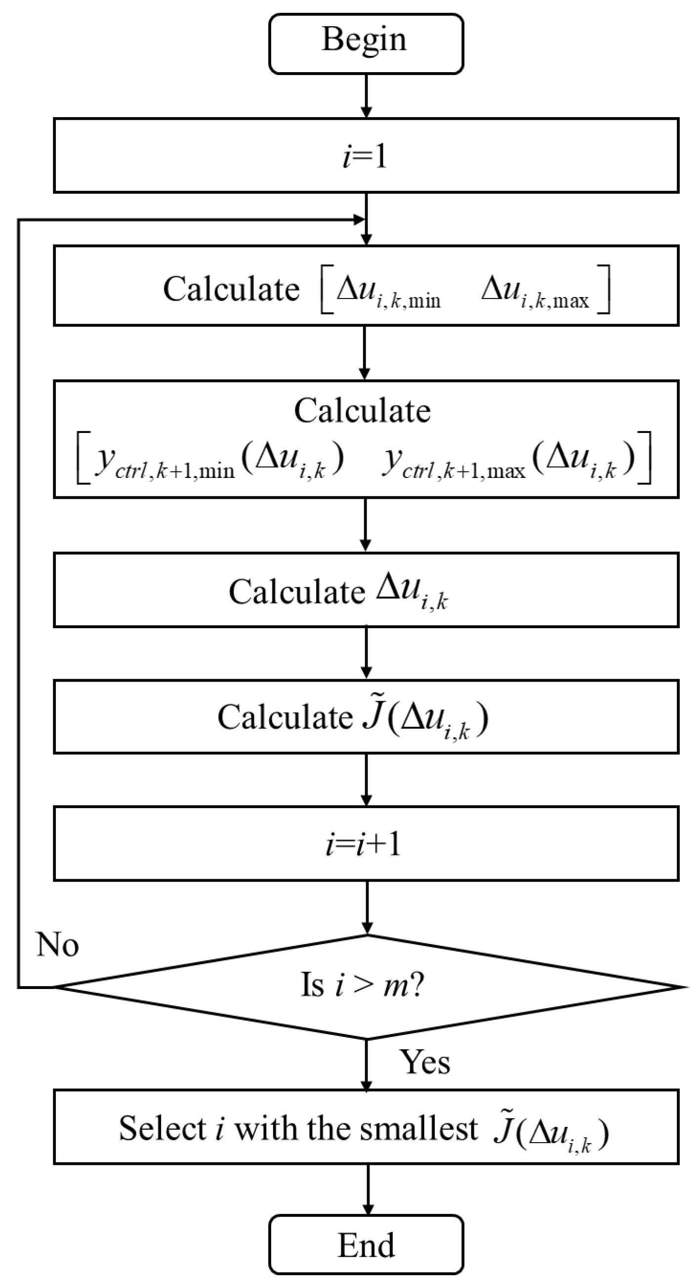
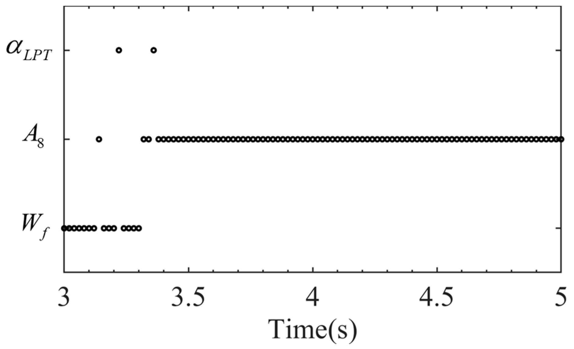
2.2. Control Variable Selection Algorithm
In fact, the control effect on the engine during the regulating process is accumulated by the control effect at each sampling instant, and the control effect at each sampling instant depends on the regulating ability of the selected control variable. Therefore, it is extremely necessary to consider which control variable is to be chosen at each sampling instant for better control results. However, the existing method, such as mMPC, does not pay enough attention to this selection issue. It changes the control variable sequentially and cyclically as the sampling instant increases, as shown in Figure 1. Essentially, it is an inflexible and non-intelligent selection mode. Since the regulating ability of each control variable is evidently not equivalent, an intelligent mode is needed to choose the suitable control variable at each sampling instant.
To achieve the intelligent mode, a control variable selection algorithm is designed to select the control variable that has the best control effect at the current sampling instant. According to the system information of the current sampling instant and the control target, the control effect of each control variable can be predicted for selection. The control variable selection algorithm is conducted as follows.
Firstly, the value range of each control variable at the first predicting instant is calculated. For example, at sampling instant k, the ith control variable at predicting instant k (i.e., ) should be able to meet the requirements of the constraints, that is, the limits of the control variable increment rate, the limits of the control variable increment magnitude and the limits of the constrained parameters’ increment.
According to Equations (13) and (14), the value range of can be calculated as
Then, the value range of the controlled parameters at predicting instant k + 1 can be computed as
By comparing with , the possible value of can be obtained.
In Equation (17), the first formula represents the value of that corresponds to and so does the third formula.
Subsequently, a merit function that considers the minimum control error and the possible control energy consumption is used to evaluate the control effect of .
In Equation (18), takes the corresponding value in Equation (17). The second formula indicates the case in which the control objective is in the range of the control variable’s regulating ability.
Finally, the merit functions of m control variables are calculated separately, and the control variable with the smallest merit function value is taken as the selected one.
The flowchart of the control variable selection algorithm at the current sampling instant can be illustrated as in Figure 2.
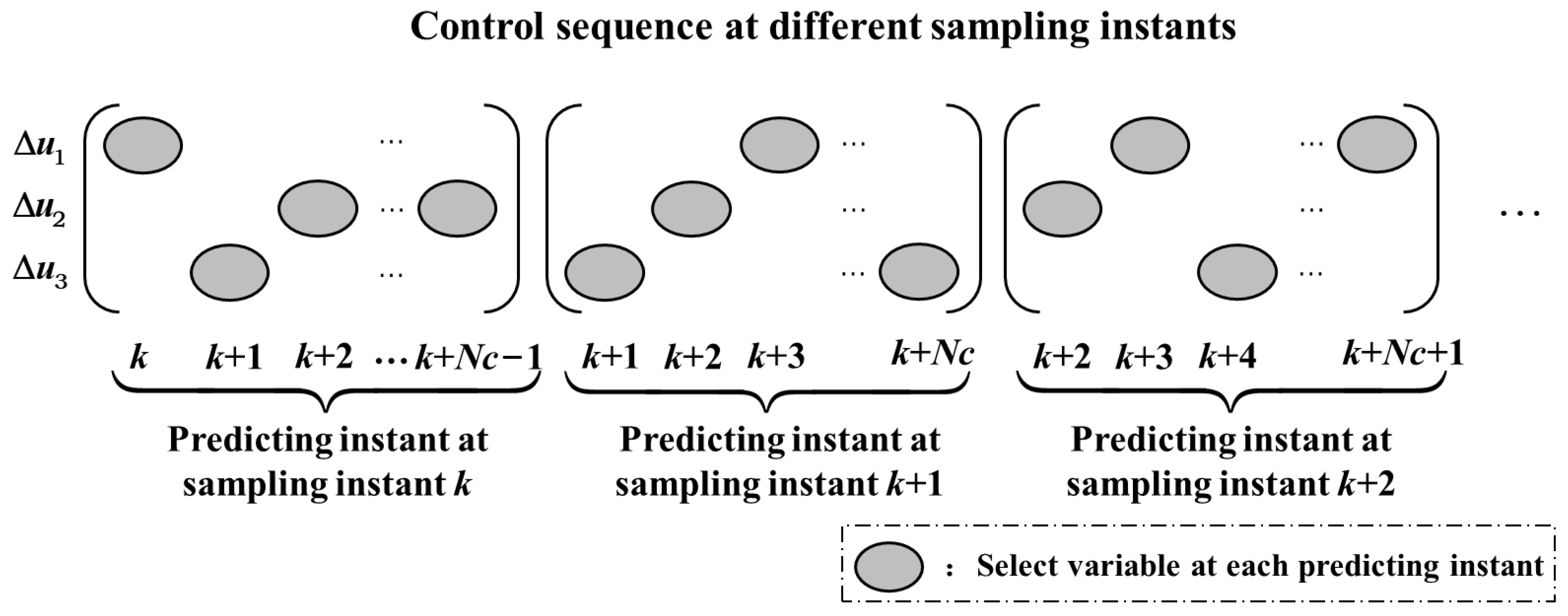
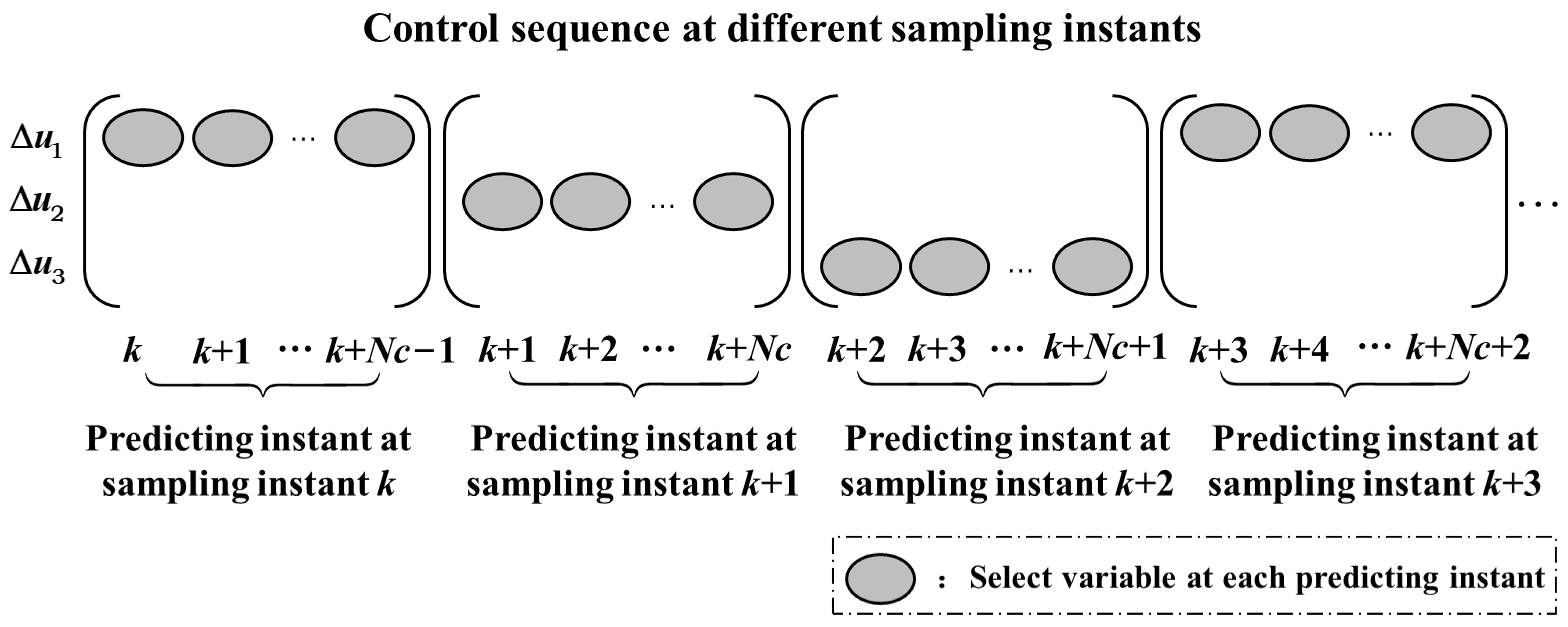
2.3. Control Sequence Coordination Strategy
Despite only the first element in the control sequence being fed to the engine, MPC actually predicts all the other elements, i.e., , by solving the constructed optimization problem. In the solution process, the result of each element will affect the others. For example, if the second element is another variable , the solution result of changes accordingly. Among the elements, each one represents the predictive value of the control variable at the corresponding sampling instant. According to Section 2.2, each sampling instant can select the best variable to be the control action. Assume that the variable at sampling instant k + 1 is ; it is better to employ as the second element in the control sequence of sampling instant k. This is true for the other sampling instants (k + 2, …, k + Nc − 1). Under this arrangement, can obtain a better solution to enhance the control performance since each element is selected properly, whereas all the elements are the same in mMPC, which neglects the interaction among the predicting instants in the control sequence.
The arrangement is called a control sequence coordination strategy. The strategy is conducted as follows to optimally select the variables at subsequent predicting instants in the control sequence.
Based on Section 2.2, the first element and its potential value in the control sequence can be determined as . Assuming that the second element is , it should also satisfy the constraints of control variable and constrained parameters.
In Equation (20), can be obtained with the help of Equations (2) and (3).
Similarly, the value range of and the value range of the controlled parameters at predicting instant k + 2 can be derived as
Then, the possible value of is
In the same way, to evaluate the control effect of , the merit function can be constructed as
By computing the m merit functions, the second element and its potential value in the control sequence can be determined. Then, accordingly, the variable that yields the optimal control effect at each predicting instant can be selected to form a coordinated control sequence, as illustrated in Figure 3.
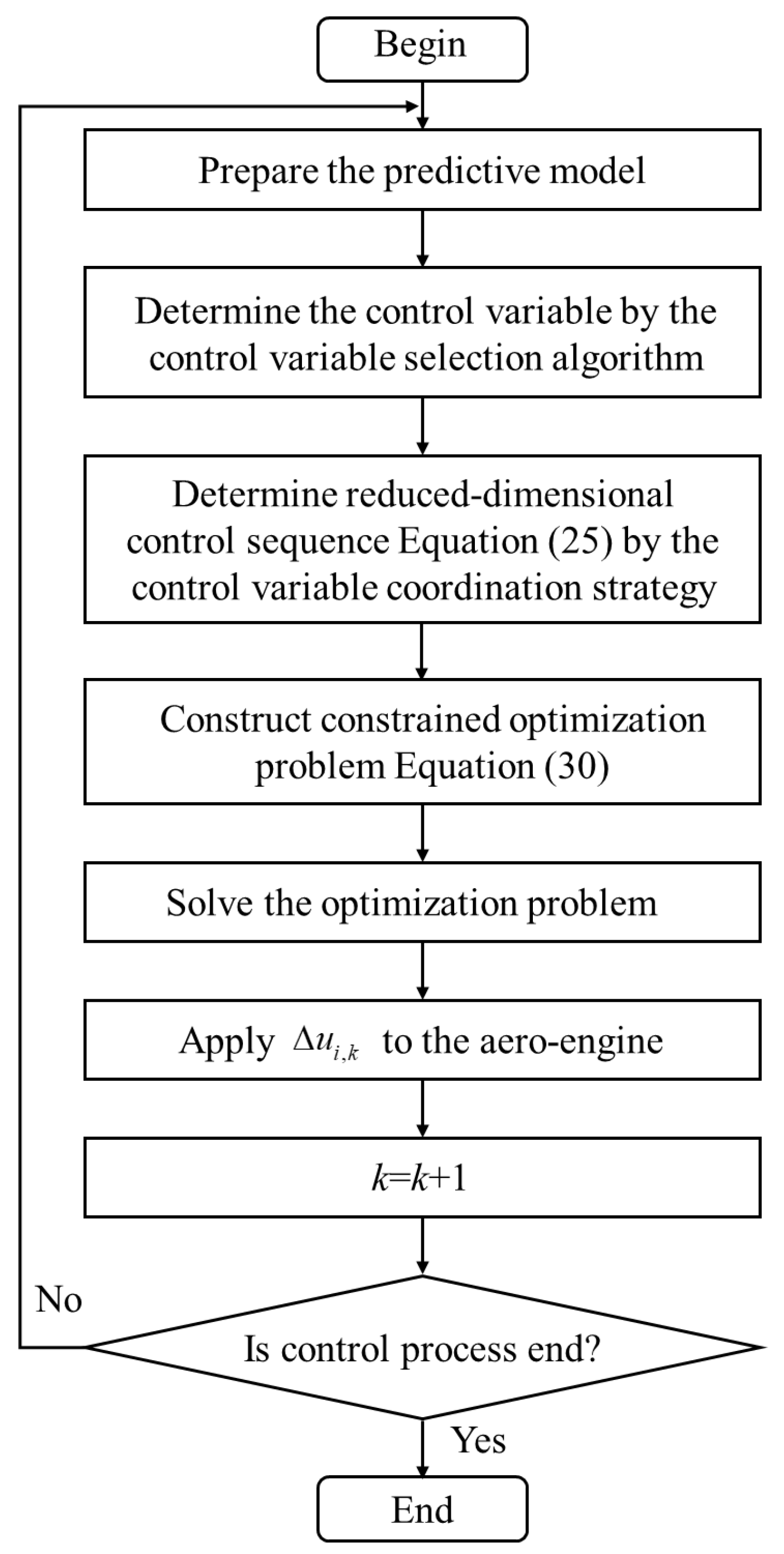
2.4. Intelligent Reduced-Dimensional MPC
Denote the coordinated control sequence as
where i, j and l separately represent the selected control variable at their corresponding predicting instants.
Based on Equation (25), a new constrained optimization problem can be constructed as follows. Firstly, Equation (5) can be rewritten as
where has a difference from in that the transfer matrix in each column should be changed according to Equation (25). The same is true for the matrix .
The cost function is also changed as
where .
Then, for the constrained parameters and control variables, the corresponding equations about limitation are
where
is a lower triangular matrix with diagonal elements all equal to 1. Except for the diagonal, for any two variables in the control sequence , .
Finally, the constrained optimization problem in the intelligent reduced-dimensional MPC can be abstracted as
where .
In summary, the proposed intelligent reduced-dimensional scheme has three key points. Firstly, reduce the dimension of control variables from m to 1 to lower the computational complexity of the optimization problem in MPC; secondly, determine the control variable with the best control effect at the current sampling instant by the control variable selection algorithm; finally, define a coordinated reduced-dimensional control sequence as Equation (25) with the help of the control variable coordination strategy and thus construct the constrained optimization problem Equation (30). By solving the optimization problem and applying the solution to the aero-engine, a receding horizon control process can operate. The flowchart of the proposed method is shown in Figure 4.
3. Simulation and Discussion
3.1. Simulation Cases
A twin-shaft turbofan engine with core driven fan stage (CDFS) is selected as the controlled object. The engine has components of intake, fan, CDFS, high-pressure compressor (HPC), combustor, high-pressure turbine (HPT), low-pressure turbine (LPT), duct and nozzle. By referring to the modeling method in [34,35] and using the Simulink Toolbox for the Modeling and Analysis of Thermodynamics Systems (T-MATS), the component-level model of this engine is constructed. In the model, all the co-operation equations are formulated based on aero-thermodynamics principles, flow continuity equations, pressure balance equations and rotor dynamics equations and are solved with the help of the Newton-Raphson method. All the components’ maps and performance data are acquired from GasTurb [36].
The input of the component-level model includes the flight condition [H, Ma] and the following control variables: the fuel flow , the nozzle area and the variable guide vane angle of LPT , i.e., . The output parameters are composed of the low-pressure rotor speed , the high-pressure rotor speed , the HPC exhaust pressure and the LPT exhaust temperature . Among them, is selected as the controlled parameter due to the strong correlation with thrust, while , and are considered the constrained parameters for safety operation, i.e., and .
To demonstrate the effectiveness of the proposed intelligent reduced-dimensional scheme, simulations are conducted at two flight conditions: [H, Ma] = [0, 0] and [H, Ma] = [11,000 m, 1.2]. In these conditions, the configuration of the engine is listed in Table 1 and Table 2, wherein = 20 ms is the sampling period.
A set value of = 2% is given as the control objective of both cases. A method is adopted to determine the reference trajectory based on the set value and the current value of the controlled parameter [37], wherein is a softening factor.
For each case, an intelligent reduced-dimensional linear MPC controller, denoted as “irdMPC” and shown in Figure 5, can be designed according to Section 2 and implemented to achieve the control targets. Concurrently, both the standard MPC controller and the multiplex MPC controller, denoted as “sMPC” and “mMPC”, respectively, are designed for comparative analysis.
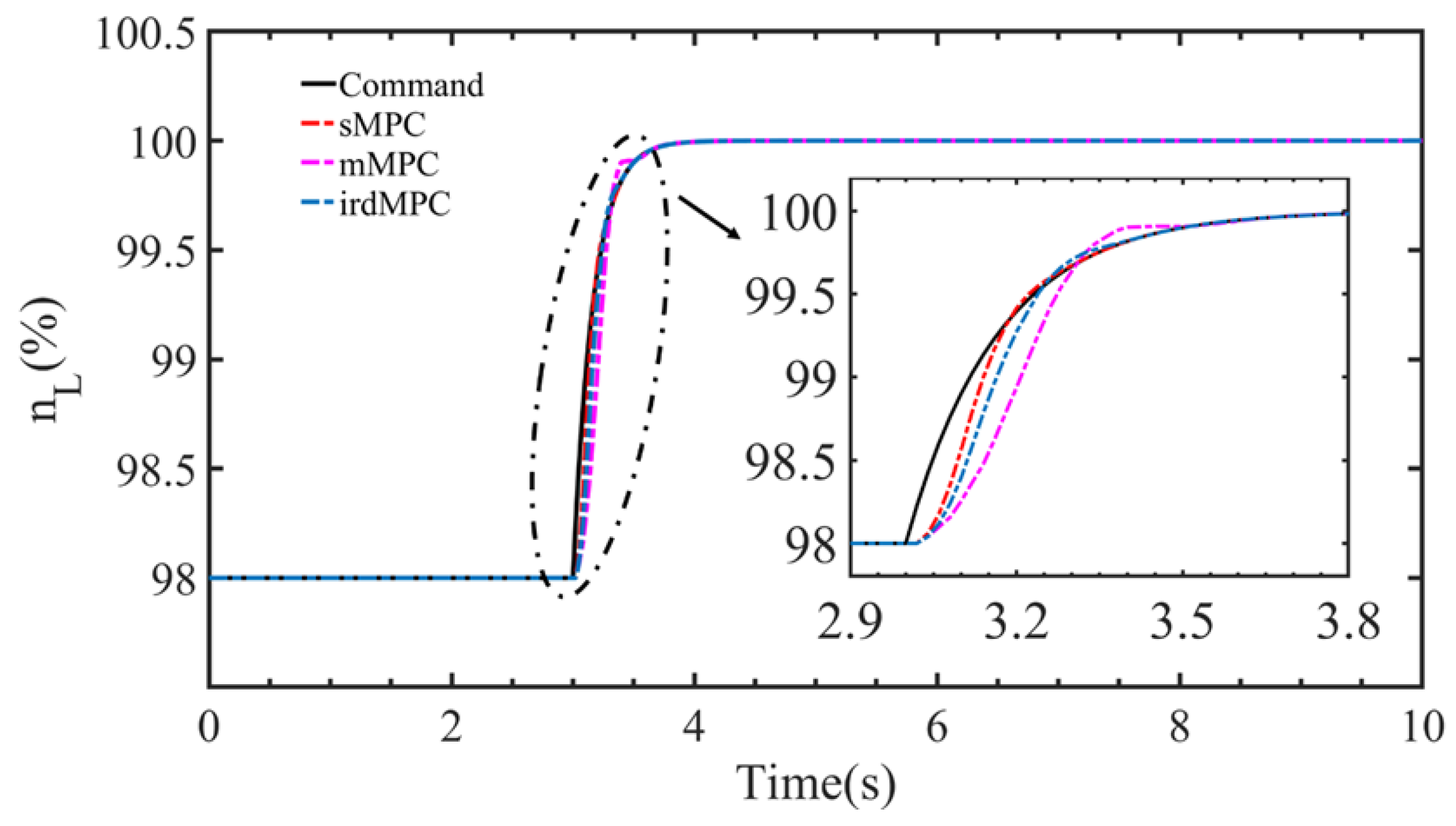
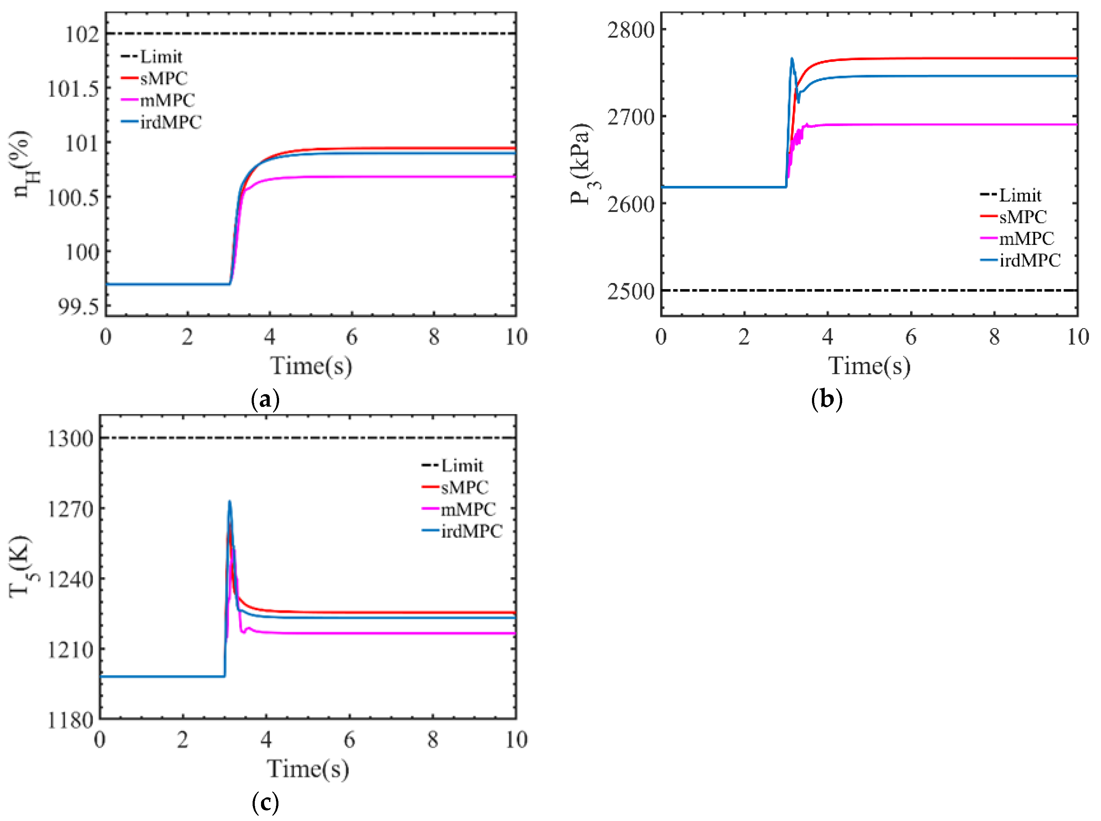
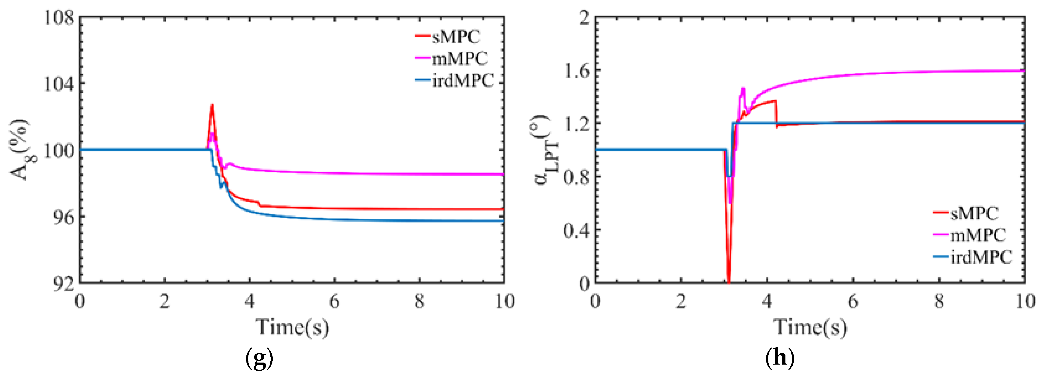
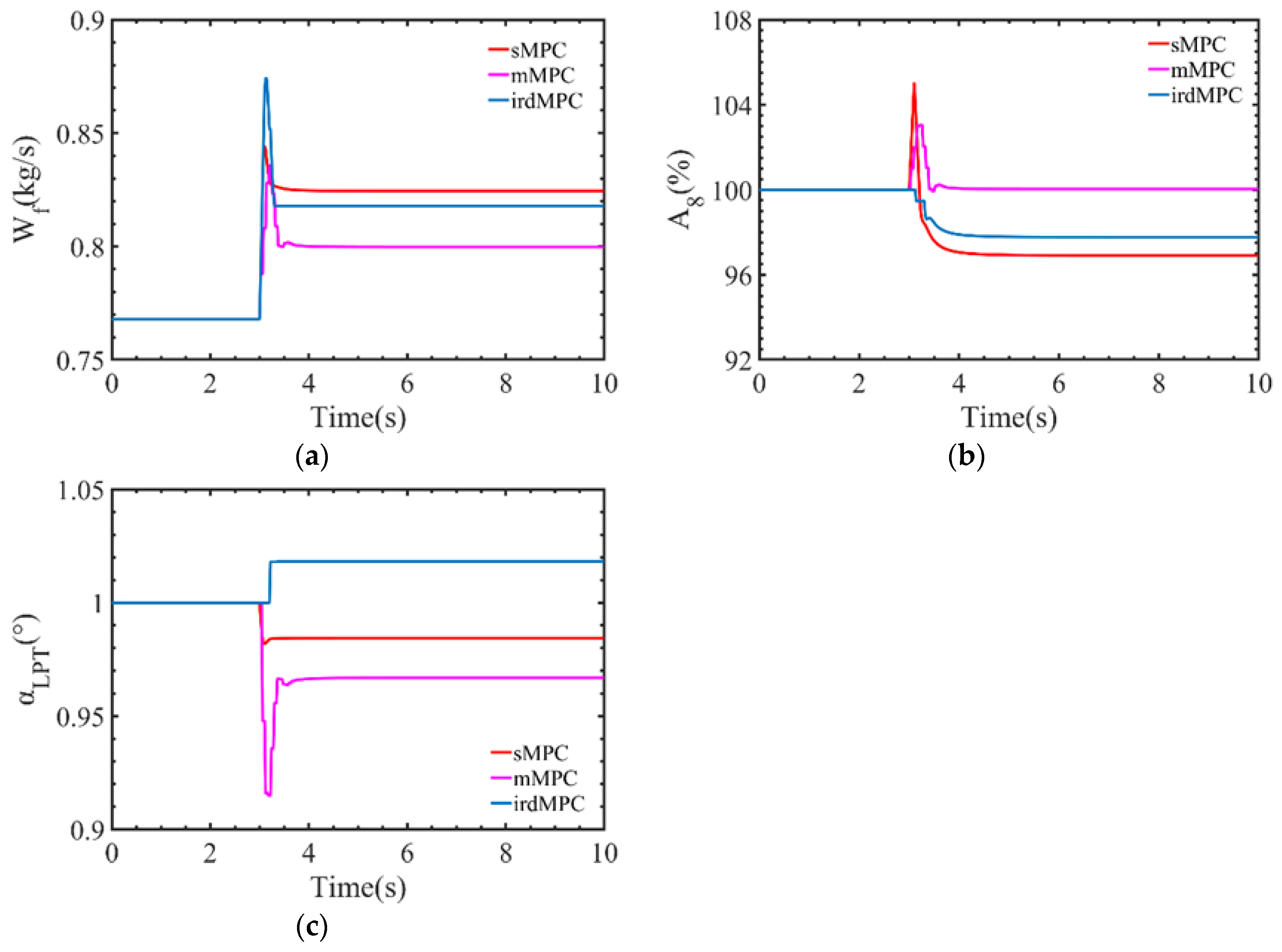
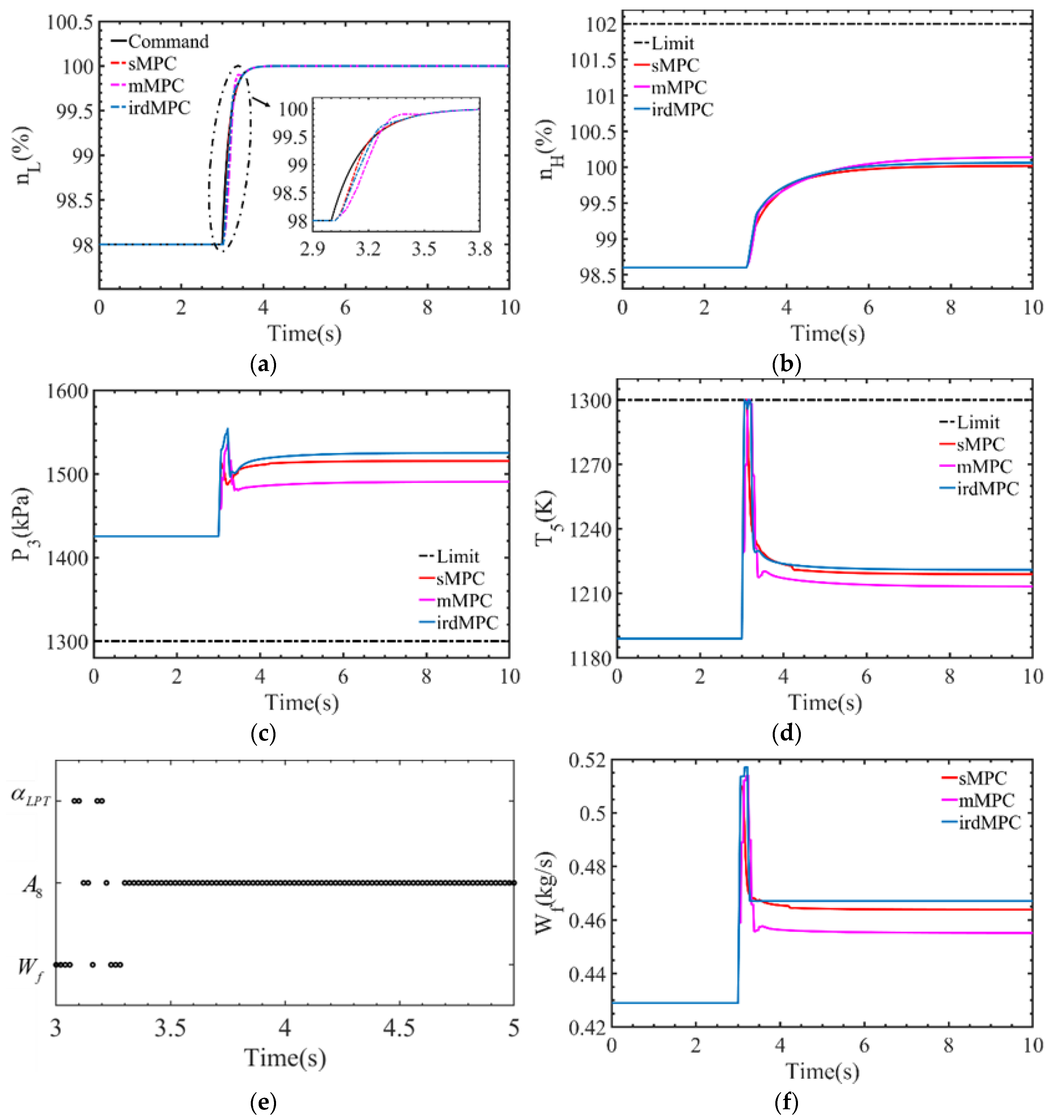
3.2. Control Effect Comparison
Firstly, a simulation is conducted at the flight condition [H, Ma] = [0, 0] to illustrate the effectiveness of the proposed method in control performance. During the simulation, the designed MPC controllers, which are “irdMPC”, “sMPC” and “mMPC”, adopt the same parameter settings, i.e., prediction horizon Np, control horizon Nc, weight matrices Q and R, in order to intuitively reflect the differences in control quality. By trial-and-error simulations, they can be well tuned. The controlled parameter’s response under the three MPC controllers is depicted in Figure 6. The constrained parameters are depicted in Figure 7.
Although all the MPC controllers can accomplish effective command tracking and constrains management, they actually have different performances. From Figure 6, it can be seen that “mMPC” witnesses a noticeable overshoot and long tracking response time. Thus, it has a poorer control outcome in command tracking than the others. “irdMPC” outperforms “mMPC”, but it is still slightly inferior to “sMPC”. The reason is that “irdMPC” and “mMPC” degrade their regulating ability by reducing the dimension of the control sequence. Nevertheless, “irdMPC” can track the reference trajectories well and has smaller tracking errors than “mMPC”, demonstrating the effectiveness of the intelligent reduced-dimensional scheme in achieving good control quality. In terms of constraint management, the constrain parameters of the three MPC controllers reach different values after the transition process, as shown in Figure 7. Similarly, “irdMPC” is closer to “sMPC” than “mMPC”, which represents that “irdMPC” derives a better operating state than “mMPC”. Moreover, “mMPC” has a certain oscillation during transition in Figure 7b.
The parameters’ response originates from the control variables’ changes. During the process, the control variables’ changes are shown in Figure 8. During transition, the selected control variable in “irdMPC” at each sampling instant is represented as “o” and is displayed in Figure 9.
In Figure 8, the control variables have various changes in the MPC controllers. Unlike “sMPC”, only one control variable is optimized in “mMPC” and “irdMPC” at each sampling instant. Moreover, the control variable to be optimized among them is also different. Thus, the results of solving constraints’ optimization problems, namely the changes of control variables, are different, resulting in their corresponding control outcomes. From Figure 9, it can be seen that the intelligent reduced-dimensional scheme selects for adjustment in the initial stage of transition, while it selects the three variables separately in the middle stage and in the final stage. This intelligent update mode makes the variables of “irdMPC” nearer to those of “sMPC” and thus leads to a better parameter response than “mMPC”. Although the change is different from the others, it has only a small impact on the overall results since the regulating ability of is the lowest among the variables.
For further comparison, the Root Mean Squared Error (RMSE) of the controlled parameter is calculated by Equation (32) to quantify the control errors of the controllers. Table 3 shows the RMSE of the three MPC controllers.
where N is the number of sample points.
By comparing the controllers’ RMSE, it can be seen that the multiplex MPC controller has much larger RMSE compared with the standard one. The RMSE of the “mMPC” is 2.11 times and differs by from that of “sMPC”. While “irdMPC” greatly decreases the control errors, it has an RMSE of and a 34.06% improvement in control performance over “mMPC”. Compared with “mMPC”, “irdMPC” significantly reduces the RMSE deviation from to , which indicates the superiority of the proposed intelligent reduced-dimensional scheme to the existing method, i.e., the multiplex MPC, in control performance.
3.3. Time Consumption Comparison
To illustrate the effectiveness of the proposed method in real-time performance, some simulations of different control horizons are conducted at the flight condition [H, Ma] = [0, 0]. During the simulation, the time required for the optimization solving processes in “irdMPC”, “sMPC” and “mMPC” are recorded and compared. Since the MPC controllers adopt the same configuration and the simulations implement the same test environment, the results make sense. Table 4 lists the average time of the optimization problem solving, which is defined as Equation (33) and denoted as “”.
In Table 4, the prediction horizon Np is equal to 10. It can be seen that the average time consumption of these MPC controllers increases as the control horizon increases. The increase in the control horizon leads to an increase in the dimension of the control sequence. Therefore, the computational complexity increases, resulting in the time required for the optimization solutions increasing, while under the same control horizon, “irdMPC” has a lower dimension of the control sequence compared with “sMPC” and thus has lower computational complexity and a shorter average time consumption. The average time consumption of “irdMPC” is 4.9351 ms when the control horizon is 3, while that of the “sMPC” is 6.3461 ms. The of “sMPC” is 1.286 times that of “irdMPC”. When the control horizon is 9, the of “irdMPC” is 6.148 ms, while that of “sMPC” is 17.4286 ms. The of “sMPC” becomes 2.835 times that of “irdMPC”. As the dimension of the control sequence increases, “irdMPC” reduces the of “sMPC” at most by 64.72%. Compared with “mMPC”, “irdMPC” has a slightly bigger time consumption as a result of the control variable selection algorithm and control sequence coordinate strategy embedded in the scheme bringing extra computational tasks. For the of “irdMPC” and “mMPC”, the ratio fluctuates between 1.016 and 1.1, which is small and acceptable considering a significant improvement in control performance. Furthermore, this ratio does not have a growing trend as the control horizon increases.
In the case of Nc = 5, some single-step time consumption results are listed in Table 5 to show details about the real-time performance comparison.
Table 5 records the time consumption of solving optimization problems at nine sampling instants. It can be seen that the results of these sampling instants are close to the values in Table 4. For each sampling instant, “sMPC” has larger solving time than “mMPC” and “irdMPC”. Owing to extra computational tasks, the time consumption of “irdMPC” is slightly bigger than that of “mMPC” at most of the sampling instants. Nevertheless, their results have a similar level, and there exist two sampling instants at which “irdMPC” has smaller results.
The above results and analysis demonstrate the superiority of the intelligent reduced-dimensional MPC controller in time consumption over the standard MPC controller. In a fixed sampling period during the control process, the intelligent reduced-dimensional MPC controller has the potential to operate under a bigger control horizon.
3.4. Further Verification
Under another flight condition [H, Ma] = [11,000 m, 1.2], simulations are implemented to further illustrate the effectiveness of the proposed method. Similar results can be seen in Figure 10 and Table 6.
Through the results under two flight conditions, the ability of the proposed intelligent reduced-dimensional scheme in achieving both good control performance and real-time performance is demonstrated, and the prospect of the designed intelligent reduced-dimensional MPC controller in regulating the aero-engine is validated.
4. Conclusions
For good control performance and real-time performance simultaneously, an intelligent reduced-dimensional scheme of model predictive control is proposed in this paper. By reducing the dimension of the control vector in the control sequence to 1, a reduced-dimensional optimization problem with low computational complexity is constructed. In the proposed scheme, a novel selection algorithm is proposed to intelligently select the control variable with the best control effect as the available one in the optimization problem. In addition, the scheme embeds a coordination strategy to take into account the interaction among the control variables at different predicting instants in order to obtain a better optimization solution.
Simulation examples are implemented to illustrate the effectiveness of the proposed method. The results are as follows: (1) by applying the intelligent reduced-dimensional scheme, the control error of the multiplex MPC is greatly improved by 34.06%; (2) the intelligent reduced-dimensional scheme guarantees superiority in computational complexity. Compared to the standard MPC, it can save average time consumption by up to 64.72% when the control horizon increases to nine. All the results demonstrate that the proposed method has not only a better control outcome than the multiplex MPC but also less computation time than the standard MPC and thus helps the implementation of the MPC controller in the aero-engine.
The limitation of the proposed intelligent reduced-dimensional scheme is that this methodology is currently suitable for linear MPC, so the extension to nonlinear MPC needs further research. In addition, only numerical simulations are conducted in this paper to illustrate the effectiveness of the method. For further verification, the hardware-in-the-loop experiment will be considered in future research.
Author Contributions
Conceptualization, Z.J. and X.W.; methodology, Z.J. and J.L.; software, Z.J. and N.G.; validation, Z.J. and W.L; formal analysis, N.G.; investigation, W.L.; resources, X.W.; data curation, Z.J. and J.L.; writing—original draft preparation, Z.J.; writing—review and editing, X.W., N.G. and W.L.; visualization, Z.J.; supervision, X.W.; project administration, X.W. All authors have read and agreed to the published version of the manuscript.
Funding
This research received no external funding.
Data Availability Statement
The data that support the findings of this study are available from the corresponding author upon reasonable request.
Conflicts of Interest
Author Wei Liu was employed by the company China Gas Turbine Establishment. The remaining authors declare that the research was conducted in the absence of any commercial or financial relationships that could be construed as a potential conflict of interest.
References
Wang, X.; Yang, S.; Zhu, M.; Kong, X.X. Aeroengine Control Principles; Science Press: Beijing, China, 2021. [Google Scholar]
Garg, S. Introduction to Advanced Engine Control Concepts; NASA Glenn Research Center: Cleveland, OH, USA, 2007.
Zhu, Y.; Pan, M.; Zhou, W.; Huang, J. Intelligent direct thrust control for multivariable turbofan engine based on reinforcement and deep learning methods. Aerosp. Sci. Technol.2022, 131, 107972. [Google Scholar] [CrossRef]
Akpan, V.A.; Hassapis, G.D. Nonlinear model identification and adaptive model predictive control using neural networks. ISA Trans.2011, 50, 177–194. [Google Scholar] [CrossRef] [PubMed]
Bing, Y.U.; Zhouyang, L.I.; Hongwei, K.E.; Zhang, T. Wide-range model predictive control for aero-engine transient state. Chin. J. Aeronaut.2022, 35, 246–260. [Google Scholar]
Chen, Q.; Sheng, H.; Zhang, T. A novel direct performance adaptive control of aero-engine using subspace-based improved model predictive control. Aerosp. Sci. Technol.2022, 128, 107760. [Google Scholar] [CrossRef]
Richalet, J.; Rault, A.; Testud, J.L.; Papon, J. Model predictive heuristic control. Automatica1978, 14, 413–428. [Google Scholar] [CrossRef]
Cutler, C.R.; Ramaker, B.L. Dynamic matrix control—A computer control algorithm. In Proceedings of the Joint Automatic Control Conference, San Francisco, CA, USA, 13–15 August 1980; p. 72. [Google Scholar]
Liu, J.; Wang, X.; Liu, X.; Zhu, M.; Pei, X.; Zhang, S.; Dan, Z. μ-Synthesis control with reference model for aeropropulsion system test facility under dynamic coupling and uncertainty. Chin. J. Aeronaut.2023, 36, 246–261. [Google Scholar] [CrossRef]
Liu, J.; Wang, X.; Liu, X.; Zhu, M.; Pei, X.; Dan, Z.; Zhang, S. μ-Synthesis-based robust L1 adaptive control for aeropropulsion system test facility. Aerosp. Sci. Technol.2023, 140, 108457. [Google Scholar] [CrossRef]
Liu, J.; Wang, X.; Liu, X.; Pei, X.; Dan, Z.; Zhang, S.; Yang, S.; Zhang, L. An anti-windup design with local sector and H2/H∞ optimization for flight environment simulation system. Aerosp. Sci. Technol.2022, 128, 107787. [Google Scholar] [CrossRef]
Richter, H. Advanced Control of Turbofan Engines; Springer Science & Business Media: Berlin/Heidelberg, Germany, 2011. [Google Scholar]
Brunell, B.J.; Viassolo, D.E.; Prasanth, R. Model adaptation and nonlinear model predictive control of an aircraft engine. In Proceedings of the Turbo Expo: Power for Land, Sea, and Air, Vienna, Austria, 14–17 June 2004; pp. 673–682. [Google Scholar]
Wang, Y.; Huang, J.; Zhou, W.; Lu, F.; Hu, W. Neural network-based model predictive control with fuzzy-SQP optimization for direct thrust control of turbofan engine. Chin. J. Aeronaut.2022, 35, 59–71. [Google Scholar] [CrossRef]
Wang, Y.; Zheng, Q.G.; Du, Z.Y.; Zhang, H. Research on nonlinear model predictive control for turboshaft engines based on double engines torques matching. Chin. J. Aeronaut.2020, 33, 176–186. [Google Scholar] [CrossRef]
Nikolaidis, T.; Li, Z.; Jafari, S. Advanced constraints management strategy for real-time optimization of gas turbine engine transient performance. Appl. Sci.2019, 9, 5333. [Google Scholar] [CrossRef]
Boyd, S.P.; Vandenberghe, L. Convex Optimization; Cambridge University Press: Cambridge, UK, 2004. [Google Scholar]
Kochenderfer, M.J.; Wheeler, T.A. Algorithms for Optimization; MIT Press: Cambridge, MA, USA, 2019. [Google Scholar]
Bemporad, A.; Morari, M.; Dua, V.; Pistikopoulos, E.N. The explicit solution of model predictive control via multiparametric quadratic programming. In Proceedings of the 2000 American Control Conference, ACC (IEEE Cat. No. 00CH36334), Chicago, IL, USA, 28–30 June 2000; IEEE: Piscataway, NJ, USA, 2000; Volume 2, pp. 872–876. [Google Scholar]
Tøndel, P.; Johansen, T.A.; Bemporad, A. An algorithm for multi-parametric quadratic programming and explicit MPC solutions. Automatica2003, 39, 489–497. [Google Scholar] [CrossRef]
Alessio, A.; Bemporad, A. A survey on explicit model predictive control. In Nonlinear Model Predictive Control: Towards New Challenging Applications; Springer: Berlin/Heidelberg, Germany, 2009; pp. 345–369. [Google Scholar]
Gu, N.; Wang, X.; Zhu, M. Multi-Parameter Quadratic Programming Explicit Model Predictive Based Real Time Turboshaft Engine Control. Energies2021, 14, 5539. [Google Scholar] [CrossRef]
Feng, C.; Du, X.; Yang, B. Design of Turbofan Engine Controller Based on Explicit Predictive Control. J. Propuls. Technol.2022, 6, 043. [Google Scholar]
Lewis, F.L.; Vrabie, D.; Syrmos, V.L. Optimal Control; John Wiley & Sons: Hoboken, NJ, USA, 2012. [Google Scholar]
Genceli, H.; Nikolaou, M. Robust stability analysis of constrained l1-norm model predictive control. AIChE J.1993, 39, 1954–1965. [Google Scholar] [CrossRef]
Kerrigan, E.C.; Maciejowski, J.M. Robustly stable feedback min-max model predictive control. In Proceedings of the 2003 American Control Conference, Denver, CO, USA, 4–6 June 2003; IEEE: Piscataway, NJ, USA, 2003; Volume 4, pp. 3490–3495. [Google Scholar]
Wang, X.Q.; Ho, W.K.; Ling, K.V. Computational load comparison of multiplexed and standard model predictive control. In Proceedings of the 2018 4th International Conference on Mechatronics and Robotics Engineering, Valenciennes, France, 7–11 February 2018; pp. 17–22. [Google Scholar]
Ling, K.V.; Maciejowski, J.; Wu, B.F. Multiplexed model predictive control. IFAC Proc. Vol.2005, 38, 574–579. [Google Scholar] [CrossRef]
Ling, K.V.; Ho, W.K.; Wu, B.F.; Lo, A.; Yan, H. Multiplexed MPC for multizone thermal processing in semiconductor manufacturing. IEEE Trans. Control Syst. Technol.2009, 18, 1371–1380. [Google Scholar] [CrossRef]
Richter, H.; Singaraju, A.V.; Litt, J.S. Multiplexed predictive control of a large commercial turbofan engine. J. Guid. Control Dyn.2008, 31, 273–281. [Google Scholar] [CrossRef]
Pang, S.; Jafari, S.; Nikolaidis, T.; Qiuhong, L.I. Reduced-dimensional MPC controller for direct thrust control. Chin. J. Aeronaut.2022, 35, 66–81. [Google Scholar] [CrossRef]
Pang, S.; Li, Q.; Ni, B. Improved nonlinear MPC for aircraft gas turbine engine based on semi-alternative optimization strategy. Aerosp. Sci. Technol.2021, 118, 106983. [Google Scholar] [CrossRef]
Liu, Z.W.; Wang, Z.X.; Huang, H.C.; Cai, J.H. Numerical simulation on performance of variable cycle engines. J. Aero-Space Power2010, 25, 1310–1315. [Google Scholar]
Wang, Y.; Zhang, P.P.; Li, Q.H.; Huang, X.H. Research and validation of variable cycle engine modeling method. J. Aerosp. Power2014, 29, 2643–2651. [Google Scholar]
Kurzke, J. GasTurb 12: Design and Off-Design Performance of Gas Turbines; Mtu: Munich, Germany, 2012. [Google Scholar]
Du, X. Application of Sliding Mode Control and Model Predictive Control to Limit Management for Aero-Engines; Northwestern Polytechnical University: Xi’an, China, 2016. [Google Scholar]
Figure 1.
Schematic of the update mode of 3 control variables in mMPC.
Figure 1.
Schematic of the update mode of 3 control variables in mMPC.
Figure 2.
Flowchart of the control variable selection algorithm.
Figure 2.
Flowchart of the control variable selection algorithm.
Figure 3.
Schematic of the update mode of 3 control variables in the proposed scheme.
Figure 3.
Schematic of the update mode of 3 control variables in the proposed scheme.
Figure 4.
Flowchart of the intelligent reduced-dimensional MPC.
Figure 4.
Flowchart of the intelligent reduced-dimensional MPC.
Figure 5.
Control structure of “irdMPC” in Simulink environment.
Figure 5.
Control structure of “irdMPC” in Simulink environment.
Figure 6.
Controlled parameters’ response under “sMPC”, “mMPC” and “irdMPC”.
Figure 6.
Controlled parameters’ response under “sMPC”, “mMPC” and “irdMPC”.
Figure 7.
Constrained parameters’ response under “sMPC”, “mMPC” and “irdMPC”. (a) response curve. (b) response curve. (c) response curve.
Figure 7.
Constrained parameters’ response under “sMPC”, “mMPC” and “irdMPC”. (a) response curve. (b) response curve. (c) response curve.
Figure 8.
Control variables’ changes under “sMPC”, “mMPC” and “irdMPC”. (a) change curve. (b) change curve. (c) change curve.
Figure 8.
Control variables’ changes under “sMPC”, “mMPC” and “irdMPC”. (a) change curve. (b) change curve. (c) change curve.
Figure 9.
Selected control variable at each sampling instant during transition in “irdMPC”.
Figure 9.
Selected control variable at each sampling instant during transition in “irdMPC”.
Figure 10.
Simulation results for control performance at [H, Ma] = [11,000 m, 1.2]. (a) response curve. (b) response curve. (c) response curve. (d) response curve. (e) Selected control variable at each sampling instant during transition in “irdMPC”. (f) change curve. (g) change curve. (h) change curve.
Table 1.
The configuration of the engine at [H, Ma] = [0, 0].
Table 1.
The configuration of the engine at [H, Ma] = [0, 0].
Parameters
Initial Steady-State Value
Magnitude Limit
Rate Limit
Unit
Output
98
%
99.7
%
2618.4
kPa
1198.2
K
Control variable
0.768
0.03/
kg/s
100
0.5/
%
1
0.2/
°
Table 2.
The configuration of the engine at [H, Ma] = [11,000 m, 1.2].
Table 2.
The configuration of the engine at [H, Ma] = [11,000 m, 1.2].
Parameters
Initial Steady-State Value
Magnitude Limit
Rate Limit
Unit
Output
98
%
98.6
%
1425.4
kPa
1189
K
Control variable
0.429
0.03/
kg/s
100
0.5/
%
1
0.2/
°
Table 3.
RMSE comparison of “sMPC”, “mMPC” and “irdMPC”.
Table 3.
RMSE comparison of “sMPC”, “mMPC” and “irdMPC”.
sMPC
mMPC
irdMPC
RMSE (×10−2)
3.8146
8.046
5.3057
Table 4.
Average time comparison of the “sMPC”, “mMPC” and “irdMPC”.
Table 4.
Average time comparison of the “sMPC”, “mMPC” and “irdMPC”.
Nc
(ms)
sMPC
mMPC
irdMPC
3
6.3461
4.858
4.9351
4
7.4579
4.9323
5.1989
5
9.1945
5.0723
5.4687
6
11.111
5.2522
5.6339
7
13.2113
5.3438
5.8783
8
15.2596
5.5492
6.008
9
17.4286
5.6789
6.148
Table 5.
Single-step time comparison of “sMPC”, “mMPC” and “irdMPC”.
Table 5.
Single-step time comparison of “sMPC”, “mMPC” and “irdMPC”.
Sampling Instant
t (ms)
sMPC
mMPC
irdMPC
k + 1
9.1861
5.2361
4.8048
k + 2
8.3069
5.3285
6.2879
k + 3
9.2412
4.9081
6.1662
k + 4
9.6713
4.9276
5.6472
k + 5
13.01
5.7536
4.8898
k + 6
10.3904
5.104
6.2612
k + 7
7.2827
5.2765
5.421
k + 8
7.7749
4.976
5.3001
k + 9
9.7422
4.8451
5.6359
Table 6.
Simulation results for real-time performance at [H, Ma] = [11,000 m, 1.2].
Table 6.
Simulation results for real-time performance at [H, Ma] = [11,000 m, 1.2].
Nc
(ms)
sMPC
mMPC
irdMPC
3
6.3336
5.0491
5.1505
4
8.0574
5.0809
5.3599
5
9.8516
5.1691
5.603
6
11.8859
5.4101
5.7942
7
14.5266
5.4756
5.9671
8
16.6374
5.6881
6.1405
9
19.3425
5.8344
6.2934
Disclaimer/Publisher’s Note: The statements, opinions and data contained in all publications are solely those of the individual author(s) and contributor(s) and not of MDPI and/or the editor(s). MDPI and/or the editor(s) disclaim responsibility for any injury to people or property resulting from any ideas, methods, instructions or products referred to in the content.
Jiang, Z.; Wang, X.; Liu, J.; Gu, N.; Liu, W.
Intelligent Reduced-Dimensional Scheme of Model Predictive Control for Aero-Engines. Actuators2024, 13, 140.
https://doi.org/10.3390/act13040140
AMA Style
Jiang Z, Wang X, Liu J, Gu N, Liu W.
Intelligent Reduced-Dimensional Scheme of Model Predictive Control for Aero-Engines. Actuators. 2024; 13(4):140.
https://doi.org/10.3390/act13040140
Chicago/Turabian Style
Jiang, Zhen, Xi Wang, Jiashuai Liu, Nannan Gu, and Wei Liu.
2024. "Intelligent Reduced-Dimensional Scheme of Model Predictive Control for Aero-Engines" Actuators 13, no. 4: 140.
https://doi.org/10.3390/act13040140
Note that from the first issue of 2016, this journal uses article numbers instead of page numbers. See further details here.
Article Metrics
No
No
Article Access Statistics
For more information on the journal statistics, click here.
Multiple requests from the same IP address are counted as one view.
Jiang, Z.; Wang, X.; Liu, J.; Gu, N.; Liu, W.
Intelligent Reduced-Dimensional Scheme of Model Predictive Control for Aero-Engines. Actuators2024, 13, 140.
https://doi.org/10.3390/act13040140
AMA Style
Jiang Z, Wang X, Liu J, Gu N, Liu W.
Intelligent Reduced-Dimensional Scheme of Model Predictive Control for Aero-Engines. Actuators. 2024; 13(4):140.
https://doi.org/10.3390/act13040140
Chicago/Turabian Style
Jiang, Zhen, Xi Wang, Jiashuai Liu, Nannan Gu, and Wei Liu.
2024. "Intelligent Reduced-Dimensional Scheme of Model Predictive Control for Aero-Engines" Actuators 13, no. 4: 140.
https://doi.org/10.3390/act13040140
Note that from the first issue of 2016, this journal uses article numbers instead of page numbers. See further details here.