Abstract
This study delves into the construction of reduced-order models (ROMs) of a flow field over a NACA 0012 airfoil at a moderate Reynolds number and an angle of attack of . Numerical simulations were computed through the finite-volume solver OpenFOAM. The analysis considers two different reduction techniques: the standard Galerkin projection method, which involves projecting the governing equations onto proper orthogonal decomposition modes (POD−ROMs), and the cluster-based network model (CNM), a fully data-driven nonlinear approach. An analysis of the topology of the dominant POD modes was conducted, uncovering a traveling wave pattern in the wake dynamics. We compared the performances of both ROM techniques regarding their prediction of flow field behavior and integral quantities. The ROM framework facilitates the practical actuation of control strategies with significantly reduced computational demands compared to the full-order approach.
1. Introduction
The quest to enhance aircraft performance, specifically in terms of drag reduction and improving the lift–drag ratio, is a paramount objective in aircraft design (Couto and Bergada [1] Chiatto et al. [2]). To achieve these goals, the incorporation of flow control mechanisms, such as synthetic jets (Ceglia et al. [3], Girfoglio et al. [4], de Luca et al. [5]), has proven beneficial for delaying separation and managing turbulence transition (Tousi et al. [6,7]). Through careful optimization of airfoil shapes and control parameters, lift, drag, and virtual mass can be tailored to meet specific flight envelope requirements (Lahey et al. [8]). However, this optimization process often necessitates many computational simulations, which can be both time-consuming and computationally intensive (Li et al. [9], Reumschüssel et al. [10], Wang et al. [11]).
Modal decomposition techniques have emerged as valuable tools for gaining a deeper understanding of the key coherent flow structures (Taira et al. [12]) and for designing effective control strategies (Rowley and Dawson [13]). The recent increase in computational capabilities has paved the way for the development of various data-driven analytical tools for different aspects of fluid dynamics, including spectral characterization (Schmid [14]), system frequency response (Herrmann et al. [15]), and even the study of two-phase flows (Schmidt and Oberleithner [16]).
Recent research, as highlighted by Stabile et al. [17], emphasizes the relevance of formulating reduced-order models (ROMs) that retain the key features of full-order models (FOMs) while significantly reducing computational demands. This step is crucial for simplifying the governing equations’ complexity and enhancing the efficiency of the optimization process (Noack et al. [18]).
As a matter of fact, when employing reduced-order models one encounters several drawbacks, for instance, the introduction of unphysical artifacts and instabilities (Noack et al. [19]), the loss of fidelity at fine temporal and spatial scales (Taira et al. [20]), and the inability to accurately predict rare or extreme events due to nonlinear interactions (Racca and Magri [21]). Cluster-based network modeling (CNM) stands as a robust approach for investigating complex nonlinear dynamics using data (Fernex et al. [22]). CNM relies on an unsupervised machine learning technique to process a dataset of snapshots, reducing them to a small set of representative flow states. Subsequently, statistical methods are employed to construct a reduced-order model that presents a probabilistic representation of the system dynamics. CNM offers a fully automated framework for understanding system dynamics (Hou et al. [23], Colanera et al. [24]), estimating parameters, and implementing model-based control (Wang et al. [25]).
Furthermore, recent advancements in machine learning techniques (Brunton et al. [26]) have demonstrated their effectiveness, even in the prediction of stall behavior (Saetta et al. [27]).
This study aims to develop reduced-order models (ROMs) for analyzing the flow around a specific airfoil configuration. Two distinct types of low-order models were constructed: proper orthogonal decomposition (POD) Galerkin ROMs (Stabile and Rozza [28]), which involve projecting the governing equations onto selected POD modes and cluster-based network models (CNMs) (Kaiser et al. [29] and Li et al. [30]). To the authors’ best knowledge, this paper represents an original application by comparing these two model approaches for airfoil configurations. This paper constitutes an expanded version of the conference paper by Di Costanzo et al. [31].
2. Methodology
This section provides an overview of full-order modeling for unsteady turbulent flow analysis. Additionally, it describes two different approaches to reduced-order modeling. Full-order modeling offers a detailed representation of the flow field but can be computationally expensive. Reduced-order modeling techniques offer a more efficient alternative by capturing essential flow features while reducing computational costs.
2.1. Full Order Model
The present study investigates the behavior of NACA0012 airfoil under two-dimensional, unsteady, and incompressible flow conditions. To tackle this problem, Unsteady Reynolds-averaged Navier–Stokes (URANS) equations were employed. The numerical simulations were conducted using the pimpleFoam solver within the open-source software OpenFOAM. The pimpleFoam employs the PIMPLE algorithm for pressure–velocity coupling, enabling the modeling of a transient flow within a discretized domain, achieved by solving the Reynolds-averaged Navier–Stokes equations.
For the representation of turbulence in this analysis, the well-established turbulence model was implemented. In this context, the equations system is denoted as a full-order model (FOM), as detailed in Equations (1) and (2).
where the time variable, t, kinematic pressure, p, and the velocity vector, , represented as , are considered. The effective kinematic viscosity is denoted as , where denotes the kinematic viscosity and denotes turbulent eddy viscosity. It is worth noting that in this work any additional effect related to the virtual mass has not been considered. The Reynolds number under free-stream conditions is defined as , where represents the free-stream velocity, and c is the airfoil chord. The angle of attack, denoted as , is fixed at for this investigation.
The simulations based on the FOM are executed until the values of time-averaged flow variables (such as velocity, drag, lift, and virtual mass when applicable) reach the periodic behavior. Subsequently, snapshots of flow field variables are stored for later use in constructing low-order models.
Utilizing the URANS approach and the turbulence model, the FOM describes the unsteady turbulent flow surrounding the NACA0012 airfoil. This forms the basis for subsequent analyses and the creation of reduced-order models.
2.2. POD–ROM
Adopting the methodology outlined in Hijazi et al. [32], one can employ a systematic process that combines the POD technique with Galerkin projections to derive reduced-order models (ROMs) from simulations or experimental data.
Specifically, one can express the truncation of the POD expansions for the discretized fields of velocity , pressure p, and eddy viscosity , as follows:
where , , and are, respectively, the POD mode matrices of velocity, pressure, and eddy viscosity. The computation of these mode matrices follows the procedure described by Stabile and Rozza [28], utilizing numerical data derived from the FOM.
The momentum equation is subsequently projected onto the modes represented by , resulting in the following reduced-order system:
Here, , , and denote the coefficients associated with the velocity, eddy viscosity, and pressure fields, respectively. Additional equations to determine coefficients and are derived from the pressure Poisson equation and the eddy viscosity model projections. Initial conditions for and are set by projecting and onto the POD modes. To stabilize the pressure, a velocity space supremizer enrichment strategy is employed, as detailed by Ballarin et al. [33]. The entire procedure is implemented using ITHACA-FV, a C++ library developed in the OpenFOAM framework [28].
The combination of proper orthogonal decomposition (POD) and Galerkin projections presents an effective method for constructing reduced-order models. This approach enables efficient analysis and prediction of flow patterns, substantially lowering computational costs.
2.3. CNM–ROM
The cluster-based network model (CNM) approach depicts the dynamics of a system through a directed network, wherein the clusters (i.e. the nodes) symbolize coarse-grained states of the system. The original snapshots are clustered into a few centroids representing the whole ensemble.
The clusters are computed using the standard k-means++ algorithm (MacQueen [34]; Lloyd [35]), which minimizes the inner-cluster variance. Consequently, the cost function J is defined as follows:
where M represents the number of snapshots used for the analysis, denotes the m-th snapshot of velocity components, and denotes the cluster to which belongs. The cluster-affiliation function associates a snapshot with the index of its nearest centroid:
where denotes a spatial norm. The optimal centroids, , are those that minimize J:
After the snapshots are coarse-grained into K clusters, each cluster can be seen as a representative state of the system dynamics. The network nodes are identified as centroids, , of these clusters, calculated as the state averages within each cluster. The transition characteristics between such clusters rely on high-order direct transition probabilities identified from the data [22].
As sketched in Figure 1, CNM utilizes the direct transition matrix Q, which considers only intercluster transitions and ignores the inner-cluster residence probability.
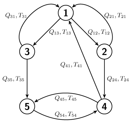
Figure 1.
Sketch of a directed network of clusters. The nodes denote cluster centroids, while arrows represent transition directions. Each transition includes a transition probability and time .
The direct transition probability is inferred from the data as follows:
where represents the probability of transitioning from cluster to , and denotes the number of such transitions, with being the total number of transitions departing from cluster j. Figure 1 shows an example of a directed network of clusters. For a generalized L-order model, the direct transition probability is expressed as (L being the model order), which is equivalent to using time-delay coordinates. Note that in the CNM framework, .
The residence time corresponds to the duration of the transit in a cluster , where and denote the time of the first and last snapshots to enter and leave . The individual transition time from cluster j to cluster k is defined as half the residence time of both clusters:
By averaging all individual transition times from cluster to , the transition time is estimated.
Once the probabilistic model is determined through matrices Q and T, a sequence of centroids, denoted as , can be determined together with with the following time instance:
In this framework, a smooth motion between these discrete jumps is obtained by a linear interpolation.
Within the CNM framework, the N-dimensional state of the system can be represented by various options, including the flow field variables themselves or any other observables. In this study, we consider the POD temporal coefficients as state vector components. Transition probabilities from one cluster centroid to another are estimated based on the training dataset. This estimation enables the computation and reconstruction of the temporal evolution of the reduced state. For further details, the reader is referred to Fernex et al. [22] and Kaiser et al. [29]. In this work, Matlab (R2020b), was employed for the CNM implementation and test.
3. Results
The methodologies outlined earlier were employed in analyzing 2D numerical data of an unsteady, incompressible flow around an NACA0012 airfoil. These datasets have yielded valuable insights into the flow dynamics and effectiveness of the ROMs. In both the POD-based and CNM−ROM approaches, 400 snapshots were utilized during the training phase, with a sampling time interval of s.
Figure 2 showcases a time-delay representation of the lift () and drag () coefficients with a time-delay parameter of .
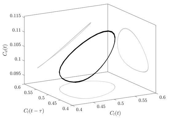
Figure 2.
Time-delay representation of the lift/drag coefficients with a .
It is possible to determine the lift and drag coefficients from the axial () and the transversal () force coefficients using the following relationship:
where is the angle of attack. From the inspection of Figure 2, it is possible to recognize the limit cycle behavior of the flow dynamics.
In Figure 3, panels (a) and (b) depict the contours of the time-averaged streamwise velocity component u and the transversal velocity component v.
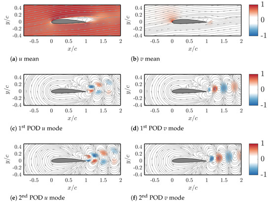
Figure 3.
Mean velocity fields and leading POD modes for a NACA 0012 at and . All field variables were normalized concerning their maximum.
These contour plots offer a visual representation of the mean flow characteristics. Panels (c) to (f) showcase the leading velocity modes within the POD framework. The first two modes, in particular, capture the most significant fluctuations in the flow field. It is important to note that the spatial shift in the direction of advection of the POD modes corresponds to the traveling pattern of the emitted eddies.
In Figure 4, velocity contour plots from three methods are compared: the FOM, POD−ROM with 10 velocity modes and 12 pressure and viscosity modes, and CNM−ROM using 10 clusters with a 4th-order model.
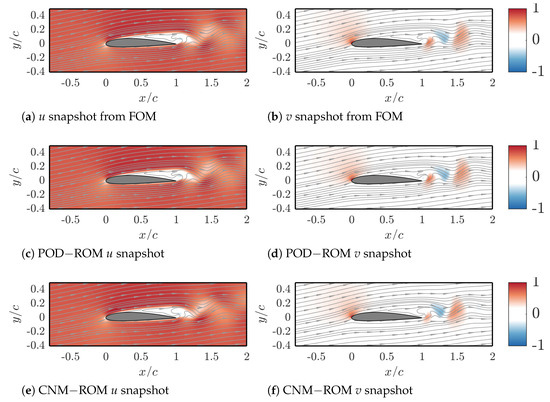
Figure 4.
Snapshots computed by FOM (first line), POD−ROM (second line), and CNM−ROM (third line). All field variables were normalized to their maximum.
This comparison is made at a specific time instant, second. This analysis allows us to assess the accuracy and fidelity of both the reduced-order models in capturing the flow features. The constructed flow fields obtained from the POD−ROM and CNM−ROM agree with the original FOM results, indicating the effectiveness of the reduced-order models in capturing the essential flow dynamics.
Figure 5 provides a comprehensive comparison of the axial and transversal force coefficients ( and ) obtained from the FOM, the POD−ROM, and the CNM−ROM at various ROM parameters.

Figure 5.
Force coefficients computed with FOM, POD−ROM, and CNM−ROM. In all the panels, the black lines refer to the FOM force coefficients. In panels (a,b), the blue lines correspond to the POD−ROM with 10 velocity modes and 12 pressure and viscosity modes; in panels (c,d), the red lines correspond to a first-order CNM−ROM, while the blue ones correspond to CNM−ROM with .
This comparison allows us to evaluate the accuracy and predictive capability of the reduced-order models in capturing the aerodynamic forces acting on the airfoil. The black lines represent the and coefficients obtained from the FOM simulations. In panels (a,b), the blue lines correspond to the and coefficients obtained from the POD−ROM, utilizing 10 velocity modes and 12 pressure and viscosity modes. In panels (c,d), the red lines correspond to the coefficients obtained from a first-order CNM−ROM, while the blue lines correspond to a fourth-order CNM−ROM. The figure demonstrates the capabilities of the CNM−ROM technique in accurately predicting the lift and drag coefficients, surpassing the performance of the POD−ROM. Therefore, the CNM−ROM approach (with a higher order) captures the complex flow phenomena more effectively, resulting in improved predictive accuracy of the aerodynamic forces.
To further analyze the statistical properties of the flow, the unbiased autocorrelation function between the FOM, POD−ROM, and CNM−ROM approaches is shown in Figure 6. The unbiased autocorrelation function (Protas et al. [36], Deng et al. [37]) is defined as follows:
where T is the simulation time and denotes the time delay, providing insights into the temporal correlation and persistence of flow features.
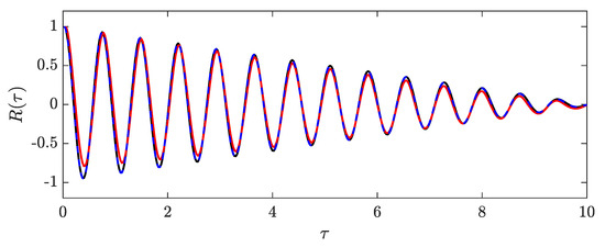
Figure 6.
Comparison of the autocorrelation function R between the FOM, POD−ROM, and CNM−ROM. The black line represents the FOM, the red line represents the POD−ROM, and the blue dashed line corresponds to the CNM−ROM.
Figure 6 demonstrates that the ROM approaches perform quite well in capturing the flow statistical properties and temporal correlations. However, the CNM−ROM exhibits a closer match to the autocorrelation function obtained from the FOM data, indicating its superior capability in reproducing the flow statistics.
When considering the first-order CNM, the direct transition probability matrix and the direct transition times matrix can be examined to describe the dynamics patterns. These matrices provide insights into how frequently and swiftly the system transitions between its various states or clusters. Figure 7 visually represents these matrices in panels (a) and (b), showcasing the direct transition probabilities () and times () of the CNM.
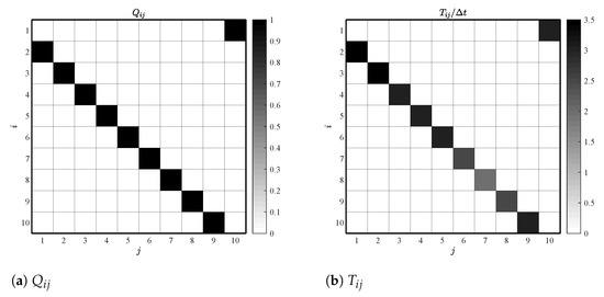
Figure 7.
The matrices for CNM direct transition probabilities () and times ().
Notably, the most likely transitions align with the subsequent clusters in the sequence, confirming the presence of a limit cycle in the system dynamics. Furthermore, by examining the transition times matrix, it is possible to estimate the dominant frequency by the following:
The versatility of the CNM−ROM approach becomes evident as it enables predictions of system behavior under various parameter and control configurations. In Figure 8, panel (a) illustrates the predictions for , while panel (b) depicts the predictions for when . These predictions are generated by training the CNM−ROM with snapshots from different values, excluding . This demonstrates the CNM−ROM’s ability to generalize the learned dynamics to unobserved parameter settings.
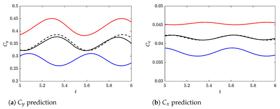
Figure 8.
Prediction of the effect of using CNM−ROM. The blue and red lines correspond to and , respectively. The black dashed lines represent the FOM simulations, while the black solid lines represent the CNM−ROM predictions.
Within Figure 8, the blue and red lines correspond to and , respectively. The black dashed lines represent the and coefficients obtained from the FOM simulations, and the black solid lines represent the predictions made by the CNM−ROM. Remarkably, the CNM−ROM accurately captures the amplitude and frequency of the force coefficients for varying values, including the unseen . This showcases the robustness and generalization capability of the CNM−ROM, as it effectively predicts the aerodynamic forces even for parameter values that were not included in its training data.
Overall, the results presented in this section validate the effectiveness of the POD−ROM and CNM−ROM approaches in accurately capturing the flow dynamics, reproducing the flow fields, predicting force coefficients, and capturing the statistical properties of the flow. These findings highlight the potential of reduced-order modeling techniques in enhancing computational efficiency and enabling rapid design iterations for airfoil configurations.
4. Conclusions
This study employs two distinct methodologies for analyzing the flow field over a NACA0012 airfoil at a moderate Reynolds number. The first methodology, the POD−ROM, involves truncating POD expansions for the velocity, pressure, and eddy viscosity fields to a reduced number of modes. The second methodology, the CNM−ROM, utilizes a directed network model, where coarse-grained states are represented as nodes. These reduced-order modeling frameworks offer the potential to design control strategies with significantly reduced computational demands compared to the full-order approach.
Numerical simulations for the full-order model were carried out using the OpenFOAM finite-volume solver. The proper orthogonal decomposition reduced-order model was implemented through the ITHACA-FV library within the OpenFOAM framework.
The comparative analysis of POD−ROM and CNM−ROM methodologies has revealed the superior effectiveness of CNM−ROM in accurately capturing flow dynamics and statistical characteristics while demanding fewer computational resources. The CNM−ROM approach, relying on direct transition matrices and cluster analysis, demonstrated its ability to provide precise flow field predictions and aerodynamic forces.
Furthermore, the CNM−ROM model showcased its versatility by successfully predicting the effect of varying flow parameters, such as the angle of attack. Training the CNM−ROM with snapshots from different angles of attack settings accurately captured the amplitude and frequency of the lift and drag coefficients for unseen angles of attack values. This demonstrates the robustness and generalization ability of the CNM−ROM approach.
The promising results obtained from both the POD−ROM and CNM−ROM methodologies underscore their potential applicability in determining optimal flow control configurations within the reduced-order modeling framework. These methodologies provide efficient alternatives for analyzing complex flow fields and have the potential to significantly reduce computational costs in aerodynamic design and optimization processes.
Author Contributions
Conceptualization, A.C. and E.D.C.; methodology, A.C.; software, E.D.C.; validation, A.C., M.C. and L.d.L.; formal analysis, A.C., M.C. and L.d.L.; investigation, A.C., M.C. and L.d.L.; resources, M.C. and L.d.L.; data curation, A.C., E.D.C., M.C. and L.d.L.; writing—original draft preparation, A.C.; writing—review and editing, A.C., E.D.C., M.C. and L.d.L.; visualization, A.C., E.D.C., M.C. and L.d.L.; supervision, M.C. and L.d.L.; project administration, M.C. and L.d.L. All authors have read and agreed to the published version of the manuscript.
Funding
This research received no external funding.
Institutional Review Board Statement
Not applicable.
Data Availability Statement
The data presented in this study are available upon request from the corresponding author.
Conflicts of Interest
The authors declare no conflicts of interest.
Abbreviations
The following abbreviations are used in this manuscript:
| URANS | unsteady Reynolds-averaged Navier–Stokes |
| FOM | full-order model |
| ROM | reduced-order model |
| POD | proper orthogonal decomposition |
| CNM | cluster-based network model |
References
- Couto, N.; Bergada, J.M. Aerodynamic Efficiency Improvement on a NACA-8412 Airfoil via Active Flow Control Implementation. Appl. Sci. 2022, 12, 4269. [Google Scholar] [CrossRef]
- Chiatto, M.; Palumbo, A.; de Luca, L. Design approach to predict synthetic jet formation and resonance amplifications. Exp. Therm. Fluid Sci. 2019, 107, 79–87. [Google Scholar] [CrossRef]
- Ceglia, G.; Chiatto, M.; Greco, C.S.; De Gregorio, F.; Cardone, G.; de Luca, L. Active control of separated flow over 2D back-facing ramp by an array of finite-span slotted synthetic jets. Exp. Therm. Fluid Sci. 2021, 129, 110475. [Google Scholar] [CrossRef]
- Girfoglio, M.; Greco, C.; Chiatto, M.; de Luca, L. Modelling of efficiency of synthetic jet actuators. Sens. Actuators A Phys. 2015, 233, 512–521. [Google Scholar] [CrossRef]
- de Luca, L.; Girfoglio, M.; Chiatto, M.; Coppola, G. Scaling properties of resonant cavities driven by piezo-electric actuators. Sens. Actuators A Phys. 2016, 247, 465–474. [Google Scholar] [CrossRef]
- Tousi, N.; Coma, M.; Bergadà, J.; Pons-Prats, J.; Mellibovsky, F.; Bugeda, G. Active flow control optimisation on SD7003 airfoil at pre and post-stall angles of attack using synthetic jets. Appl. Math. Model. 2021, 98, 435–464. [Google Scholar] [CrossRef]
- Tousi, N.; Bergadà, J.; Mellibovsky, F. Large Eddy Simulation of optimal Synthetic Jet Actuation on a SD7003 airfoil in post-stall conditions. Aerosp. Sci. Technol. 2022, 127, 107679. [Google Scholar] [CrossRef]
- Lahey, R.; Cheng, L.; Drew, D.; Flaherty, J. The effect of virtual mass on the numerical stability of accelerating two-phase flows. Int. J. Multiph. Flow 1980, 6, 281–294. [Google Scholar] [CrossRef]
- Li, Y.; Cui, W.; Jia, Q.; Li, Q.; Yang, Z.; Morzyński, M.; Noack, B.R. Explorative gradient method for active drag reduction of the fluidic pinball and slanted Ahmed body. J. Fluid Mech. 2022, 932, A7. [Google Scholar] [CrossRef]
- Reumschüssel, J.M.; von Saldern, J.G.R.; Li, Y.; Paschereit, C.O.; Orchini, A. Gradient-Free Optimization in Thermoacoustics: Application to a Low-Order Model. J. Eng. Gas Turbines Power 2022, 144, 051004. [Google Scholar] [CrossRef]
- Wang, T.; Yang, Y.; Chen, X.; Li, P.; Iollo, A.; Maceda, G.Y.C.; Noack, B.R. Topologically assisted optimization for rotor design. Phys. Fluids 2023, 35, 055105. [Google Scholar] [CrossRef]
- Taira, K.; Brunton, S.L.; Dawson, S.T.M.; Rowley, C.W.; Colonius, T.; McKeon, B.J.; Schmidt, O.T.; Gordeyev, S.; Theofilis, V.; Ukeiley, L.S. Modal Analysis of Fluid Flows: An Overview. AIAA J. 2017, 55, 4013–4041. [Google Scholar] [CrossRef]
- Rowley, C.W.; Dawson, S.T. Model Reduction for Flow Analysis and Control. Annu. Rev. Fluid Mech. 2017, 49, 387–417. [Google Scholar] [CrossRef]
- Schmid, P. Dynamic Mode Decomposition and Its Variants. Annu. Rev. Fluid Mech. 2022, 54, 225–254. [Google Scholar] [CrossRef]
- Herrmann, B.; Baddoo, P.J.; Semaan, R.; Brunton, S.L.; McKeon, B.J. Data-driven resolvent analysis. J. Fluid Mech. 2021, 918, A10. [Google Scholar] [CrossRef]
- Schmidt, S.; Oberleithner, K. Global modes of variable-viscosity two-phase swirling flows and their triadic resonance. J. Fluid Mech. 2023, 955, A24. [Google Scholar] [CrossRef]
- Stabile, G.; Hijazi, S.; Mola, A.; Lorenzi, S.; Rozza, G. POD-Galerkin reduced order methods for CFD using Finite Volume Discretisation: Vortex shedding around a circular cylinder. Commun. Appl. Ind. Math. 2017, 8, 210–236. [Google Scholar] [CrossRef]
- Noack, B.R.; Afanasiev, K.; Morzyński, M.; Tadmor, G.; Thiele, F. A hierarchy of low-dimensional models for the transient and post-transient cylinder wake. J. Fluid Mech. 2003, 497, 335–363. [Google Scholar] [CrossRef]
- Noack, B.; Morzynski, M.; Tadmor, G. Reduced-Order Modelling for Flow Control; Springer: Vienna, Austria, 2011. [Google Scholar] [CrossRef]
- Taira, K.; Hemati, M.S.; Brunton, S.L.; Sun, Y.; Duraisamy, K.; Bagheri, S.; Dawson, S.T.M.; Yeh, C. Modal Analysis of Fluid Flows: Applications and Outlook. AIAA J. 2020, 58, 998–1022. [Google Scholar] [CrossRef]
- Racca, A.; Magri, L. Data-driven prediction and control of extreme events in a chaotic flow. Phys. Rev. Fluids 2022, 7, 104402. [Google Scholar] [CrossRef]
- Fernex, D.; Noack, B.R.; Semaan, R. Cluster-based network modeling—From snapshots to complex dynamical systems. Sci. Adv. 2021, 7, eabf5006. [Google Scholar] [CrossRef] [PubMed]
- Hou, C.; Deng, N.; Noack, B.R. Trajectory-optimized cluster-based network model for the sphere wake. Phys. Fluids 2022, 34. [Google Scholar] [CrossRef]
- Colanera, A.; Reumschüssel, J.M.; Beuth, J.P.; Chiatto, M.; de Luca, L.; Oberleithner, K. Extended Cluster-Based Network Modeling for Coherent Structures in Turbulent Flows. 2023. Available online: https://www.researchsquare.com/article/rs-3788637/v1 (accessed on 23 January 2024). [CrossRef]
- Wang, X.; Deng, N.; Maceda, G.Y.C.; Noack, B.R. Cluster-based control for net drag reduction of the fluidic pinball. Phys. Fluids 2023, 35, 023601. [Google Scholar] [CrossRef]
- Brunton, S.L.; Noack, B.R.; Koumoutsakos, P. Machine Learning for Fluid Mechanics. Annu. Rev. Fluid Mech. 2020, 52, 477–508. [Google Scholar] [CrossRef]
- Saetta, E.; Tognaccini, R.; Iaccarino, G. Machine Learning to Predict Aerodynamic Stall. Int. J. Comput. Fluid Dyn. 2022, 36, 641–654. [Google Scholar] [CrossRef]
- Stabile, G.; Rozza, G. Finite volume POD-Galerkin stabilised reduced order methods for the parametrised incompressible Navier-Stokes equations. Comput. Fluids 2018, 173, 273–284. [Google Scholar] [CrossRef]
- Kaiser, E.; Noack, B.R.; Cordier, L.; Spohn, A.; Segond, M.; Abel, M.; Daviller, G.; Östh, J.; Krajnović, S.; Niven, R.K.; et al. Cluster-based reduced-order modelling of a mixing layer. J. Fluid Mech. 2014, 754, 365–414. [Google Scholar] [CrossRef]
- Li, H.; Fernex, D.; Semaan, R.; Tan, J.; Morzyński, M.; Noack, B.R. Cluster-based network model. J. Fluid Mech. 2021, 906, A21. [Google Scholar] [CrossRef]
- Di Costanzo, E.; Colanera, A.; Chiatto, M.; de Luca, L. Cluster-based network reduced order modeling for flow fields around airfoil profiles. In Proceedings of the AIAA AVIATION 2023 Forum, San Diego, CA, USA, 12–16 June 2023; American Institute of Aeronautics and Astronautics: Reston, VA, USA, 2023. [Google Scholar] [CrossRef]
- Hijazi, S.; Stabile, G.; Mola, A.; Rozza, G. Data-driven POD-Galerkin reduced order model for turbulent flows. J. Comput. Phys. 2020, 416, 109513. [Google Scholar] [CrossRef]
- Ballarin, F.; Manzoni, A.; Quarteroni, A.; Rozza, G. Supremizer stabilization of POD-Galerkin approximation of parametrized steady incompressible Navier-Stokes equations. Int. J. Numer. Methods Eng. 2015, 102, 1136–1161. [Google Scholar] [CrossRef]
- MacQueen, J.B. Some methods for classification and analysis of multivariate observations. Berkeley Symp. Math. Statist. Prob. 1967, 1, 281–297. [Google Scholar]
- Lloyd, S.P. Least Squares Quantization in PCM. IEEE Trans. Inf. Theory 1982, 28, 129–137. [Google Scholar] [CrossRef]
- Protas, B.; Noack, B.R.; Östh, J. Optimal nonlinear eddy viscosity in Galerkin models of turbulent flows. J. Fluid Mech. 2015, 766, 337–367. [Google Scholar] [CrossRef]
- Deng, N.; Noack, B.R.; Morzyński, M.; Pastur, L.R. Cluster-based hierarchical network model of the fluidic pinball–Cartographing transient and post-transient, multi-frequency, multi-attractor behaviour. J. Fluid Mech. 2022, 934, A24. [Google Scholar] [CrossRef]
Disclaimer/Publisher’s Note: The statements, opinions and data contained in all publications are solely those of the individual author(s) and contributor(s) and not of MDPI and/or the editor(s). MDPI and/or the editor(s) disclaim responsibility for any injury to people or property resulting from any ideas, methods, instructions or products referred to in the content. |
© 2024 by the authors. Licensee MDPI, Basel, Switzerland. This article is an open access article distributed under the terms and conditions of the Creative Commons Attribution (CC BY) license (https://creativecommons.org/licenses/by/4.0/).