Research on the Mechanical Parameter Identification and Controller Performance of Permanent Magnet Motors Based on Sensorless Control

Abstract

In order to improve the control performance of the position sensorless control system of permanent magnet synchronous motors and to reduce the influence of external uncertainties on the control system, such as inertia ingestion and load disturbance, this paper proposes a novel position sensorless control algorithm for permanent magnet synchronous motors based on an interleaved parallel extended sliding mode observer. Firstly, in order to identify the time-varying moment of inertia, load torque and viscous friction coefficient of the system, a novel interleaved parallel extended sliding mode observer based on a single-observer model is proposed, and a robust activator is designed to reduce the coupling between the parameters to be measured. Then, a new predefined-time sliding mode controller is designed for the face-mounted permanent magnet synchronous motor using sliding film control theory, which improves the response speed and control accuracy of the system. Then, the proposed novel interleaved parallel extended sliding mode observer and predefined-time sliding mode controller are used to design the permanent magnet synchronous motor control system, and the stability of the system is proved using the Lyapunov stability theorem. Finally, through simulation analysis and experimental tests, it is verified that the control strategy proposed in this paper can improve the identification accuracy of the motor parameters, reduce the time of identification, and improve the control accuracy and tracking speed.

1. Introduction

Permanent Magnet Synchronous Motors (PMSMs) have the advantages of high efficiency, small size, low loss, simple structure, reliable operation, etc., and have been more and more widely used in the field of hybrid vehicles, numerical control machine tools, wind power generation and so on. With the development of society, the requirements for motor control accuracy in different working environments are becoming higher and higher [1,2]. As the internal parameters of the motor will constantly change with the external environment, load changes and other factors during the operation of the motor, this, in turn, will lead to a decline in the performance of the control system. Therefore, the control system is required to be able to accurately identify the parameters of the motor system and adjust the control strategy at the right time to meet the performance requirements of the production machinery on the motor control system [3].

The research on control strategy includes two parts: the system state observer and the design of the controller. Scholars at home and abroad have conducted extensive research on the study of motor control system state observers and proposed many algorithms. These include stepwise estimation based on a Sliding Mode Observer [4,5,6], Extended Kalman Filter (EKF) [7,8,9], Model Reference Adaptive Control (MRAC) [10,11], Recursive Least Squares (Recursive Least Squares (RLS) [12,13,14] and Algebraic Parameter Identification (API) [15,16], among others. The authors of [17] extracted three parameters (moment of inertia, load torque and the viscous friction coefficient) from the perturbations observed by a higher-order Sliding Mode Observer (SMO) using a three-step method; [18] similarly extracted the same three mechanical parameters from an Extended Sliding Mode Observer (ESMO) using a three-step method. Although the algorithms used in [17,18] are capable of extracting the mechanical parameters of the motor, the extraction process has to be carried out in three steps, which makes the extraction process complex and has limitations in practical applications (e.g., in the field of industrial robotics where both the moment of inertia and load torque are time-varying). Although ref. [19] achieved the simultaneous identification of multiple mechanical parameters, the complex matrix operations of the algorithm greatly increase the difficulty of the controller hardware design. Both refs. [20,21] used recursive least squares and algebraic parameter identification methods to identify each mechanical parameter online, respectively, but problems remain of high matrix complexity, excessive computation of the algorithm and poor system robustness.

In terms of motor control algorithms, traditional vector PI control can no longer meet higher control requirements, so scholars have proposed a series of control algorithms, such as Sliding Mode Control (SMC) [22,23], Passivity-based Control (PBC) [24], Robust Control (RC) [25,26,27], Fuzzy Logic Control (FLC) [28,29,30], and Model-Free Adaptive Control (MFAC) [31,32]. The authors of [33] proposed an adaptive terminal sliding mode control algorithm for the speed tracking control problem of motors, which has both adaptive switching inputs and FO integral sliding mode surfaces, greatly reducing the dependence of the control algorithm on system parameters. Ref. [34] proposed a novel discrete-time multi-stage sliding mode control algorithm to provide good speed tracking performance of the motor system under different operating conditions. In ref. [35], the authors reduced the effect of load disturbances on the performance of the motor system using a fractional-order composite integral sliding mode control algorithm. The above algorithm only improves the motor control system and minimises the effects of parameter perturbations and changes in the operating environment on the control system, and does not adopt a control strategy that combines an observer and a controller. Ref. [36] used an improved recursive least squares method to identify the motor parameters and ensure the dynamic performance of the motor under different operating conditions, but the algorithm still suffers from the problem of excessive computation, and only identifies the parameters of the motor, and does not feed back the identification results to the control system.

In this paper, a novel position sensorless control system for permanent magnet synchronous motors is designed based on an interleaved parallel extended sliding mode observer and a predefined-time sliding mode controller. The paper makes the following main contributions:

(1)

A new Predefined-Time Sliding Mode Controller (NPTSMC) is proposed. Firstly, the basic model of the controller is analyzed by means of multi-parameter definition; then, a new sliding mode surface is designed based on the model and a new sliding mode controller is investigated to improve the control accuracy and convergence speed of the system.

(2)

A new Interleaved Parallel Extended Sliding Mode Observer (IPESMO) capable of observing three system variables simultaneously is proposed. Each of the three mechanical parameters is first expanded into a new system state variable, and then a simultaneous estimation of the system state is performed using the expanded observer. During the observer design process, a time-varying feedback gain is incorporated into each of the novel observers, and this design improves the accuracy of the observation error and the speed of convergence. Furthermore, the novel interleaved parallel extended sliding mode observer designed in this paper greatly reduces the complexity of matrix computation and has the property of being a Low Pass Filter (LPF), which enables the system to output smooth estimation results even at high switching gains.

(3)

Combining three novel extended sliding mode observers into one interleaved parallel interconnected observer for simultaneous multi-parameter estimation. While effectively reducing the system complexity, this also improves the observation efficiency.

(4)

A robust activator is designed to reduce the coupling effect between the parameters to be measured and is combined with the observer as a Robust Activator Interleaved Parallel Extended Sliding Mode Observer (RAIPESMO) with a robust activator. Firstly, the coupled error equations are established and the mathematical model of each to-be-measured value is analyzed based on the to-be-measured parameter model; then, the neglected effects are eliminated from the model; finally, the robust activator is simplified to an observer gain parameter with a decoupling function. This design can improve the problems of reduced observation accuracy and long convergence time caused by parameter coupling effects during the operation of the observer.

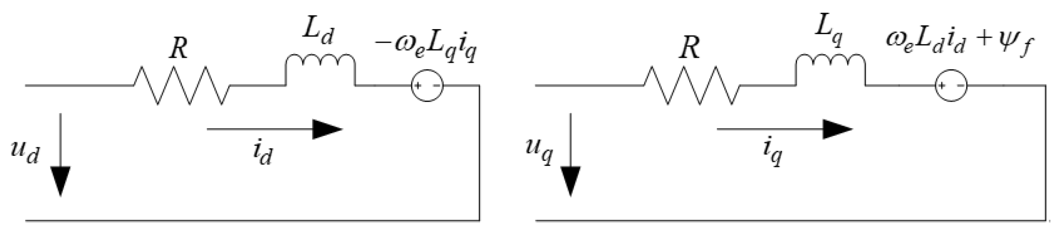
2. Mathematical Models of Surface-Mounted Permanent Magnet Synchronous Motors

The stator voltage equation for the d-q axis of the synchronous rotating coordinate system of a surface-mounted permanent magnet synchronous motor is given by:

$$\left\{\begin{array}{c}{u}_d=R{i}_d+L_d{\displaystyle \frac{d}{dt}}{i}_d-{\omega }_e{L}_q{i}_q\hfill \\ u_q=R{i}_q+L_q{\displaystyle \frac{d}{dt}}{i}_q+{\omega }_e\left(L_d{i}_d+{\psi }_f\right)\hfill \end{array}\right.$$

(1)

where $u_d$ and $u_q$ are the $\mathit{d}$-$\mathit{q}$ axis components of the stator voltage, respectively; $i_d$ and $i_q$ are the $\mathit{d}$-$\mathit{q}$ axis components of the stator current, respectively; R is the stator resistance; ${\omega }_e$ is the electrical angular speed; $L_d$ and $L_q$ are the $\mathit{d}$-$\mathit{q}$ axis inductive components, respectively; and ${\psi }_f$ is the rotor permanent-magnet flux linkage.

The voltage equivalent circuit shown in Figure 1 can be obtained from Equation (1).

At this point, the electromagnetic torque equation is:

$$T_e={\displaystyle \frac{3}{2}}{p}_n{i}_q\left[i_d\left(L_d-L_q\right)+{\psi }_f\right]$$

(2)

where $p_n$ is the number of pole pairs of the permanent magnet synchronous motor.

For the surface-mounted permanent magnet synchronous motor, the stator inductance satisfies $L_d$ = $L_q$, so the electromagnetic torque equation can be rewritten as Equation (3):

$$T_e={\displaystyle \frac{3}{2}}{p}_n{i}_q{\psi }_f=K_T{i}_q$$

(3)

In addition, the mechanical equationsof motion for the PMSM is:

$$J{\displaystyle \frac{d{\omega }_m}{dt}}=T_e-T_l-T_L$$

(4)

where ${\omega }_m$ is the mechanical angular velocity of the motor; $\mathit{J}$ is the moment of inertia; $T_L$ is the load torque; and $T_l$ is the friction torque.

When calculating the friction torque of a permanent magnet synchronous motor, the expression for ${\widehat{T}}_l$ is:

$$\widehat{T_l}=g_1{\omega }_m^2+g_2{\omega }_m+g_{3}sign\left({\omega }_m\right)$$

(5)

where $g_1$, $g_2$ and $g_3$ will be obtained by curve fitting under no-load-torque steady-state tests. In most of the current studies, $g_2$ is considered as a constant value and $g_3$ is ignored.

The relational equations for the rest of the parameters in this paper are as follows:

$$\left\{\begin{array}{c}{\omega }_e=n_p{\omega }_m\hfill \\ N_r={\displaystyle \frac{30}{\pi }}{\omega }_m\hfill \\ {\theta }_e=\int {\omega }_{e}dt\hfill \\ \overline{N}={\widehat{N}}_r-N_r\hfill \end{array}\right.$$

(6)

where $N_r$, ${\widehat{N}}_r$ and $\widehat{N}$ are the actual speed of the motor, the estimated speed of the motor and the motor speed error, respectively.

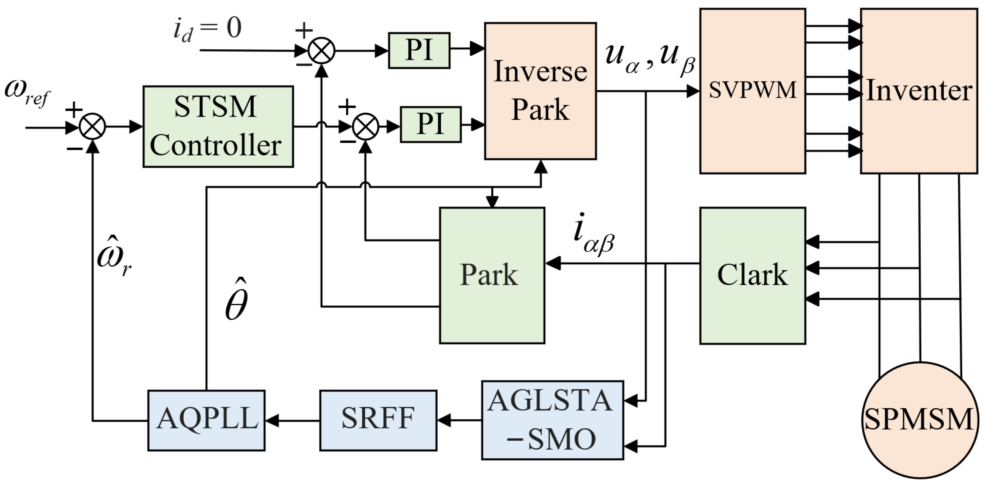
3. New Predefined-Time Sliding Mode Control Scheme

3.1. System Description

Consider a drive system response system with internal uncertainties and external disturbances:

$$\left\{\begin{array}{c}\dot{x}=f(x,t)+\Delta f(x,t)+n\left(t\right)\hfill \\ \dot{y}=g(y,t)+\Delta g(y,t)+m\left(t\right)+u\left(t\right)\hfill \end{array}\right.$$

(7)

where $\mathit{x}$, $\mathit{y}$ is the system response; $f(x,t)$ and $g(y,t)$ are the smoothing functions; $\Delta f(x,t)$ and $\Delta g(y,t)$ are the internal errors of the model; $n\left(t\right)$ and $m\left(t\right)$ are the external perturbations; and $u\left(t\right)$ is the controller input.

In performing the controller analysis, we assume that both the internal errors and external perturbations of the system are bounded.

$$∥\Delta f\left(x\right)∥\le A∥x∥,∥\Delta g\left(y\right)∥\le B∥y∥∥n\left(t\right)∥\le C,∥m\left(t\right)∥\le D$$

(8)

where $∥·∥$ is the Euclidean paradigm; $\mathit{A}$, $\mathit{B}$, $\mathit{C}$ and $\mathit{D}$ are constants. The system error equation can be obtained from Equation (7):

$$\dot{e}=g(y,t)-f(x,t)+\Delta g(y,t)-\Delta f(x,t)+m\left(t\right)-n\left(t\right)+u\left(t\right)$$

(9)

In order to prove the convergence of the sliding mode surface and the stability of the sliding mode controller, Theorem 1 is introduced here.

Theorem 1.

For any constant $\mathit{T}$ greater than zero, system $\dot{x}\left(t\right)=\varphi (t,x)$ is predefined-time stable if the system $\dot{x}\left(t\right)=\varphi (t,x)$ has an unbounded Lyapunov function $V\left(x\right)$ satisfying Equation (10).

$$\dot{V}\le -{\displaystyle \frac{1}{T}}{\displaystyle \frac{2}{\alpha }}\left(2V+V^{1-\alpha /2}+V^{1+\alpha /2}\right)$$

(10)

where $\mathit{T}$ is a predefined time set by the system and $\alpha \in (0,1)$.

When the predefined-time controller is used, if the value of time $\mathit{T}$ is predetermined, the controller will automatically adjust the convergence time of the system to meet the requirements of the predefined-time control. Equation (10) is considered as a Lyapunov sufficient condition for the new predefined-time controller.

Proof of Theorem 1 .

$$\begin{array}{cc}\hfill T\left(x\right)& \le T{\displaystyle \frac{\alpha }{2}}{\displaystyle \frac{dV}{2V+V^{1-\alpha /2}+V^{1+\alpha /2}}}\hfill \\ \hfill & =-T{\displaystyle \frac{\alpha }{2}}{\int }_{V_0}^{V_{t_f}}{\displaystyle \frac{dV}{V^{1-\alpha /2}{\left(1+V^{\alpha /2}\right)}^2}}\hfill \\ \hfill & =-T{\displaystyle \frac{\alpha }{2}}{\int }_{V_0}^{V_{t_f}}{\displaystyle \frac{d{V}^{\alpha /2}}{{\left(1+V^{\alpha /2}\right)}^2}}\hfill \\ \hfill & =T{\displaystyle \frac{\alpha }{\pi }}{\displaystyle \frac{2}{\alpha }}{\int }_0^{V_0}{\displaystyle \frac{d{V}^{\alpha /2}}{\left(1+V^{\alpha }\right)}}\hfill \\ \hfill & =T\left(1-{\left(1+V_0^{\alpha /2}\right)}^{-1}\right)\hfill \\ \hfill & \le T\hfill \end{array}$$

(11)

From Equation (11), it can be concluded that the system will converge in a predefined time when $T\left(x\right)\le T$. □

3.2. Designing a New Sliding Mode Surface

To enable the error system to reach a steady state in a predefined time, the sliding mode surface is designed:

$$s=\overline{N}+{\int }_0^t\left(a_1\overline{N}+a_{2}sign\left(\overline{N}\right){\left|\overline{N}\right|}^{1-\alpha }+a_{3}sign\left(\overline{N}\right){\left|\overline{N}\right|}^{1+\alpha }+a_{4}sign\left(\overline{N}\right)\right)d\tau$$

(12)

where $a\in (0,1),a_1={\displaystyle \frac{2}{T_1\alpha }},a_2={\displaystyle \frac{2}{T_1\alpha }}{\left({\displaystyle \frac{1}{2}}\right)}^{1-\alpha /2},a_3={\displaystyle \frac{2}{T_1\alpha }}{\left({\displaystyle \frac{1}{2}}\right)}^{1+\alpha /2},a_4>0$.

If Equation (12) is the system error, the system will converge to zero on the sliding mode surface in a predefined time $T_1$.

Convergence Proof: When the error system is moving on the sliding mode surface, it satisfies $S\left(t\right)=\left\{\begin{array}{c}\overline{N}|s\left(\overline{N}\right)=0\end{array}\right\}$ and $\dot{s}\left(\overline{N}\right)=0$, Equation (13) can be obtained:

$$\dot{\overline{N}}=-\left(a_1\overline{N}+a_{2}sign\left(\overline{N}\right){\left|\overline{N}\right|}^{1-\alpha }+a_{3}sign\left(\overline{N}\right){\left|\overline{N}\right|}^{1+\alpha }+a_{4}sign\left(\overline{N}\right)\right)$$

(13)

Selecting $V={\displaystyle \frac{1}{2}}{\overline{N}}^2$ as the Lyapunov function of the system, it can be found:

$$\begin{array}{cc}\hfill \dot{V}& =\widehat{N}·\widehat{N}\hfill \\ \hfill & =-\overline{N}\left(a_1\overline{N}+a_{2}sign\left(\overline{N}\right)|\overline{N}{|}^{1-\alpha }+a_{3}sign\left(\overline{N}\right)|\overline{N}{|}^{1+\alpha }+a_{4}sign\left(\overline{N}\right)\right)\hfill \\ \hfill & =-\left(a_1{\overline{N}}^2+a_2{\left|\overline{N}\right|}^{2-\alpha }+a_3{\left|\overline{N}\right|}^{2+\alpha }+a_4\left|\overline{N}\right|\right)\hfill \\ \hfill & \le -\left(a_1{\overline{N}}^2+a_2{\left|\overline{N}\right|}^{2-\alpha }+a_3{\left|\overline{N}\right|}^{2+\alpha }\right)\hfill \\ \hfill & \le -{\displaystyle \frac{1}{T_1}}{\displaystyle \frac{2}{\alpha }}\left(2V+V^{1-\alpha /2}+V^{1+\alpha /2}\right)\hfill \end{array}$$

(14)

After the above analysis, it can be shown that Equation (14) satisfies the predefined time stability theorem, which proves that the error system will converge to zero within a predefined time $T_1$.

3.3. New Predefined-Time Sliding Mode Controller

In order to satisfy the definition of the predefined time control of the system, Equation (12) is used as the sliding mode surface of the system, at which point, the controller can be designed as:

$$\begin{array}{cc}& u=f\left(x\right)-g\left(y\right)-\left(a_1\overline{N}+a_{2}sign\left(\overline{N}\right)|\overline{N}{|}^{1-\alpha }+a_{3}sign\left(\overline{N}\right)|\overline{N}{|}^{1+\alpha }+a_{4}sign\left(\overline{N}\right)\right)\hfill \\ & -\left(a_{5}s+a_{6}sign\left(s\right)|s{|}^{1-\alpha }+a_{7}sign\left(s\right)|s{|}^{1+\alpha }+a_{8}sign\left(s\right)\right)-\left(A∥x∥+B∥y∥+C+D\right)sign\left(s\right)\hfill \end{array}$$

(15)

where $a_5={\displaystyle \frac{2}{T_2\alpha }},a_6={\displaystyle \frac{2}{T_2\alpha }}{\left({\displaystyle \frac{1}{2}}\right)}^{1-\alpha /2},a_7={\displaystyle \frac{2}{T_2\alpha }}{\left({\displaystyle \frac{1}{2}}\right)}^{1+\alpha /2},a_8>0$.

If Equation (15) is used as a controller function for the error system, the system will arrive at the sliding mode surface within a predefined time $T_2$.

Stability proof: Choice $V={\displaystyle \frac{1}{2}}{s}^2$ is the Lyapunov function, which is proved as follows:

$$\begin{array}{cc}\hfill \mathrm{V}& =s·\dot{s}=s\left(\dot{N}+a_1\overline{N}+a_{2}sign\left(\overline{N}\right)|\overline{N}{|}^{1-\alpha }+a_{3}sign\left(\overline{N}\right)|\overline{N}{|}^{1+\alpha }+a_{4}sign\left(\overline{N}\right)\right)\hfill \\ \hfill & =s\left(\left(g\left(y\right)+\Delta g\left(y\right)+n+u-\left(f\left(x\right)+\Delta f\left(x\right)+m\right)\right)\right)+s\left(a_1\overline{N}+a_{2}sign\left(\overline{N}\right)|\overline{N}{|}^{1-\alpha }+a_{3}sign\left(\overline{N}\right)|\overline{N}{|}^{1+\alpha }+a_{4}sign\left(\overline{N}\right)\right)\hfill \\ \hfill & =s\left(\Delta g\left(y\right)+m-\left(\Delta f\left(x\right)+n\right)\right)-\left|s\right|\left(A\parallel x\parallel +B\parallel y\parallel +C+D\right)-s\left(a_{5}s+a_{6}sign\left(s\right)|s{|}^{1-\alpha }+a_{7}sign\left(s\right)|s{|}^{1+\alpha }+a_{8}sign\left(s\right)\right)\hfill \\ \hfill & =-\left(a_5{s}^2+a_6{\left|s\right|}^{2-\alpha }+a_7{\left|s\right|}^{2+\alpha }+a_8\left|s\right|\right)\hfill \\ \hfill & \le -{\displaystyle \frac{1}{T_2}}{\displaystyle \frac{2}{\alpha }}\left(2V+V^{1-\alpha /2}+V^{1+\alpha /2}\right)\hfill \end{array}$$

(16)

It can be shown that Equation (16) satisfies Theorem 1. It is concluded that the error system will reach the sliding mode surface within a predefined time $T_2$.

In summary, when Equations (12) and (15) are used as the sliding mode surface and controller of the control system, respectively, the system error converges to 0 in a predefined time, which is the predefined-time sliding mode control scheme proposed in this paper.

In this paper, the control method with id = 0 is used to estimate the rotor information using the finite time super-helical sliding mode observer algorithm, and the control framework of this paper is shown in Figure 2.

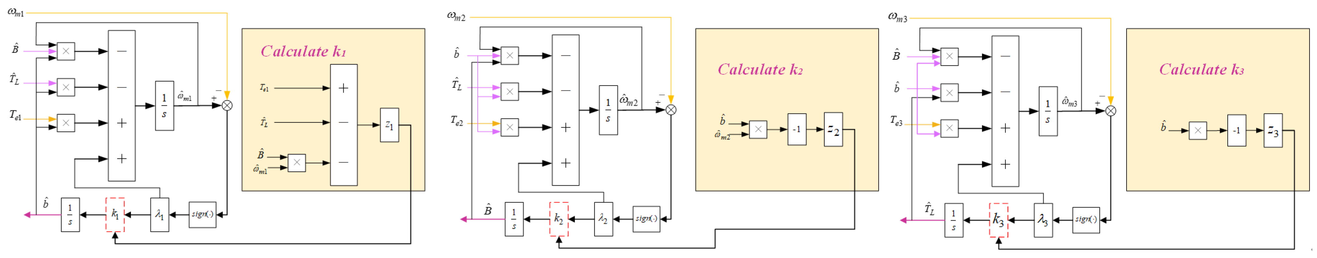
4. Interleaved Parallel Extended Sliding Mode Observer

4.1. Establishment of Mechanical Equations of Motion for Permanent Magnet Synchronous Motors

In order to simplify the analysis process, three equations of mechanical motion of permanent magnet synchronous motors are established, and the moment of inertia, viscous friction coefficient and load torque are expressed separately.

$$\begin{array}{c}\mathrm{System}1:\left\{\begin{array}{c}{\dot{\omega }}_{m1}=b\left(T_{e1}-T_L-B{\omega }_{m1}\right)\hfill \\ \dot{b}=r_1\hfill \end{array}\right.\\ \mathrm{System}2:\left\{\begin{array}{c}{\dot{\omega }}_{m2}=b\left(T_{e2}-T_L-B{\omega }_{m2}\right)\hfill \\ \dot{B}=r_2\hfill \end{array}\right.\\ \mathrm{System}3:\left\{\begin{array}{c}{\dot{\omega }}_{m3}=b\left(T_{e3}-T_L-B{\omega }_{m3}\right)\hfill \\ {\dot{T}}_L=r_3\hfill \end{array}\right.\end{array}$$

(17)

where $\mathit{b}$ = 1/$\mathit{J}$; $r_1$, $r_2$ and $r_3$ are the derivatives of $\mathit{b}$, $\mathit{B}$ and $T_L$ with respect to time, respectively.

4.2. Design of a Parallel Doubly Extended Sliding Mode Observer

Based on the extended sliding mode observer algorithm, the novel extended sliding mode observer systems 1, 2 and 3 are designed in this paper. ${\omega }_{mi}$ and $\mathit{b}$ are taken as the observation objects of the system to estimate the moment of inertia $\mathit{J}$, the viscous friction coefficient $\mathit{B}$ and the load torque $T_L$; thus, the observers are designed as follows:

$$\begin{array}{c}\mathrm{Observer}1:\left\{\begin{array}{c}{\dot{\widehat{\omega }}}_{m1}=\widehat{b}\left(T_{e1}-{\widehat{T}}_L-\widehat{B}{\widehat{\omega }}_{m1}\right)+{\lambda }_{1}sign\left(S_1\right)\hfill \\ \dot{\widehat{b}}=Q_1\hfill \end{array}\right.\\ \mathrm{Observer}2:\left\{\begin{array}{c}{\dot{\widehat{\omega }}}_{m2}=\widehat{b}\left(T_{e2}-{\widehat{T}}_L-\widehat{B}{\widehat{\omega }}_{m2}\right)+{\lambda }_{2}sign\left(S_2\right)\hfill \\ \dot{\widehat{B}}=Q_2\hfill \end{array}\right.\\ \mathrm{Observer}3:\left\{\begin{array}{c}{\dot{\widehat{\omega }}}_{m3}=\widehat{b}\left(T_{e3}-{\widehat{T}}_L-\widehat{B}{\widehat{\omega }}_{m3}\right)+{\lambda }_{3}sign\left(S_3\right)\hfill \\ {\dot{\widehat{T}}}_L=Q_3\hfill \end{array}\right.\end{array}$$

(18)

where ${\widehat{\omega }}_{m1}$, ${\widehat{\omega }}_{m2}$, ${\widehat{\omega }}_{m3}$, $\widehat{b}$, $\widehat{B}$, ${\widehat{T}}_L$ are the estimated values of ${\omega }_{m1}$, ${\omega }_{m2}$, ${\omega }_{m3}$, $\mathit{b}$, $\mathit{B}$, $T_L$, respectively; ${\lambda }_1$, ${\lambda }_2$, ${\lambda }_3$ are the switching function gains; $S_i$ and $Q_i$ are the derivatives of the sliding mode surface and the values to be observed, respectively.

The mechanical angular velocity of the motor can be derived from the sensorless observation algorithm. The following parameters are further defined:

$$\left\{\begin{array}{c}{e}_{11}={\widehat{\omega }}_{m1}-{\omega }_{m1}\hfill \\ e_{12}=\widehat{b}-b\hfill \\ e_{21}={\widehat{\omega }}_{m2}-{\omega }_{m2}\hfill \\ e_{22}=\widehat{B}-B\hfill \\ e_{31}={\widehat{\omega }}_{m3}-{\omega }_{m3}\hfill \\ e_{32}={\widehat{T}}_L-T_L\hfill \end{array}\right.$$

(19)

Subtracting Equation (18) from Equation (17) gives the error equation for the observer as:

$$\begin{array}{c}\mathrm{Error}1:\left\{\begin{array}{c}{\dot{e}}_{11}=e_{12}\left(T_{e1}-{\widehat{T}}_L-\widehat{B}{\widehat{\omega }}_{m1}\right)-b\left(\widehat{B}{e}_{11}+e_{32}+{\omega }_{m1}{e}_{22}\right)+{\lambda }_{1}sign\left(S_1\right)\hfill \\ {\dot{e}}_{12}=Q_1-r_1\hfill \end{array}\right.\\ \mathrm{Error}2:\left\{\begin{array}{c}{\dot{e}}_{21}=e_{12}\left(T_{e2}-T_L-B{\omega }_{m2}\right)-\widehat{b}\left({\widehat{\omega }}_{m2}{e}_{22}+B{e}_{21}+e_{32}\right)+{\lambda }_{2}sign\left(S_2\right)\hfill \\ {\dot{e}}_{22}=Q_2-r_2\hfill \end{array}\right.\\ \mathrm{Error}3:\left\{\begin{array}{c}{\dot{e}}_{31}=e_{12}\left(T_{\mathbf{e}3}-T_L-B{\omega }_{\mathbf{m}3}\right)-\widehat{b}\left(e_{32}+B{e}_{31}+{\widehat{\omega }}_{\mathbf{m}3}{e}_{22}\right)+{\lambda }_{3}sign\left(S_3\right)\hfill \\ {\dot{e}}_{32}=Q_3-r_3\hfill \end{array}\right.\end{array}$$

(20)

When the observer analysis is performed, variables $T_{e1}-{\widehat{T}}_L-\widehat{B}{\widehat{\omega }}_{m1}$, $b\left(\widehat{B}{e}_{11}+e_{32}+{\omega }_{m1}{e}_{22}\right)$ and $e_{12}$ are assumed to be bounded while the following relation is defined:

$$\left\{\begin{array}{c}{H}_1^{\ast }=sup\left|-b\left(\widehat{B}{e}_{11}+e_{32}+{\omega }_{m1}{e}_{22}\right)\right|\hfill \\ L_1^{\ast }=sup\left|T_{e1}-{\widehat{T}}_L-\widehat{B}{\widehat{\omega }}_{m1}\right|\hfill \\ e_1^{\ast }=sup\left|e_{12}\right|\hfill \end{array}\right.$$

(21)

The above assumptions are justified in ref. [37]. If the sliding mode surface of system 1 is $e_{11}$ and the gain $Q_1$ satisfies $Q_1<-\left(L_1^{\ast }{e}_1^{\ast }+H_1^{\ast }\right)$, $e_{11}$ and ${\dot{e}}_{11}$ will converge to zero in a finite time.

Proof. 

$V_i={\displaystyle \frac{1}{2}}{S_i}^2$ is chosen as the Lyapunov function, in terms of $V_1$ and $S_1$, at which point, the expression is as follows:

$${\dot{V}}_1=S_1·{\dot{S}}_1=e_{11}·{\dot{e}}_{11}$$

(22)

The following relation can be derived from ref. [37]:

$$\begin{array}{cc}\hfill {\dot{V}}_1& =e_{11}\left[e_{12}\left(T_{e1}-{\widehat{T}}_L-\widehat{B}{\widehat{\omega }}_{m1}\right)-b\left(\widehat{B}{e}_{11}+e_{32}+{\omega }_{m1}{e}_{22}\right)+{\lambda }_{1}sign\left(e_{11}\right)\right]\hfill \\ \hfill & \le \left|e_{11}\right|\left(L_1^{\ast }{e}_1^{\ast }+H_1^{\ast }+{\lambda }_1\right)\hfill \\ \hfill & =\sqrt{2}\left(L_1^{\ast }{e}_1^{\ast }+H_1^{\ast }+{\lambda }_1\right)V_1^{1/2}\hfill \end{array}$$

(23)

□

Analyzing Equation (23) shows that when ${\lambda }_1<-\left(L_1^{\ast }{e}_1^{\ast }+H_1^{\ast }\right)$, Equation (22) satisfies the Lyapunov stability theorem, i.e., $\dot{V_1}=S_1·\dot{S_1}<0$, it satisfies the condition that the error system reaches the sliding mode surface. Meanwhile, when Equation (18) reaches the sliding mode surface, $e_{11}$ and ${\dot{e}}_{11}$ will jitter on the sliding m surface and gradually converge to zero.

When the condition that the error eventually converges to zero is satisfied, $Q_1$, $Q_2$ and $Q_3$ are designed using the following expressions:

$$\left\{\begin{array}{c}{Q}_1=z_1{\lambda }_1\left(T_{e1}-{\widehat{T}}_L-\widehat{B}{\widehat{\omega }}_{m1}\right)sign\left(e_{11}\right)\hfill \\ Q_2=-z_2{\lambda }_2\widehat{b}{\widehat{\omega }}_{m2}sign\left(e_{21}\right)\hfill \\ Q_3=-z_3{\lambda }_3\widehat{b}sign\left(e_{31}\right)\hfill \end{array}\right.$$

(24)

where $z_1$,$z_2$,$z_3$ are constants greater than zero. $z_1{\lambda }_1\left(T_{e1}-{\widehat{T}}_L-\widehat{B}{\widehat{\omega }}_{m1}\right)$, $-z_2{\lambda }_2\widehat{b}{\widehat{\omega }}_{m2}$, and $-z_3{\lambda }_3\widehat{b}$ are the feedback gains for each parameter, which are defined as $k_1$, $k_2$ and $k_3$, respectively.

From the above analysis, it is clear that the observer design focuses on $Q_1$, $Q_2$ and $Q_3$ for the following design reasons:

When the error system reaches the surface of the sliding mode, it satisfies $e=\dot{e}=0$. Thus, it can be obtained:

$$\begin{array}{cc}& \left\{\begin{array}{c}{e}_{12}\left(T_{e1}-{\widehat{T}}_L-\widehat{B}{\widehat{\omega }}_{m1}\right)+\left[-b\left(e_{32}+{\omega }_{m1}{e}_{22}\right)\right]+{\lambda }_{1}sign\left(e_{11}\right)=0\hfill \\ {\dot{e}}_{12}=Q_1-r_1\hfill \end{array}\right.\hfill \\ & \left\{\begin{array}{c}-\widehat{b}{\widehat{\omega }}_{m2}{e}_{22}+\left[e_{12}\left(T_{e2}-T_L-B{\omega }_{m2}\right)-\widehat{b}{e}_{32}\right]+{\lambda }_{2}sign\left(e_{21}\right)=0\hfill \\ {\dot{e}}_{22}=Q_2-r_2\hfill \end{array}\right.\hfill \\ & \left\{\begin{array}{c}-\widehat{b}{e}_{32}+\left[e_{12}\left(T_{e3}-T_L-B{\omega }_{m3}\right)-\widehat{b}{\widehat{\omega }}_{m3}{e}_{22}\right]+{\lambda }_{3}sign\left(e_{31}\right)=0\hfill \\ {\dot{e}}_{32}=Q_3-r_3\hfill \end{array}\right.\hfill \end{array}$$

(25)

Substituting Equation (24) into Equation (25), we can obtain:

$$\left\{\begin{array}{c}{\dot{e}}_{12}+k_1\left[e_{12}\left(T_{e1}-{\widehat{T}}_L-\widehat{B}{\widehat{\omega }}_{m1}\right)-b\left(e_{32}+{\omega }_{m1}{e}_{22}\right)\right]+r_1=0\hfill \\ {\dot{e}}_{22}+k_2\left[-e_{22}\widehat{b}{\widehat{\omega }}_{m2}+e_{12}\left(T_{e2}-T_L-B{\omega }_{m2}\right)-\widehat{b}{e}_{32}\right]+r_2=0\hfill \\ {\dot{e}}_{32}+k_3\left[-\widehat{b}{e}_{32}+e_{12}\left(T_{e3}-T_L-B{\omega }_{m3}\right)-\widehat{b}{\widehat{\omega }}_{m3}{e}_{22}\right]+r_3=0\hfill \end{array}\right.$$

(26)

Because the frequency of change of the mechanical parameters during the use of the motor is much smaller than the switching frequency of the permanent magnet synchronous motor drive system, $r_1$,$r_2$,$r_3$ can be regarded as 0 when analyzing Equation (26). Equation (26) can be simplified as:

$$\left\{\begin{array}{c}{\dot{e}}_{12}+k_1\left[e_{12}\left(T_{e1}-{\widehat{T}}_L-\widehat{B}{\widehat{\omega }}_{m1}\right)-b\left(e_{32}+{\omega }_{m1}{e}_{22}\right)\right]=0\hfill \\ {\dot{e}}_{22}+k_2\left[-e_{22}\widehat{b}{\widehat{\omega }}_{m2}+e_{12}\left(T_{e2}-T_L-B{\omega }_{m2}\right)-\widehat{b}{e}_{32}\right]=0\hfill \\ {\dot{e}}_{32}+k_3\left[-\widehat{b}{e}_{32}+e_{12}\left(T_{e3}-T_L-B{\omega }_{m3}\right)-\widehat{b}{\widehat{\omega }}_{m3}{e}_{22}\right]=0\hfill \end{array}\right.$$

(27)

When the error between the observed and actual values of each parameter is approximately zero, $-k_{1}b(e_{32}+{\omega }_{m1}{e}_{22})$, $k_2\lceil e_{12}\left(T_{e2}-T_L-B{\omega }_{m2})-\widehat{b}{e}_{322}\rceil \right.⌉$, and

$k_3⌈e_{12}\left(T_{e3}-T_L-B{\omega }_{m3}\right)-\widehat{b}{\widehat{\omega }}_{m3}{e}_{22}⌉$ in Equation (27) can be regarded as zero, at which point, Equation (28) can be obtained:

$$\left\{\begin{array}{c}{e}_{12}=c_1{e}^{-\int \left[k_1\left(T_{s1}-{\widehat{T}}_L-\widehat{B}{\widehat{\omega }}_{m1}\right)\right]dt}\hfill \\ e_{22}=c_2{e}^{\int \left(k_2{\widehat{\omega }}_{m2}\right)dt}\hfill \\ e_{32}=c_3{e}^{\int \left(k_3\widehat{b}\right)dt}\hfill \end{array}\right.$$

(28)

where $c_1$, $c_2$, $c_3$ are constants.

Analyzing Equation (28) shows that the integral term of Equation (28) will be greater than zero when none of $\left(\begin{array}{c}{T}_{e1}-{\widehat{T}}_L-\widehat{B}{\widehat{\omega }}_{m1}\end{array}\right)$, $\widehat{b}{\widehat{\omega }}_{m2}$, $\widehat{b}$ are equal to zero, when $e_{12}$,$e_{22}$ and $e_{32}$ will shrink exponentially with time t to zero.

In summary, in order to satisfy conditions $-k_{1}b\left(e_{32}+{\omega }_{m1}{e}_{22}\right)\approx 0$,

$k_2\left[e_{12}\left(T_{e2}-T_L-B{\omega }_{m2}\right)-\widehat{b}{e}_{32}\right]\approx 0$, and $k_3\left[e_{12}\left(T_{e3}-T_L-B{\omega }_{m3}\right)-\widehat{b}{\widehat{\omega }}_{m3}{e}_{22}\right]\approx 0$, the values of $z_1$, $z_2$ and $z_3$ should be chosen to be smaller positive numbers. Further analysis of Equation (28) shows that $z_1$, $z_2$ and $z_3$ are related to the sliding mode convergence rate, and the smaller the values of their parameters, the higher the parameter estimation accuracy. Figure 3 shows the block diagram of the observer principle.

Rewriting the formulas for estimating the moment of inertia and load torque:

$$\left\{\begin{array}{c}{\dot{e}}_{12}=k_1\left[b\left(e_{32}+{\omega }_{m1}{e}_{22}\right)-e_{12}\left(T_{e1}-{\widehat{T}}_L-\widehat{B}{\widehat{\omega }}_{m1}\right)\right]\hfill \\ {\dot{e}}_{32}=k_3\left[\widehat{b}{e}_{32}-e_{12}\left(T_{e3}-T_L-B{\omega }_{m3}\right)+\widehat{b}{\widehat{\omega }}_{m3}{e}_{22}\right]\hfill \end{array}\right.$$

(29)

From Equation (29), it can be seen that $e_{12}$ and $e_{32}$ exist in ${\dot{e}}_{22}$ and ${\dot{e}}_{32}$, which will lead to the existence of a coupling error effect between the two. The specific expression is: If the value of ${\dot{e}}_i$ is obviously oscillating, the value of $e_i$ will also oscillate or even diverge; and the oscillation or divergence of $e_i$ will enhance the amplitude of the numerical oscillation of ${\dot{e}}_i$. Therefore, it is necessary to solve the coupling problem to ensure that the amplitude of the parameter’s oscillation is always kept in a controlled state. A robust activator is designed for this problem.

From ref. [38], it can be seen that ${\widehat{T}}_L-{\widehat{T}}_e+{\widehat{T}}_l\ne 0$ and $e_{12}$ are able to briefly increase the magnitude of $e_{32}$ when the rate of change of ${\omega }_m$ during motor speed regulation is large. If $e_{32}$ converges and ${\omega }_m$ is stable within the preset speed range, $e_{12}$ has less influence on the convergence result of $e_{32}$. Therefore, the robust activator designed in this paper ignores the coupling effect of $e_{32}$.

In this paper, $k_1$ is redesigned as:

$$k_0=z_0{\lambda }_0\left(T_{e1}-{\widehat{T}}_L-\widehat{B}{\widehat{\omega }}_{m1}\right)max\left\{\left|\Delta {\omega }_m\right|-\Delta {\omega }_x,0\right\}$$

(30)

where $\Delta {\omega }_m={\omega }_d-{\omega }_m$, ${\omega }_d$ is the desired mechanical angular velocity; $\Delta {\omega }_x$ is the activation threshold.

The robust activator proposed in this paper can be regarded as an adaptive parameter of the $\widehat{b}$ convergence function in Observer 1. During the process of identifying the parameters of the observer, the robust activator will gradually and adaptively reduce the adjustment speed of $\widehat{b}$ so that it will eventually converge to a stable level, and when the condition $\Delta {\omega }_m<\Delta {\omega }_x$ is satisfied, the system stops updating and outputs a smooth observation.

When the robust activator is used for the identification of the load parameters, the coupling effect of $e_{12}$ and $e_{32}$ on the $\widehat{b}$ final accuracy can be better suppressed. The parameters $z_0$ and ${\lambda }_0$ in the robust activator can amplify the transient characteristics of ${\omega }_m$ and improve the convergence speed of $\widehat{b}$. In order to simplify the parameter adjustment process and coordinate the convergence speed of parameter $\widehat{b}$ and parameter ${\widehat{T}}_L$, $z_0$ = $z_1$ and ${\lambda }_0$ = ${\lambda }_1$. Where $\Delta {\omega }_x$ and $max\left\{x_1,x_2\right\}$ can make $k_0$ zero in time to avoid the undesirable effect of $e_{12}$ on the observer, $\Delta {\omega }_x$ can also shorten the parameter convergence time and improve the accuracy of parameter estimation during the observation process. Therefore, attention should be paid to the selection of the value of the parameters during the experiment and several experiments should be carried out.

From the above analysis, it can be seen that the observation accuracy of the observer is mainly determined by the rotational speed error and parameters. Therefore, it is necessary to ensure the accuracy of the positionless control algorithm firstly in the process of simulation and experiment, and secondly to carry out the relevant parameter sensitivity analysis.

5. Simulation Analysis and Experimental Verification

In order to verify the superiority of the observation system proposed in this paper, a comparison of multiple controller models and observer models is carried out in the Simulink environment. The controller models include the Fixed-time Sliding Mode Controller, the Finite-time Sliding Mode Controller, the traditional Predefined-time Sliding Mode Controller and the novel Predefined-time Sliding Mode Controller. The observer models include the Extended Sliding Mode Observer (ESO), the Double-state Extended Sliding Mode Observer (DESMO) and IPESMO. After tuning the performance of each observation system to the optimum, the output waveforms of each model are compared and analyzed in terms of the control error, observation error, fluctuation frequency and convergence time.

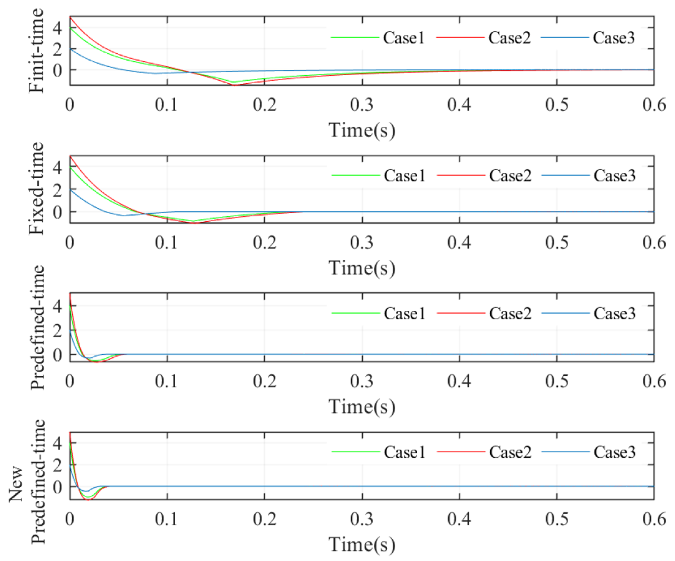
5.1. Simulation Analysis

The parameters of the permanent magnet synchronous motor used in the simulation and experiment of this paper are shown in

Table 1. Experimental platform parameters.

Items	Value	Parameters	Value
Rated speed	3000 RPM	$k_1$	0.8
Rated power	64 W	$k_2$	0.3
Rated current	4 A	$k_3$	0.1
Rated toque	0.2 N·m	$g_1$	−11,347
Pole pairs $p_n$	4	$g_2$	−37,250
Stator resistance $R_s$	$0.89\pm 10\%\mathrm{\Omega }$	$g_3$	−1389
Stator inductance $L_s$	0.62 ± 20% mH	${\lambda }_1$	0.3
Flux linkage ${\psi }_f$	0.00835 Wb	${\lambda }_2$	$1.2\times {10}^{-3}$
Rotational inertia $\mathit{J}$	0.028 $\mathrm{kg}·{\mathrm{m}}^2$	${\lambda }_3$	$1.7\times {10}^{-5}$

. In order to demonstrate the superiority of the observation system proposed in this paper more intuitively, the parameters of the current loop controller are set to be the same and the simulation time of the system is fixed to be 3 s, and the fixed step size is set to be 1 μs.

From the above analysis, it can be seen that the ability to accurately obtain the real-time rotational speed of the motor will greatly affect the mechanical parameter observer accuracy. The analysis of controller performance can be divided into the following steps: Firstly, the rotor information obtained by the sensorless algorithm is averaged and used as the control input. Second, the four controller models are simulated with three different gain conditions, respectively. Finally, the sliding mode surface waveforms and output waveforms of each controller are compared and analyzed.

As can be seen in Figure 4, the output waveforms of each control are significantly different when three parameter schemes are used for each of the four controllers. The finite time control scheme has the slowest convergence of the system error, which is about 0.45 s; followed by the fixed time control scheme, which is about 0.23 s; the traditional predefined control scheme has a shorter convergence time of the system error, which is only about 0.06 s; and the new predefined-time controller designed in this paper has the strongest convergence, which is about 0.04 s. It can, therefore, be concluded that the new predefined time sliding mode proposed in this paper controller has the shortest convergence time of the error system.

Analyzing Figure 5 shows that when the controllers are the same, a large difference in the gain parameters also affects the convergence speed of the sliding mode surface. When the gain parameters of the controllers are the same, the shortest convergence time of the sliding mode surface is for the new predefined sliding mode controller and the longest convergence time is for the finite time sliding mode controller. Therefore, analyzing Figure 4 and Figure 5, it can be concluded that the new predefined sliding mode controller has the shortest convergence time (sliding mode surface convergence time + error system convergence time).

In order to verify the observation performance of the IPESMO proposed in this paper, the values of each parameter of the motor are inputted into the model: $\mathit{J}$ = $0.028$ kg $·{\mathrm{m}}^2$, $\mathit{B}$ = 0.0017 N·m·s/rad, and $T_L$ = 0.2 N·m. In order to further analyze the response curves of the observation system when the load torque is varied, the load torque in the simulation model is set to be a step signal with an amplitude of 0.2, and the response to the output waveform of each observer is examined. Since the observation algorithm proposed in this paper can observe three different mechanical parameters simultaneously with one observer, and most of the current observation algorithms can only observe one mechanical parameter or have to use multiple algorithms to observe three different mechanical parameters, the comparison experiments in the simulation part of this paper adopt the algorithms that can observe two mechanical parameters at the same time: EMO and DESMO. The additional mechanical parameter $\mathit{B}$ will be used as a supplementary part in the final part. Parameter B will be shown as a supplementary section at the end.

Figure 6 shows the observed results of the system load torque. When the load torque steps from 0 to 0.2 at 1.5 s, the rotor speed decreases due to the increase in the load torque, but at this point, the self-regulating performance of the controller can readjust the motor speed to the desired speed. During this process, the estimated load torque waveform graph will change as the rotor speed changes, resulting in a non-zero speed differential. When the motor speed returns to a steady state, the estimated load torque will also stabilize. As can be seen from Figure 6, when the motor control system is the same, the ESO is susceptible to the influence of the external environment, and the robustness is weak, but after the observation system is stabilized, the accuracy of the observation is stable at about 0.2 N·m; DESMO has the characteristics of SMO and ESO at the same time, although it can make the observation system ensure the degree of accuracy required to reduce the impact of external parameter changes on the system, but its observation results show a larger amplitude of jitter vibration phenomenon. From Figure 6, it can be seen that the IPESMO proposed in this paper can guarantee to improve the robustness of the observing system while reducing the jitter phenomenon of the observation results, which can improve the response speed of the observing system and ensure the accuracy of the observing system at the same time.

Figure 7 shows the waveforms of load torque observed by DESMO, IPESMO and IPESMO with a robust activator. As can be seen in Figure 7, the coupling effect between the load torque and the moment of inertia will deteriorate the observation results when more than one mechanical parameter is observed at the same time, as evidenced by the negative values at the beginning of the observation results. Although the observations will still eventually stabilize at the target value, the response of the observer will be slower, with the coupling effect of the DESMO algorithm being particularly pronounced. The inclusion of a robust activator in the IPESMO observer model greatly reduces the impact of parameter coupling effects on the observer output results.

Since the coupling effect of the moment of inertia can be neglected, the difference between the estimates of the moment of inertia obtained by the algorithms is small, and more attention should be paid to the response speed and robustness of the algorithms at this time. Analyzing Figure 8, it can be seen that the DESMO observer needs 0.5 s to stabilize the observation value, while the IPESMO only needs 0.3 s to keep the observation system stable (the response speed is improved by about 40%). When the system is loaded suddenly, the DESMO needs 0.45 s to adjust the system, while the IPESMO only needs 0.25 s. Therefore, the convergence speed, response time and robustness of the IPESMO are all better than that of the DESMO.

Figure 9 shows the output value of the IPESMO observation system $\mathit{B}$. From Figure 9, it can be seen that the observation system reaches stability at 0.45 s, and the output result is about 0.05. When there is a sudden change in the operating conditions of the motor at 1.5 s, the observation system self-adjusts for about 0.25 s.

5.2. Experimental Verification

In order to test the observation performance of IPESMO in a real motor control system, an experimental platform as shown in Figure 10 was constructed. The control system is shown in Figure 2. In this study, the position sensorless vector control strategy is implemented by the STM32F407 microcontroller.

During the experiment, the motor was operated normally through the motor drive board and motor control board, and the experimental test waveform of the PC end upper computer was observed. At the same time, the load torque of the dynamometer connected to the motor was slowly increased, and the experimental waveform of the PC end upper computer was observed in real time. Figure 11 shows a detailed experimental logic diagram.

(1) Experiment 1: Estimation of friction coefficient. Before conducting the experiment, the viscous friction coefficient and Coulomb friction coefficient should be estimated first. The estimation method is as follows: Under the no-load condition of the motor, the motor is rotated forward/reverse at a uniform speed and calculated by equation $J{\dot{\omega }}_m=T_e-T_L-B{\omega }_m-Gsign\left({\omega }_m\right)$. In order to obtain a more accurate viscous friction coefficient and Coulomb friction coefficient, this paper will be based on different target speeds for several fitting experiments.

To evaluate the performance of our solution, it is necessary to know the viscosity and Coulomb friction coefficient of the experimental platform being built. Under no-load conditions, these two friction coefficients can be calculated based on the fitting results of the relationship between $T_e$ and ${\omega }_m$. To obtain accurate results, $T_e$ and ${\omega }_m$ corresponding to different speed commands were obtained for both forward and reverse rotation of the prototype motor. Based on the obtained results, we can use curve fitting method to determine these two friction coefficients, as shown in Figure 12: $T_e=1.23\times {10}^{-6}{\omega }_m^2+1.719\times {10}^{-3}{\omega }_m+1.368\times {10}^{-3}sign\left({\omega }_m\right)$, $T_e=-1.163\times {10}^{-6}{\omega }_m^2+1.682\times {10}^{-3}{\omega }_m-1.351\times {10}^{-3}sign\left({\omega }_m\right)$.

(2) Experiment 2: Comparison between the estimated speed and the actual speed of the position sensorless algorithm. It is known from the analysis of the algorithm that the change in the internal parameters of the motor will affect the performance of the speed control system and reduce the control accuracy, which, in turn, affects the rotor information obtained by the position sensorless observation algorithm. Therefore, this paper adopts the traditional sliding mode controller and the new predefined-time sliding mode controller to control the speed control system, respectively, and compares the actual speed obtained by the two algorithms with the estimated speed. In order to verify that the control algorithms have good control performance at several stages of motor operation, the motors are tested at 1000 rpm, 1500 rpm, 2000 rpm and 3000 rpm desired speeds, respectively.

As can be seen from Figure 13, when the control system adopts the new predefined time sliding mode controller, the actual speed of the motor will be stabilized within ±5 rpm of the desired speed, and at this time, the gap between the speed information observed by AGFSTA-SMO and the actual value is much smaller. At the same time, it can be clearly seen that the speed information obtained by the FSMC control algorithm is obviously reduced compared with that obtained by the SMC jitter amplitude. Because the performance of the controller has been improved, the resultant accuracy of the controller output is improved, the jitter amplitude is reduced, which, in turn, improves the accuracy of the AGFSTA-SMO observation, so that the results of the IPESMO estimation are more in line with the values of the actual mechanical parameters, which are eventually fed back into the control system to improve the control accuracy.

(3) Experiment 3: Comparison of estimation results with and without Coulomb friction torque compensation. When the desired speed of the motor is 1000 rpm and the load torque is zero, the Coulomb friction compensation comparison experiment is carried out. As can be seen from Figure 14 and Figure 15, before compensation $\widehat{J}\approx 0.0274$ (around 7% error), ${\widehat{T}}_L\approx 0.0089$ (around 16% error), $\widehat{B}\approx 0.0044$ (around 13% error), after compensation $\widehat{J}\approx 0.0278$ (around 2.5% error), ${\widehat{T}}_L\approx 0.0095$ (around 10.3% error), $\widehat{B}\approx 0.0048$ (around 12% error). Therefore, it can be concluded that when Coulomb friction torque compensation is used, the observed accuracy of each parameter will be further improved.

(4) Experiment 4: Different algorithms are used to observe the moment of inertia, load torque and viscous friction coefficient. From the waveforms of the observation results of each algorithm in Figure 16, it can be seen that when IPESMO is used to observe each mechanical parameter, it has the smallest error with respect to the reference value; the observation error obtained by DESMO is slightly larger than that of ESO, which is similar to that of the simulation results, and the observation results have obvious jitter near the desired value because DESMO still has the drawbacks of SMO. From Figure 17, it can be seen that the observation error of each parameter obtained by IPESMO is the smallest, and the observation error of each parameter obtained by DESMO is the largest.

(5) Experiment 5: The effect of different observer gains on parameter estimation. It is known from the analysis of the observer principle that different observer gains will affect the identification accuracy of the observer, the convergence speed of the slip mode surface and the jitter amplitude of the observation results. In order to further study the influence weight of the gain parameters, the IPESMO observer gain is set to 0.1, 0.3 and 0.8, respectively, and the output results of the observer are analyzed.

Analyzing Figure 18, it can be seen that when the observer gain is 0.8, the output results of the observer have the slowest convergence speed and lower jitter amplitude. When the observer gain is 0.3, the convergence speed of the observer is significantly improved compared to the former, but the jitter amplitude of the output results increases. Although the average value of the observation results remains unchanged, the jitter of the observation results will inevitably affect the identification of other mechanical parameters. When the gain of the observer is 0.1, the convergence speed of each parameter observer reaches the fastest, and the jitter is kept small.

(6) Experiment 6: Comparison of the estimation results of each algorithm when the load torque is different. In order to verify the adaptability of the load observer, the load torque is increased to 0.1 N·m and 0.2 N·m, and the output results are observed. When the motor is connected to the dynamometer, because the coupling itself has a certain mass, and when the motor drives the dynamometer to rotate, it is bound to be subjected to a certain amount of resistance; so, when the load torque output from the dynamometer is 0, the actual load torque should be slightly greater than 0, and the load torque at this time is about 0.01 N.m. When the load torque is set to 0.1 N.m and 0.2 N.m, the load torque influence brought by the equipment itself is ignored.

As can be seen from Figure 19, when the motor load torque is set to 0.1 N·m and 0.2 N·m, respectively, the liability torque observed by the IPESMO algorithm is the closest to the actual torque, followed by the observation obtained by the ESMO algorithm, and the observation obtained by the DESMO algorithm has the largest error with the actual value, which is probably due to the coupling error effect and the poor convergence of the observer.

6. Conclusions

In this paper, a novel cross-interconnected dilated sliding mode observer is proposed, which can accurately observe the parameters of the moment of inertia, load torque and the viscous friction coefficient of the motor when the motor is running. A novel predefined time sliding mode controller is designed which can improve the observation accuracy and immunity to disturbances of the control system, and both are combined to design a position sensorless control system for a permanent magnet synchronous motor. Three simultaneous observers were built using the ESO principle to enable the online simultaneous identification of three mechanical parameters. In this paper, the design process of the observer not only increases the amount of compensation for the Coulomb friction torque, but also separately designs the gain parameters for different mechanical parameter observers, and also incorporates a robust activator in the process of parameter design. Thus, the observed values of each mechanical parameter are more accurate, and the results fluctuate less during the sudden change in the operating conditions of the motor. In the design of the predefined time sliding mode controller, the effects of different motor models on the controller are fully considered, and the controller is improved from the controller’s point of view by means of designing a new sliding mode surface and an incremental legacy function. Finally, the observation system and the control system are combined, which proves the convergence and stability of the whole operation system. Simulation and experimental results show that the control strategy adopted in this paper has the advantages of fast convergence, high accuracy and robustness. Future research will focus on reducing the number of gain parameters and improving the self-adjustment ability of each parameter, reducing the difficulty of tuning the parameters, and transplantation of the observer algorithm.

References

1. Zuo, Y.; Lai, C.; Iyer, K.L.V. A review of sliding mode observer based sensorless control methods for PMSM drive. IEEE Trans. Power Electron. 2023, 38, 11352–11367. [Google Scholar] [CrossRef]
2. Ding, S.; Hou, Q.; Wang, H. Disturbance-observer-based second-order sliding mode controller for speed control of PMSM drives. IEEE Trans. Energy Convers. 2022, 38, 100–110. [Google Scholar] [CrossRef]
3. Xiao, F.; Chen, Z.; Chen, Y.; Liu, H. A finite control set model predictive direct speed controller for PMSM application with improved parameter robustness. Int. J. Electr. Power Energy Syst. 2022, 143, 108509. [Google Scholar] [CrossRef]
4. Hou, Q.; Ding, S. Finite-time extended state observer-based super-twisting sliding mode controller for PMSM drives with inertia identification. IEEE Trans. Transp. Electrif. 2021, 8, 1918–1929. [Google Scholar] [CrossRef]
5. Liu, Y.C.; Laghrouche, S.; Depernet, D.; Djerdir, A.; Cirrincione, M. Disturbance-observer-based complementary sliding-mode speed control for PMSM drives: A super-twisting sliding-mode observer-based approach. IEEE J. Emerg. Sel. Top. Power Electron. 2020, 9, 5416–5428. [Google Scholar] [CrossRef]
6. Li, S.; Xu, Y.; Zhang, W.; Zou, J. Robust deadbeat predictive direct speed control for PMSM with dual second-order sliding-mode disturbance observers and sensitivity analysis. IEEE Trans. Power Electron. 2023, 38, 8310–8326. [Google Scholar] [CrossRef]
7. Yildiz, R.; Demir, R.; Barut, M. Online estimations for electrical and mechanical parameters of the induction motor by extended Kalman filter. Trans. Inst. Meas. Control 2023, 45, 2725–2738. [Google Scholar] [CrossRef]
8. Miloud, I.; Cauet, S.; Etien, E.; Salameh, J.P.; Ungerer, A. Real-Time Speed Estimation for an Induction Motor: An Automated Tuning of an Extended Kalman Filter Using Voltage–Current Sensors. Sensors 2024, 24, 1744. [Google Scholar] [CrossRef] [PubMed]
9. İnan, R.; Aksoy, B.; Salman, O.K.M. Estimation performance of the novel hybrid estimator based on machine learning and extended Kalman filter proposed for speed-sensorless direct torque control of brushless direct current motor. Eng. Appl. Artif. Intell. 2023, 126, 107083. [Google Scholar] [CrossRef]
10. Yang, C.; Song, B.; Xie, Y.; Zheng, S.; Tang, X. Adaptive identification of nonlinear friction and load torque for PMSM drives via a parallel-observer-based network with model compensation. IEEE Trans. Power Electron. 2023, 38, 5875–5897. [Google Scholar] [CrossRef]
11. Liu, Y.C.; Laghrouche, S.; Depernet, D.; N’Diaye, A.; Djerdir, A.; Cirrincione, M. Super-twisting sliding-mode observer-based model reference adaptive speed control for PMSM drives. J. Frankl. Inst. 2023, 360, 985–1004. [Google Scholar] [CrossRef]
12. Zhu, H.; Zhu, J.; Jiang, D.; Mao, B.; Liu, Y. Displacement Self-sensing Control of Outer Rotor Coreless Bearingless Permanent Magnet Synchronous Motor Based on Least Square Support Vector Machine Optimised by IMFO. IEEE Trans. Power Electron. 2024, 40, 716–726. [Google Scholar] [CrossRef]
13. Zhu, H.; Shi, Y. Displacement self-sensing control of permanent magnet assisted bearingless synchronous reluctance motor based on least square support vector machine optimized by improved NSGA-II. IEEE Trans. Ind. Electron. 2023, 71, 1201–1211. [Google Scholar] [CrossRef]
14. Nachtsheim, M.; Ernst, J.; Endisch, C.; Kennel, R. Performance of Recursive Least Squares Algorithm Configurations for Online Parameter Identification of Induction Machines in an Automotive Environment. IEEE Trans. Transp. Electrif. 2023, 9, 4236–4254. [Google Scholar] [CrossRef]
15. Yang, C.; Song, B.; Xie, Y.; Lu, S.; Tang, X. Speed-controller-independent mechanical parameter identification in SPMSM drive achieved via signal injection. IEEE Trans. Ind. Electron. 2022, 70, 1282–1297. [Google Scholar] [CrossRef]
16. Fazdi, M.F.; Hsueh, P.W. Parameters identification of a permanent magnet dc motor: A review. Electronics 2023, 12, 2559. [Google Scholar] [CrossRef]
17. Feng, Y.; Yu, X.; Han, F. High-order terminal sliding-mode observer for parameter estimation of a permanent-magnet synchronous motor. IEEE Trans. Ind. Electron. 2012, 60, 4272–4280. [Google Scholar] [CrossRef]
18. Zhang, X.; Li, Z. Sliding-mode observer-based mechanical parameter estimation for permanent magnet synchronous motor. IEEE Trans. Power Electron. 2015, 31, 5732–5745. [Google Scholar] [CrossRef]
19. Boileau, T.; Leboeuf, N.; Nahid-Mobarakeh, B.; Meibody-Tabar, F. Online identification of PMSM parameters: Parameter identifiability and estimator comparative study. IEEE Trans. Ind. Appl. 2011, 47, 1944–1957. [Google Scholar] [CrossRef]
20. Garrido, R.; Concha, A. Inertia and friction estimation of a velocity-controlled servo using position measurements. IEEE Trans. Ind. Electron. 2013, 61, 4759–4770. [Google Scholar] [CrossRef]
21. Lozada-Castillo, N.; Chairez, I.; Luviano-Juarez, A.; Escobar, J. Parameter identification of a permanent magnet synchronous motor. In Proceedings of the 53rd IEEE Conference on Decision and Control, Los Angeles, CA, USA, 15–17 December 2014; IEEE: Piscataway, NJ, USA, 2014; pp. 1005–1010. [Google Scholar]
22. Xu, B.; Zhang, L.; Ji, W. Improved non-singular fast terminal sliding mode control with disturbance observer for PMSM drives. IEEE Trans. Transp. Electrif. 2021, 7, 2753–2762. [Google Scholar] [CrossRef]
23. Xu, Y.; Li, S.; Zou, J. Integral sliding mode control based deadbeat predictive current control for PMSM drives with disturbance rejection. IEEE Trans. Power Electron. 2021, 37, 2845–2856. [Google Scholar] [CrossRef]
24. Belkhier, Y.; Oubelaid, A. Passivity-based Control of PMSM Servo System with Load Torque Adaptation: Theoretical and Experimental Validation. IEEE Trans. Transp. Electrif. 2024. [Google Scholar] [CrossRef]
25. Yi, P.; Wang, X.; Chen, D.; Sun, Z. PMSM current harmonics control technique based on speed adaptive robust control. IEEE Trans. Transp. Electrif. 2021, 8, 1794–1806. [Google Scholar] [CrossRef]
26. Zheng, Y.; Zhao, H.; Zhen, S.; He, C. Designing robust control for permanent magnet synchronous motor: Fuzzy based and multivariable optimization approach. IEEE Access 2021, 9, 39138–39153. [Google Scholar] [CrossRef]
27. Cao, Z.; Mao, J.; Zhang, C.; Cui, C.; Yang, J. Safety-Critical Generalized Predictive Control for Speed Regulation of PMSM Drives Based on Dynamic Robust Control Barrier Function. IEEE Trans. Ind. Electron. 2024. [Google Scholar] [CrossRef]
28. Bouguenna, I.F.; Tahour, A.; Kennel, R.; Abdelrahem, M. Multiple-vector model predictive control with fuzzy logic for PMSM electric drive systems. Energies 2021, 14, 1727. [Google Scholar] [CrossRef]
29. Kivanc, O.C.; Ozturk, S.B. Sensorless PMSM drive based on stator feedforward voltage estimation improved with MRAS multiparameter estimation. IEEE/ASME Trans. Mechatronics 2018, 23, 1326–1337. [Google Scholar] [CrossRef]
30. Elmas, C.; Ustun, O.; Sayan, H.H. A neuro-fuzzy controller for speed control of a permanent magnet synchronous motor drive. Expert Syst. Appl. 2008, 34, 657–664. [Google Scholar] [CrossRef]
31. Nguyen, A.T.; Rafaq, M.S.; Choi, H.H.; Jung, J.W. A model reference adaptive control based speed controller for a surface-mounted permanent magnet synchronous motor drive. IEEE Trans. Ind. Electron. 2018, 65, 9399–9409. [Google Scholar] [CrossRef]
32. Hashjin, S.A.; Pang, S.; Miliani, E.H.; Ait-Abderrahim, K.; Nahid-Mobarakeh, B. Data-driven model-free adaptive current control of a wound rotor synchronous machine drive system. IEEE Trans. Transp. Electrif. 2020, 6, 1146–1156. [Google Scholar] [CrossRef]
33. Qi, L.; Shi, H. Adaptive position tracking control of permanent magnet synchronous motor based on RBF fast terminal sliding mode control. Neurocomputing 2013, 115, 23–30. [Google Scholar] [CrossRef]
34. Zhang, B.; Pi, Y.; Luo, Y. Fractional order sliding-mode control based on parameters auto-tuning for velocity control of permanent magnet synchronous motor. ISA Trans. 2012, 51, 649–656. [Google Scholar] [CrossRef] [PubMed]
35. Lu, E.; Li, W.; Wang, S.; Zhang, W.; Luo, C. Disturbance rejection control for PMSM using integral sliding mode based composite nonlinear feedback control with load observer. ISA Trans. 2021, 116, 203–217. [Google Scholar] [CrossRef] [PubMed]
36. Hu, Y.; Liu, K.; Hua, W.; Hu, M. First-order model based inductance identification with least square method for high-speed sensorless control of permanent magnet synchronous machines. IEEE Trans. Power Electron. 2023, 38, 8719–8729. [Google Scholar] [CrossRef]
37. Liu, K.; Zhu, Z. Fast Determination of Moment of Inertia of Permanent Magnet Synchronous Machine Drives for Design of Speed Loop Regulator. IEEE Trans. Control Syst. Technol. 2017, 25, 1816–1824. [Google Scholar] [CrossRef]
38. Wang, S.; Wan, S. Full digital deadbeat speed control for permanent magnet synchronous motor with load compensation. IET Power Electron. 2013, 6, 634–641. [Google Scholar] [CrossRef]
Figure 1. Voltage equivalent circuit diagram.
Actuators 13 00525 g001
Figure 2. Block diagram of permanent magnet synchronous motor control system.
Actuators 13 00525 g002
Figure 3. Block diagram of the observer principle.
Actuators 13 00525 g003
Figure 4. Convergence of the error system for different control schemes.
Actuators 13 00525 g004
Figure 5. Curves at convergence of sliding mode surface for different control schemes.
Actuators 13 00525 g005
Figure 6. Single-state observer load torque observation results.
Actuators 13 00525 g006
Figure 7. Multi- state observer load torque observation results.
Actuators 13 00525 g007
Figure 8. Multi-state observer rotational inertia observation results.
Actuators 13 00525 g008
Figure 9. Observations of B when using the IPESMO algorithm.
Actuators 13 00525 g009
Figure 10. Experimental control platform.
Actuators 13 00525 g010
Figure 11. Experimental logic diagram.
Actuators 13 00525 g011
Figure 12. Fitting of the friction coefficients on the test bench. (A) Motor reversal. (B) Motor forward.
Actuators 13 00525 g012
Figure 13. Actual and estimated motor speeds obtained using the SMC and NFTSMC algorithms, respectively, when the desired speeds are different. (A) 1000 rpm. (B) 1500 rpm. (C) 2000 rpm. (D) 3000 rpm.
Actuators 13 00525 g013
Figure 14. Comparison of estimation results with and without Coulomb friction torque compensation. (A) With compensation J ^ . (B) With compensation T ^ L . (C) With compensation B ^ . (D) Without compensation J ^ . (E) Without compensation T ^ L . (F) Without compensation B ^ .
Actuators 13 00525 g014
Figure 15. Comparison of errors with and without Cullen friction torque compensation.
Actuators 13 00525 g015
Figure 16. (A) IPESMO. (B) DESMO. (C) ESO.
Actuators 13 00525 g016
Figure 17. Comparison of the errors in the observations of the three algorithms.
Actuators 13 00525 g017
Figure 18. Comparison of observed values of each mechanical parameter at different times of gain. (A) Observation value of J. (B) Observation value of T L . (C) Observation value of B.
Actuators 13 00525 g018
Figure 19. Multi-load multi-algorithm comparison experiments. (A) IPESMO −0.1 N·m. (B) ESMO −0.1 N·m. (C) DESMO −0.1 N·m. (D) IPESMO −0.2 N·m. (E) ESMO −0.2 N·m. (F) DESMO −0.2 N·m.
Actuators 13 00525 g019