Abstract
To address the multi-peak characteristics of the P-U output characteristic curve when the photovoltaic array is partially shaded, a Maximum Power Point Tracking (MPPT) method combining Harris Hawk optimization, and a variable step conductance increment method is proposed in this article. Although the Harris Hawk Optimization algorithm has advantages in optimizing multi-modal P-U curves, when the lighting conditions suddenly change, the output characteristic curve will undergo drastic changes, causing the algorithm to oscillate repeatedly at the maximum power point. Moreover, due to its inherent limitations, the Harris Hawk algorithm has a low convergence accuracy, slow tracking speed, and is prone to getting trapped in a local optimum. In order to compensate for the shortcomings of the Harris Hawk Optimization algorithm, the variable step conductance increment method is switched for local exploration to improve the algorithm’s ability to escape from the local optimal solution and reduce power oscillation. Finally, the MPPT control of the proposed strategy was simulated and verified on the MATLAB/Simulink simulation (2021) platform. In the MPPT test experiment, the proposed composite algorithm was applied to simulate and verify uneven irradiance conditions.
1. Introduction
Solar photovoltaic technology, which has been in use since the early 1970s, has undergone a long process of development. Initially, the application of this technology was relatively limited, but in recent years, the solar photovoltaic industry has experienced rapid growth and has become one of the most critical renewable energy technologies in the world [1]. Solar power generation is susceptible to weather conditions, such as overcast and snowy weather conditions that can partially obstruct the solar panels, preventing them from receiving even lighting. These conditions will lead to a position where the photovoltaic cell operating point may not always be at the maximum power, and there is a power multi-peak phenomenon, which will affect the power generation efficiency of photovoltaic cells [2,3]. In order to use solar energy efficiently, some scholars have focused their research on Maximum Power Point Tracking (MPPT).
Traditional Maximum Power Point Tracking methods, such as the constant voltage method, the increment conductance method (INC), and the perturbation and observation method (P&O), are suitable for single-peak optimization under uniform illumination [4]. The increment conductance method (INC) and the perturbation and observation method (P&O) were improved with a variable step size. According to the relationship between the actual photovoltaic working point position and the maximum power point position, the step size is changed in real time to improve the tracking effect, including improving the response speed and reducing the system oscillation [5,6]. However, when light irradiation becomes uneven due to the external environment, the P-U curve of the photovoltaic array exhibits multi-peak characteristics [7], and traditional control methods face the problem of failure.
In view of the above problems, domestic and foreign scholars have studied and proposed the application of intelligent algorithms. The literature [8] introduces a control strategy that combines a prediction model and a perturbation observation method, which can quickly and accurately track MPPT in a constantly changing environment. However, this method requires an understanding of the mathematical model of the system, which is difficult to implement. In reference [9], an improved particle swarm optimization (IPSO) algorithm was proposed to improve the tracking speed of the system in view of the situation of the traditional particle swarm optimization (PSO) algorithm in the local shadow environment. Although the maximum power tracking speed has been improved, there are still fluctuations in the output power. The literature [10] proposes an immune firefly algorithm that uses a vaccine library to accelerate the search process and improves the accuracy and stability of the algorithm through immune enhancement and elimination of inefficient individuals. However, this algorithm has a slow convergence speed, is easy to fall into local optimum, and has an early convergence, which limits its effectiveness and efficiency. The literature [11,12] introduced a particle swarm optimization algorithm and ANN neural network using adaptive variation strategy to design a MPPT controller, aiming to improve the accuracy of photovoltaic MPPT, but the control effect of the neural network may be limited by weight adjustment, and the PSO algorithm has a slow convergence rate. The literature [13] discusses a composite algorithm combining PSO, a genetic algorithm, and a fuzzy control. By combining the advantages of the first two algorithms and introducing a fuzzy control, the output fluctuation and power loss when the maximum power point (MPP) is reached can be reduced. However, the control model of this composite algorithm is complex, the computation is large, and the optimization speed is not significantly improved. In the literature [14], the improved gray Wolf optimization algorithm was adopted for maximum power point tracking. However, while the tracking speed was effectively improved, there was a power oscillation problem in the algorithm optimization process, resulting in a certain power loss. In [15], Harris Hawk Optimization (HHO) was proposed by imitating Harris Hawk, which has a strong global search ability and does not require complicated parameter tuning. However, the Harris Hawk algorithm has a low convergence accuracy, a slow tracking speed, and is prone to getting trapped in a local optimum. The literature [16,17] comprehensively compares all kinds of algorithms, and the composite algorithm is more balanced in performance and complexity.
Aiming at the shortcomings of the above algorithms, this paper proposes a MPPT strategy based on the Harris Hawk optimization (HHO) algorithm to solve the problem where the traditional maximum power easily falls into a local optimal and is difficult to balance tracking accuracy and speed. The rest of this article is organized as follows. In Section 2, the working principle of photovoltaic cells is introduced, its mathematical modeling is carried out, and the working characteristics of photovoltaic cells are simulated and analyzed in MATLAB/Simulink for different conditions under different lighting conditions. The P-U curves of its output are analyzed for uniform and non-uniform lighting conditions. Then, the Harris Hawk optimization (HHO) algorithm is introduced in Section 3. Aiming at the problem where the traditional MPPT algorithm easily falls into a local optimal in the case of a multi-peak value, which leads to the decrease of system efficiency. Section 4 introduces a matching algorithm based on Harris Hawk optimization (HHO) and the variable step length conductance increment method (INC). The experiment results are presented in Section 5 to prove the accuracy of the analyses and the effectiveness of the proposed MPPT algorithm. Finally, the conclusions are drawn in Section 6.
2. Principle and Characteristic Analysis of Photovoltaic Cell
The photovoltaic power generation system mainly consists of three parts: photovoltaic array, MPPT controller, and DC–DC conversion unit. Because isolation is very important in practical applications, according to reference [18], the authors of this paper adopted an isolation type DC–DC converter. The task of the MPPT controller is to adjust the working state of the photovoltaic array in real time to ensure that the maximum output power can be captured under any given environmental conditions. Photovoltaic cells provide output voltage for the entire system. As the energy source of photovoltaic power generation systems, the higher its conversion rate, the more energy the system can get, and the higher the system power generation efficiency. The position of the photovoltaic cell operating point will change due to changes in the external environment, which may mean the maximum power point changes. Only by making the photovoltaic work at its MPP at all times can the high utilization rate of solar energy be maintained. Therefore, to study the efficiency of a photovoltaic power generation system, we must study the mathematical model and output characteristics of photovoltaic cells.
2.1. Mathematical Model of Photovoltaic Cell
The equivalent circuit of the photovoltaic cell is shown in Figure 1, and are the resistances generated by no ideal effects in photovoltaic cells, and is photocurrent.
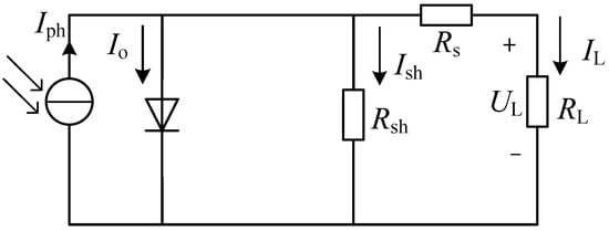
Figure 1.
Photovoltaic cell equivalent model.
According to the equivalent circuit diagram of the photovoltaic cell, the output current expression can be obtained as:
where and are the output voltage and current of a single photovoltaic cell, respectively; n is the diode index; K is the Boltzmann constant; q is the unit charge; is the external temperature.
Due to the small value of and the large value of , the last term in expression (1) can be ignored. For ease of application, Equation (1) can be simplified as follows:
where represents short-circuit current; represents open circuit voltage.
When the photovoltaic cell outputs its maximum power, , the expressions for and are as follows:
2.2. Multi-Peak Characteristics of Photovoltaic Arrays
The local shadows generated by obstructions in photovoltaic arrays can cause the P-U curve of the photovoltaic array to exhibit multi-peak characteristics. To further research multi-peak optimization control methods to improve photovoltaic power generation efficiency, a photovoltaic array model in MATLAB/Simulink was built, considering the occlusion situation of the photovoltaic array the situation is shown in Table 1. The open circuit voltage of the photovoltaic cell is 35 V, the short circuit current is 7.5 A, and the MPP voltage, and currents are 28 V and 7 A, respectively.

Table 1.
Irradiance of each component of photovoltaic array.
The P-U characteristic curves of the photovoltaic array are shown in Figure 2. The gray curve is the equivalent resistance load characteristic curve corresponding to MPP under standard conditions. From Figure 2, the four lines in the graph represent P-U curves under four different lighting conditions, and each point represents an extreme point on the corresponding curve, it can be seen that the photovoltaic array will have multiple extreme points in the case of local occlusion. The classical perturbation based MPPT algorithm may mistakenly identify one of the multiple extreme points as the maximum point, resulting in a loss of success rate. Therefore, using the photovoltaic characteristic curve law to improve the MPPT algorithm with a stronger global search ability can effectively solve the problem.
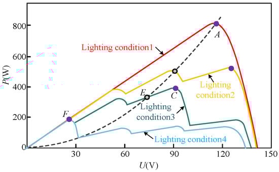
Figure 2.
Photovoltaic array output characteristic curve.
3. Proposed MPPT Technique Based on IHHO
According to the analysis of the output characteristics of photovoltaic cells in Section 2, it is concluded that the output power of solar cells is greatly affected by light. Therefore, only by ensuring that the output power remains stable at the maximum point under any lighting conditions can the system efficiency be optimized. In response to multiple local power peaks caused by local shading, this chapter proposes an improved Harris Hawk algorithm.
In the Harris Hawk Optimization algorithm, each Harris Hawk represents a potential solution, and the goal pursued in each iteration represents the global optimal solution. The hunting stage of this population is mainly divided into three stages: the research stage, the transition stage between search and development, and the development stage.
In the initial stage, the algorithm performs a global search, with Harris Hawks randomly distributed in the solution space, waiting for opportunities within the search range and searching for prey. During the search process, they will constantly change their positions based on two different strategies to approach the target. The specific mathematical expression is:
where t is the current iteration count; is the position of individual i after the t-th iteration; represents randomly selecting individual positions after t iterations; , and q represents a constant between 0 and 1; and represent the upper and lower limits of the search space; represents the average position of the population after t iterations, its expression as follows:
where N is the population size.
The HHO algorithm can flexibly switch between exploration and development stages and can adjust its development strategy based on the remaining energy of prey. As the prey’s energy gradually depletes, their escape behavior will affect the hunting methods of the eagle flock, causing them to dynamically switch between different search and development behaviors based on the prey’s energy level . When , enter the global search phase; When , enter the local development phase. The formula for escape energy is:
where represents the initial energy state of the prey, which is a random number of . As the number of iterations increases, the escape energy decreases.
When the escape energy , HHO enters the development phase and begins to implement local search. Based on the hunting characteristics of Harris eagles, four different strategies were developed to perform local searches and rearrange their positions, taking into account variables such as the size of E and whether the prey escaped or not. R represents the probability of escape. When , the prey successfully escapes; , Harris Eagle will conduct a hunt. The escape energy E is used to determine the strategy, and for the judgment of the encirclement strategy: when , a soft encirclement strategy is adopted; When , adopt a hard siege.
Soft Siege: When and , the prey has energy to escape but ultimately fails, and the Harris Eagle adopts a soft encirclement strategy. At this point, Harris Eagle will update its position according to Equation (7):
where represents the next update position of Harris Hawk, represents the distance between the current prey and Harris Hawk, and represents the jumping intensity of the prey, which is a random number within that varies with iteration.
Hard Siege: When and , the prey has no energy to escape, and the Harris Hawk does not need to wait for a direct attack. At this point, use the following equation to update the current position:
Accumulated speed diving soft siege: When and , the escape energy is sufficient, and the prey successfully escapes. Harris hawks still use soft siege before attacking their prey. In the HHO algorithm, the Levy flight module is introduced to simulate the escape and jumping behavior of prey, corresponding to a new position update strategy. By introducing it, the convergence speed and optimization ability of the system are enhanced. During Levy’s flight, the Harris Hawk will follow a specific position update strategy to ensure that the search direction and range meet actual needs:
where is the dimension of the current problem, S is a random row vector, LF is the Levy flight function, which is calculated using Equation (12):
Accumulated speed diving hard siege: When and , if the prey cannot escape, the Harris Hawk will adopt a hard siege strategy to capture the prey. Update the location according to the following strategy:
According to the above steps, the flowchart of HHO algorithm is as Figure 3:
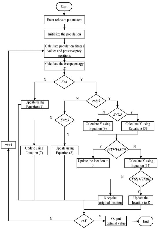
Figure 3.
HHO algorithm flow.
4. Proposed Improved MPPT Algorithm Is Based on HHO and INC
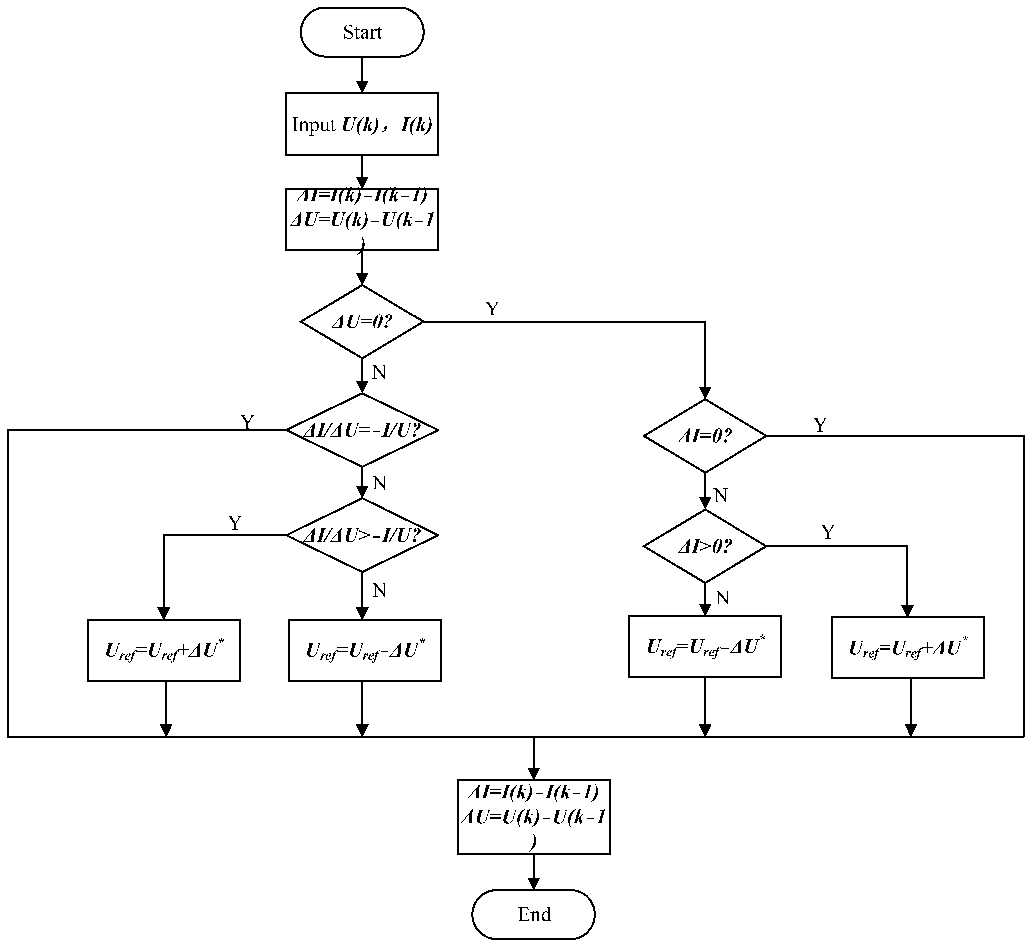
The fixed step conductance increment method can quickly track the maximum power point, and the tracked position is also very accurate. However, due to the fixed step size, this method has contradictions in terms of accuracy and speed. The variable step size conductance increment method adjusts the step size by the difference between the operating point and the maximum power point position, improving the problem of oscillation at the maximum power point and achieving better steady-state performance.
The step size of INC varies from large to small according to the rule of infinitely approaching MPP based on its distance from MPP. Until it decreases to zero, it indicates that the maximum power point has been reached. The problem of oscillation in the fixed step INC algorithm at the maximum power point has been solved by using a variable step tracking method.
When the external environment is in a steady state, the derivative of the output power of the battery can be expressed as:
From the above analysis, the system is at its maximum power point when . In INC, the relationship between the voltage and current of the system and its conductivity needs to satisfy the following conditions:
When , the maximum power point is located to the right of that point; When , this point is the maximum power point; When , the maximum power point is on the left side of that point. The basic principle of the incremental conductance method is shown in Figure 4.
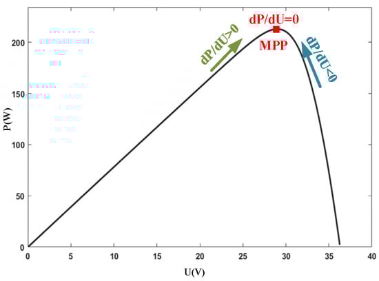
Figure 4.
Schematic diagram of variation on characteristic curve.
The incremental conductance method has demonstrated significant stability in the maximum power point tracking control of photovoltaic power generation. This method can accurately adapt to external environmental conditions, such as changes in irradiance, and achieve effective response to environmental changes. Its tracking effect is not affected by the performance characteristics of the photovoltaic module or the specific parameters of the battery, ensuring robust tracking of the optimal power point by the system. The flowchart of the incremental conductance method is shown in Figure 5.

Figure 5.
INC algorithm flowchart.
Although the Harris Hawk algorithm has advantages in optimizing multi-modal P-U curves, when the lighting conditions suddenly change, the output characteristic curve will undergo drastic changes, causing the algorithm to oscillate repeatedly at the maximum power point. Moreover, the Harris Hawk algorithm is prone to getting stuck in local optima in the later stages of iteration due to its inherent characteristics. Therefore, combining the HHO algorithm with the variable step size INC algorithm, and then transitioning to the variable step size INC in the later stage of HHO algorithm optimization, can improve the algorithm’s ability to jump out of local optima and reduce power oscillations, thereby increasing its stability. When the HHO algorithm reaches the number of iterations, terminate the algorithm to output the optimal solution, satisfy the following Equation (18), and switch to the variable step INC algorithm.
where and represent the power of the first and second cycles, respectively; is the maximum allowable power variation.
Based on the above analysis, when designing a photovoltaic power generation system, isolation requirements are important. According to reference [18], this design employs an isolation DC–DC converter. The system structure diagram of the isolated photovoltaic maximum power point tracking mode is shown in Figure 6.
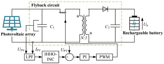
Figure 6.
Structure of the isolated PV system.
5. Simulation Analysis
In order to verify whether the proposed algorithm can achieve the task of tracking the maximum power point of photovoltaic power generation while balancing tracking accuracy and speed, this section uses a MATLAB/Simulink (2021) simulation platform to simulate MPPT control based on a IHHO-INC composite algorithm.
The simulation model diagram is shown in Figure 7, mainly composed of four modules: a photovoltaic array model, a DC–DC converter, a PWM pulse signal model, and a MPPT controller model. Among them, the battery is used instead of the load.
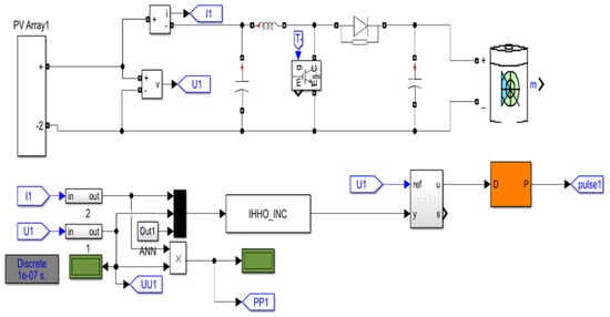
Figure 7.
Control simulation model diagram.
This article takes a 12 × 1 photovoltaic array as an example to build an MPPT control model. The parameters of the photovoltaic cells under standard test conditions are shown in Table 2.
Table 2.
Battery parameters under standard testing conditions.
Firstly, the traditional MPPT control algorithm was simulated and analyzed under the standard conditions of S = 1000 W/m2 and T = 25 °C. The simulation results obtained for a single photovoltaic array are shown in Figure 8. The I curves under variable step conductance increment method and incremental conductance method (INC) are shown in Figure 8a, Figure 8b shows the U curves under the two methods, and Figure 8c presents the P curves under the two methods.
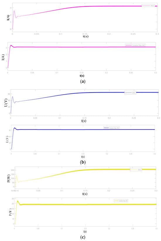
Figure 8.
Output I, U, P curves under variable step conductance increment method and incremental conductance method: (a) The I curves of the two methods (b) The U curves of the two methods (c) The P curves of the two methods.
The INC algorithm finds the maximum power point at 0.15 s, and the variable step conductance increment method finds the maximum power point at 0.017 s. It can be concluded that the variable step conductance method has a better steady-state performance and can find the maximum power point in a shorter time.
In order to verify the superiority of the MPPT control strategy applied in this paper, the experimental results of commonly used and effective particle swarm optimization algorithm, the Harris Hawk algorithm, and the IHHO-INC composite algorithm proposed in this paper were compared and analyzed at an ambient temperature of T = 25 °C. Simulation comparison analysis was conducted under uniform and non-uniform lighting conditions. The parameter settings are shown in the following Table 3:
Table 3.
Photovoltaic array illumination intensity setting.
Three algorithms: PSO, IPSO, HHO, IHHO-INC, output voltage, and output power curves under uniform irradiation are shown in Figure 9, and the output voltage and power curves under non-uniform irradiation are shown in Figure 10.

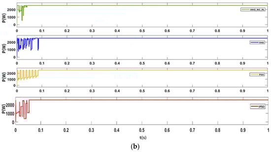
Figure 9.
Comparison curves of U and P output by three algorithms under uniform lighting conditions: (a) four algorithms output U-curves under uniform lighting conditions; (b) four algorithms output P-curves under uniform lighting conditions.
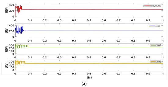
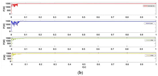
Figure 10.
Four algorithms output U and P comparison curves under non-uniform lighting conditions: (a) Four algorithms output U-curves under non-uniform lighting conditions; (b) Four algorithms output P-curves under non-uniform lighting conditions.
From Figure 9a,b, it can be seen that the PSO, IPSO, HHO, and IHHO-INC algorithms can all track the maximum power point under uniform irradiance, with particle swarm optimization algorithm tracking the maximum power point of 2550 W in 0.09 s; IPSO tracking the maximum power point of 2552 W in 0.05 s; Harris Eagle algorithm tracking the maximum power point of 2555 W in 0.08 s; IHHO-INC composite algorithm tracking the maximum power point of 2557 W in 0.04 s, and the actual maximum power of the system in this environment was 2557.18 W, with a tracking accuracy of up to 99.97%.
From Figure 10, under non-uniform irradiance, the particle swarm algorithm tracked the maximum power point of 1467 W in 0.09 s, the improved particle swarm algorithm tracked the maximum power point of 1467 W in 0.06 s, the Harris Hawk algorithm tracked the maximum power point of 1469 W in 0.08 s, and the IHHO-INC composite algorithm tracked the maximum power point of 1470 W in 0.04 s.
Therefore, the improved Harris Hawk algorithm has a faster optimization speed and can accurately track the maximum power point under both uniform and non-uniform lighting conditions. And from the power waveform, it can be seen that its volatility is significantly reduced, indicating that the composite algorithm applied in this paper can reduce the power oscillation of the system and maintain the stable operation of the photovoltaic array.
Finally, the PSO, IPSO, HHO, and IHHO-NIC algorithms were simulated and validated in a non-uniform irradiance and irradiance mutation working environment. The irradiance of the photovoltaic array was set to 1000 W/m2 within 0–0.25 s, 600 W/m2 within 0.25–0.5 s, and 1000 W/m2 within 0.5–0.8 s to simulate dynamic shading conditions. The output current, voltage, and power curves are shown in Figure 11.
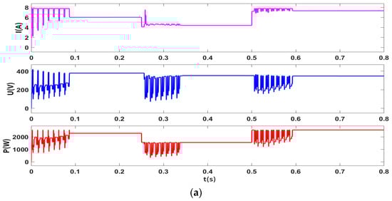
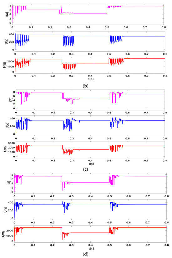
Figure 11.
Four algorithms output I, U, and P curves under non-uniform abrupt illumination: (a) Particle swarm optimization algorithm outputs I, U, and P curves under non-uniform abrupt illumination; (b) Improved particle swarm optimization algorithm outputs I, U, and P curves under non-uniform abrupt illumination; (c) HHO algorithm outputs I, U, and P curves under non-uniform abrupt illumination; (d) IHHO-INC composite algorithm outputs I, U, and P curves under non-uniform abrupt illumination.
As shown in Figure 11, under dynamic shading conditions, the particle swarm algorithm reduces power at 0.25 s, drops to 1551 W at 0.34 s, increases power at 0.5 s, and reaches 2550 W at 0.59 s; The improved particle swarm algorithm reduces power at 0.25 s, drops to 1551 W at 0.32 s, increases power at 0.5 s, and reaches 2555 W at 0.56 s; The Harris Hawk algorithm reduces power at 0.25 s, drops to 1548 W at 0.33 s, increases power at 0.5 s, and reaches 2555 W at 0.58 s; The power of the IHHO-INC composite algorithm reached 2557 W at MPP in 0.04 s, decreased due to a sudden change in irradiance at 0.25 s, and dropped to 1549 W at 0.29 s; At 0.5 s, the sudden change in irradiance caused a change in power, reaching 2556 W at 0.54 s; It can be seen that it takes 0.04 s to re-track to the maximum power point after each mutation, indicating that the composite algorithm completes optimization every 0.04 s.
In summary, at 0.25 s, the light intensity suddenly decreased to 600 W, compared with the simulation results, and the IHHO-INC algorithm proposed in this paper achieves the maximum power in the shortest time with higher accuracy. At 0.5 s, the light intensity suddenly increased again, and the IHHO-INC algorithm proposed in this paper still achieved the maximum power in the shortest time with higher accuracy. The experiment verifies that the IHHO-INC algorithm proposed in this paper has good stability when the light intensity suddenly changes.
6. Conclusions
Under partial shading conditions, the output characteristic curve of the photovoltaic array has multiple inflection points. By analyzing the MPP position pattern of the multi-peak curve, this paper proposes an improved MPPT method combining Harris Hawk optimization (HHO) and a variable step conductance increment method (INC), which solves the problem where the traditional maximum power point tracking (MPPT) method easily to falls into a local optimum and it is difficult to balance the tracking precision and speed when faced with local shading. For the local development precision deficiency of the HHO algorithm, when the Harris Hawk optimization (HHO) algorithm reaches the maximum iteration number, the algorithm is terminated and the optimal solution is output, and then switched to the variable step conductance increment method (INC) algorithm. This paper conducts simulation verification of the maximum power tracking IHHO-INC algorithm, concluding that the algorithm has extremely small steady-state error and good steady-state and dynamic performance, with a significant improvement in convergence speed and efficiency compared to the HHO and PSO algorithms.
Author Contributions
Conceptualization, D.J.; methodology, D.J.; software, D.J.; validation, D.J., D.W. and D.J.; formal analysis, D.J.; investigation, D.J.; resources, D.W.; data curation, D.J.; writing—original draft preparation, D.J.; writing—review and editing, D.J.; visualization, D.J.; supervision, D.J.; project administration, D.W.; funding acquisition, D.W. All authors have read and agreed to the published version of the manuscript.
Funding
This work was supported by the Liaoning Province Science and Technology Major Project [No.2022021000014].
Data Availability Statement
Data are contained within the article.
Conflicts of Interest
The authors declare no conflicts of interest.
References
- Oni, M.A.; Mohsin, S.A.; Rahman, M.M.; Bhuian, M.B.H. A comprehensive evaluation of solar cell technologies, associated loss mechanisms, and efficiency enhancement strategies for photovoltaic cells. Energy Rep. 2024, 12, 3345–3366. [Google Scholar] [CrossRef]
- Pervez, I.; Shams, I.; Mekhilef, S.; Sarwar, A.; Tariq, M.; Alamri, B. Most valuable player algorithm based maximum power point tracking for a partially shaded PV generation system. IEEE Trans. Sustain. Energy 2021, 12, 1876–1890. [Google Scholar] [CrossRef]
- Hosseini, S.; Taheri, S.; Farzaneh, M.; Taheri, H. Modeling of snow-covered photovoltaic modules. IEEE Trans. Ind. Electron. 2018, 65, 7975–7983. [Google Scholar] [CrossRef]
- Agatino, R.S.; Giacomo, S. A hybrid global MPPT searching method for fast variable shading conditions. J. Clean. Prod. 2021, 298, 126775. [Google Scholar]
- Bosco, J.; Mabel, C. A novel cross diagonal view configuration of a PV system under partial shading conditions. Solar Energy 2017, 158, 760–773. [Google Scholar] [CrossRef]
- Bana, S.; Saini, R.P. Experimental investigation on power output of different photovoltaic array configurations under uniform and partial shading scenarios. Energy 2017, 127, 438–453. [Google Scholar] [CrossRef]
- Daliento, S.; Dinapoli, F.; Guerriero, P.; D’alessandro, V. A modified bypass circuit for improved hot spot reliability of solar panels subject to partial shading. Sol. Energy 2016, 134, 211–218. [Google Scholar] [CrossRef]
- Manoharan, P.; Subramaniam, U.; Babu, T.S.; Padmanaban, S.; Holm-Nielsen, J.B.; Mitolo, M.; Ravichandran, S. Improved perturb and observation maximum power point tracking technique for solar photovoltaic power generation systems. IEEE Syst. J. 2021, 15, 3024–3035. [Google Scholar] [CrossRef]
- Li, H.; Yang, D.; Su, W.; Lu, J.; Yu, X. An overall distribution particle swarm optimization MPPT algorithm for photovoltaic system under partial shading. IEEE Trans. Ind. Electron. 2019, 66, 265–275. [Google Scholar] [CrossRef]
- Meng, X.; Gao, F.; Xu, T.; Zhang, C. Fast two-stage global maximum power point tracking for grid-tied string PV inverter using characteristics mapping principle. IEEE Trans. Emerg. Sel. Topics Power Electron. 2022, 10, 564–574. [Google Scholar] [CrossRef]
- Winarno, T.; Palupi, L.N.; Pracoyo, A.; Ardhenta, L. MPPT control of PV array based on PSO and adaptive controller. Comput. Electron. Control 2020, 18, 1113–1121. [Google Scholar] [CrossRef]
- Rai, A.K.; Kaushika, N.D.; Singh, B.; Agarwal, N. Simulation model of ANN based maximum power point tracking controller for solar PV system. Sol. Energy Mater. Sol. Cells 2011, 95, 773–778. [Google Scholar] [CrossRef]
- Javed, S.; Ishaque, K.; Siddique, S.A.; Salam, Z. A simple yet fully adaptive PSO algorithm for global peak tracking of photovoltaic array under partial shading conditions. IEEE Trans. Ind. Electron. 2022, 69, 5922–5930. [Google Scholar] [CrossRef]
- Gnana Malar, A.J.; Sellamuthu, S.; Ganga, M.; Mahendran, N.; Hoseinzadeh, S.; Ahilan, A. Power System Planning and Cost Forecasting Using Hybrid Particle Swarm-Harris Hawks Optimizations. J. Electr. Eng. Technol. 2023, 19, 1023–1031. [Google Scholar] [CrossRef]
- Heidari, A.A.; Mirjalili, S.; Faris, H.; Aljarah, I.; Mafarja, M.; Chen, H. Harris Hawks optimization: Algorithm and applications. Future Gener. Comput. Syst. 2019, 97, 849–872. [Google Scholar] [CrossRef]
- Yap, K.Y.; Sarimuthu, C.R.; Lim, J.M.Y. Artificial intelligence based MPPT techniques for solar power system: A review. J. Mod. Power Dystems Clean Energy 2020, 8, 1043–1059. [Google Scholar]
- Bollipo, R.B.; Mikkili, S.; Bonthagorla, P.K. Hybrid, optimal, intelligent and classical PV MPPT techniques: A review. SEE J. Power Energy Syst. 2020, 7, 9–33. [Google Scholar]
- Lin, H.; Li, Y. Modulation and Control Independent Dead-Zone Compensation for H-Bridge Converters: A Simplified Digital Logic Scheme. IEEE Trans. Ind. Electron. 2024, 71, 15239–15244. [Google Scholar] [CrossRef]


Disclaimer/Publisher’s Note: The statements, opinions and data contained in all publications are solely those of the individual author(s) and contributor(s) and not of MDPI and/or the editor(s). MDPI and/or the editor(s) disclaim responsibility for any injury to people or property resulting from any ideas, methods, instructions or products referred to in the content. |
© 2024 by the authors. Licensee MDPI, Basel, Switzerland. This article is an open access article distributed under the terms and conditions of the Creative Commons Attribution (CC BY) license (https://creativecommons.org/licenses/by/4.0/).