Article

A Design Method for Road Vehicles with Autonomous Driving Control

by
Chunyu Mao
1,2,
Yuping He
1,* and
Martin Agelin-Chaab
3
1
Department of Automotive and Mechatronics Engineering, University of Ontario Institute of Technology, 2000 Simcoe Street North, Oshawa, ON L1G 0C5, Canada
2
Department of Electromechanical Engineering and New Energy Vehicles, Yichun Vocational Technical College, Yichun 336000, China
3
Department of Mechanical and Manufacturing Engineering, University of Ontario Institute of Technology, 2000 Simcoe Street North, Oshawa, ON L1G 0C5, Canada
*
Author to whom correspondence should be addressed.
Actuators 2024, 13(11), 427; https://doi.org/10.3390/act13110427
Submission received: 1 September 2024 / Revised: 9 October 2024 / Accepted: 21 October 2024 / Published: 23 October 2024
(This article belongs to the Section Actuators for Surface Vehicles)

Abstract

:
The past three decades have witnessed extensive studies on motion-planning and tracking-control for autonomous vehicles (AVs). There is, however, a lack of studies on effective design methods for AVs, which consist of the subsystems of the mechanical vehicle, tracking-control, motion-planning, etc. To tackle this problem, this paper proposes a design approach for AVs. The proposed method features a design framework with two layers: at the upper layer, a particle swarm optimization (PSO) algorithm serves as a solver to a multi-objective optimization problem for desired AV trajectory-tracking performance; at the lower layer, a coupled dynamic analysis is conducted among the three subsystems, i.e., a nonlinear model for the mechanical vehicle, a motion-planning module, and a controller based on nonlinear model predictive control (NLMPC) for direction control. The simulation results demonstrate that the proposed method can effectively determine the desired design variables for the NLMPC controller and the mechanical vehicle to achieve optimal trajectory-tracking performance. The research findings from this work provide guidelines for designing AVs.

1. Introduction

Advances in communications, computers, control technologies, electronics, and information have paved the road for developing autonomous vehicles (Avs). Autonomous driving is built upon three interrelated modules: perception, motion-planning, and tracking-control [1,2]. The first module operates with two functions: local traffic detection and global localization. An AV attains information about its surrounding traffic environment using sensors, e.g., camera, Lidar, radar, etc. [3]; a global navigation satellite system (GNSS) could be employed to identify the vehicle localization with its longitude, latitude, speed, and course [4,5], while an odometry technique or an inertial measurement unit may be utilized in situations where the GNSS is unreliable [6].
Given the information of its surrounding environment and positioning, the AV operates in the second module, i.e., motion-planning, which features structured functions, involving: (1) route-planning at the top level, (2) behavioral-planning at the middle level, and (3) local motion-planning at the bottom level [1,2]. The route planner identifies a global route; given the perceived road users and signage, as well as prior information regarding the traffic rules, the behavioral decision maker determines a local driving task with a motion specification (e.g., turn-left, lane-change, or cruise-in-lane). Provided that the estimated vehicle is positioned in a collision-free space, the local motion-planner then offers a feasible path through the traffic environment to fulfill the motion specification.
Given the reference path or trajectory determined by the motion-planning module, a tracking-control system chooses and generates appropriate actuator inputs (i.e., steering, throttle, and brake) to implement the planned motion and correct tracking errors for stable driving and desired path/trajectory following [7]. The tracking errors occurred over the execution of planned motions are attributed to various factors, e.g., modeling errors, external disturbances, operating condition uncertainties, etc. Various tracking-control techniques have been proposed and evaluated for executing the reference motions determined by motion-planning modules [8,9].
Amid various tracking-control techniques, model predictive control (MPC) has achieved huge success owing to its ability to deal with model uncertainties, as well as state and control constraints, thereby permitting tracking-control to operate at the limits of achievable performance [10]. An MPC-based tracking-control is frequently formulated as a real-time optimization problem, in which the current action is achieved by solving a finite horizon open-loop optimal control problem. The optimization achieves an optimal control sequence and the first control in the sequence is applied to the plant. The core of MPC is ‘prediction’, i.e., predicting the future evolution of the system and the future action effects over a finite time duration. According to the prediction, MPC decides on the control actions while minimizing estimated errors subject to operating constraints at each sample time [11].
Evidently, the development and application of AVs necessitate interdisciplinary technologies. Among these technologies, local motion-planning and tracking-control play a critical role in autonomous driving for increasing safety, as well as improving ride comfort and transportation efficiency. Conventionally, local motion-planning and tracking-control problems were individually investigated without adequately considering their interactions [10]. Recently, attempts have been made to study the integration of local motion-planning and tracking-control to enhance autonomous driving control for road vehicles [12]. These studies focused on the integrated autonomous driving control for given vehicle mechanical systems. Like road vehicles with active safety control systems, AVs are mechatronic systems. For mechatronic vehicles, there exist strong interactions between mechanical and control subsystems [13]. For mechatronic systems, “mechanical design and control design must be integrated and performed simultaneously by considering the interactions and tradeoffs between the two” [14].
In conventional MPC-based autonomous driving control designs, trial-and-error methods are usually used to tune these controllers. It was reported that the tuning of MPC-based tracking controller parameters is difficult, and the tuning process is very time-consuming [10]. Limited research effort has been made to develop systematic methods for tuning these controllers for AVs. Fortunately, extensive studies have been conducted to explore effective techniques for tuning MPC controllers used in the process industries [15]. The main tuning parameters of MPC controllers involve: control horizon, prediction horizon, control input variation weighting, and output weighting [16]. Selecting these tuning parameters properly is not trivial; reliable guidelines for selecting prediction horizon and control horizon were established, but choosing output weighting and control input weighting is still open to discussion. While the established guidelines may facilitate MPC tuning employing the trial-and-error methods, these ad hoc approaches rely upon the uniqueness either of the plant model or MPC formulation, or both. Although, with the established guidelines, the trial-and-error tuning methods may achieve good controllers, the tuning processes are still time-consuming and do not necessarily yield optimal performance. To circumvent these shortcomings, optimal-tuning methods have been proposed and studied in recent years [17]. In these optimal-tuning algorithms, a bi-level optimization process was implemented in which the tuning parameters for MPC controllers were computed automatically at the upper-level using meta-heuristic search algorithms, e.g., particle swarm optimization (PSO) and genetic algorithm (GA), then the resulting parameters were sent to the lower-level MPC problem; the MPC used the tuned weights to calculate optimal control inputs for the plant.
The above comprehensive literature review discloses the autonomous vehicle design practice: (1) the mechanical vehicle and the respective prototype is first designed and fabricated, respectively; (2) given the mechanical vehicle, the autonomous driving modules are added considering limited operating conditions. This AV design practice does not adequately consider the interactions between the mechanical vehicle and the autonomous driving models. This may lead to the following issues: (i) in urban driving environments, the path-following performance of the AV is worse than the desired design criteria; (ii) in highway operations, the AV performs poorly in high-speed lateral stability and ride quality. To address these issues, the current study intends to find a solution. Inspired by the above optimal-tuning methods for MPC controllers and considering the mechatronic nature of AVs, we proposed a design synthesis method for road vehicles with autonomous driving control. The proposed method is featured with a design framework with two layers. At the upper layer, a meta-heuristic algorithm, e.g., PSO or GA, is applied to find optimal design variables, including mechanical vehicle parameters and MPC control parameters (i.e., the tuning parameters); at the lower layer, with the given design variables from the upper layer, a coupled dynamic analysis is conducted among three subsystems, i.e., a nonlinear vehicle model for the mechanical vehicle, a motion-planning module with given perception data, and a nonlinear model predictive control (NLMPC) controller. The result of the coupled dynamic analysis is the control inputs (e.g., steering angle) for vehicle direction and/or speed control. The proposed design method is distinguished from the optimal-tuning approaches due to the following feature: in the former, the interactions between the mechanical vehicle and the MPC controller are considered by coordinating the variations of the mechanical vehicle parameters and MPC control parameters in the permitted design space. The effectiveness of the proposed design method is demonstrated by applying it to the design of a road vehicle with autonomous steering control.
The rest of the paper is organized as follows. Section 2 proposes the two-layer design synthesis method. Section 3 introduces the PSO search algorithm used at the upper layer optimization of the proposed design method. Section 4 describes the two vehicle models employed for the NLMPC controller design, vehicle design optimization, and the co-simulation evaluation. Section 5 introduces the NLMPC controller design. Section 6 presents the implementation of the design optimization of vehicles with autonomous steering control. Selected simulation results are analyzed and discussed in Section 7. Finally, conclusions are drawn in Section 8.

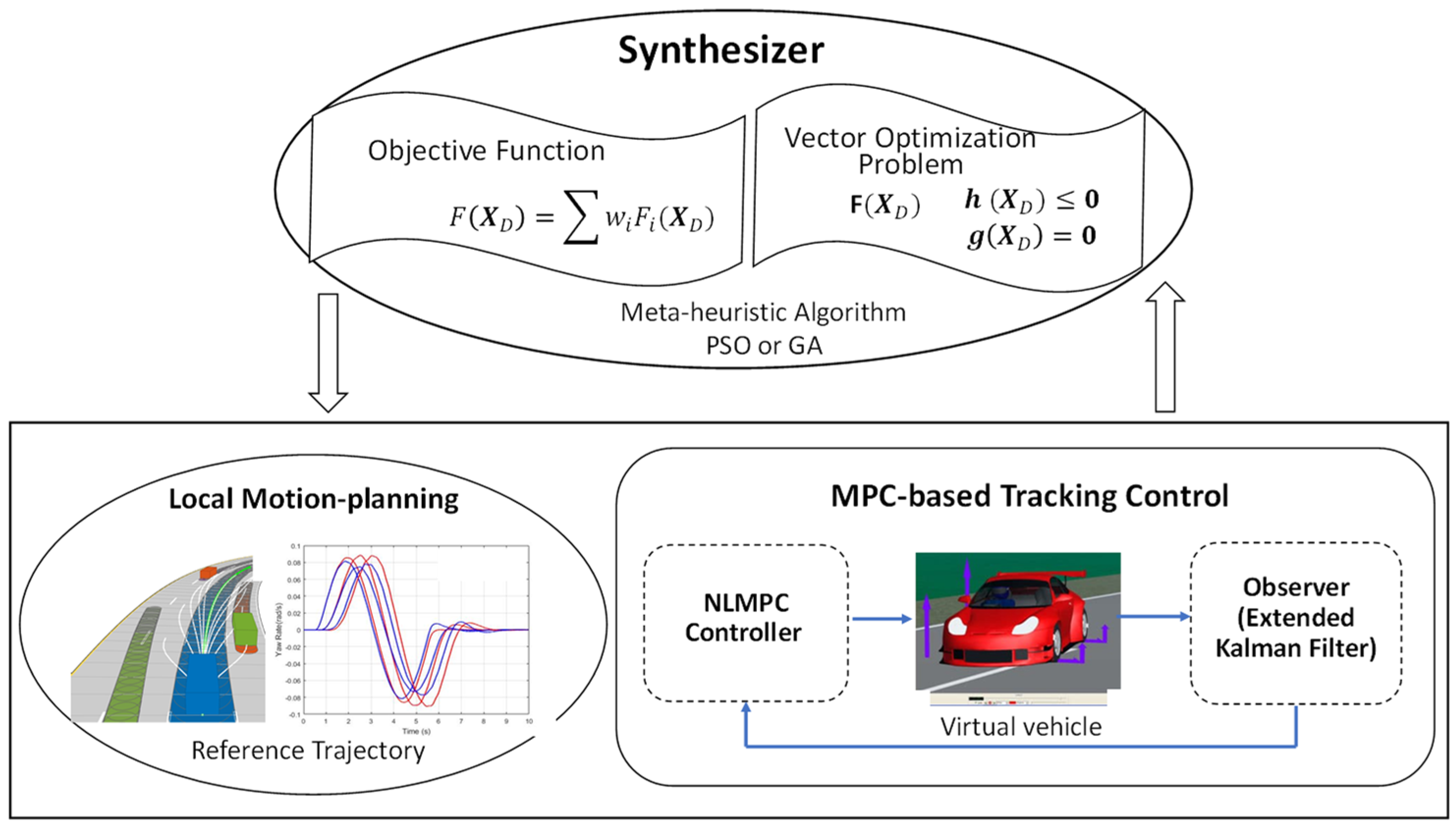
2. Design Methodology

The proposed design method for AVs is shown in Figure 1. This method features a framework with two layers: at the lower layer are the coupled local motion-planning and tracking-control modules; at the upper layer is a design synthesizer.
Given the design variable set X D and constraints at the upper layer, the local motion-planning module and the MPC-based tracking-control module, including the NLMPC controller and the plant (e.g., a vehicle model), are updated. With the data from forward-looking sensors and the behavioral-planning, the local motion-planning is carried out. The identified road boundaries, which take into account various path features and hazard factors, establish constraints on projected vehicle location and orientation. The target trajectory is generated by the motion-planner and the NLMPC controller calculates the desired control inputs to drive the virtual vehicle and track the target trajectory for optimal performance. Via the coupled dynamic analysis between the two modules through closed-loop simulations, the resulting data are sent back to the upper layer. Then, the objective function values and constraints are assessed at the upper layer. The acquired objective function values, F X D , and constraints, h X D 0 and g X D = 0 , are constructed as a vector optimization problem. With a scalarization approach, the vector problem is converted to a scalar one with an objective function taking the form of w i F i X D , where w i ,   i { 1 ,   2 ,   , n } are weights. The design variable set X D may include subsets of X D t , X D m , and X D v , which characterize and represent the target trajectories ( X D t ) , e.g., the tuning parameters for the parametric trajectories defined in [18], the MPC controller ( X D m ) , i.e., the tuning parameters introduced in Section 1, and the mechanical vehicle ( X D v ) , e.g., geometric and inertial parameters of the vehicle, respectively. The formulation of the objective function is discussed in Section 6.
As introduced in Section 1, the MPC-based tracking-control itself is an optimization problem. Thus, the design synthesis shown in Figure 1 is a two-layer optimization problem. Using a two-layer optimization technique for the design of mechatronic vehicles usually leads to a complex nonconvex optimization problem, where a variation of the initial conditions may result in different design solutions [19]. Nevertheless, such a situation can be attenuated by using meta-heuristic search algorithms, e.g., GA and PSO, which have been preferred over gradient-based techniques. In this research, a PSO algorithm was used to solve the upper layer optimization problem shown in Figure 1.

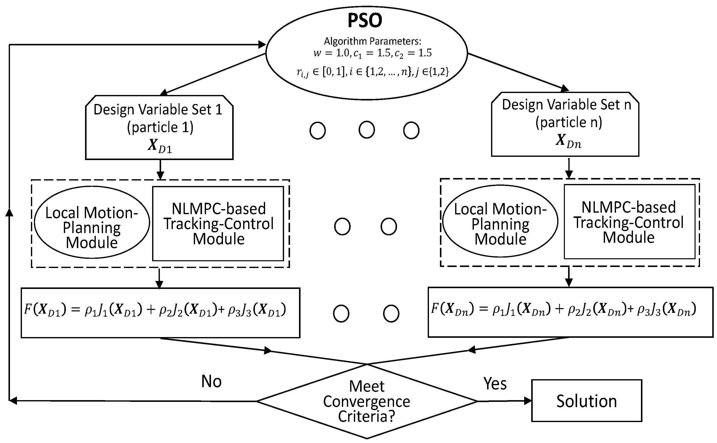
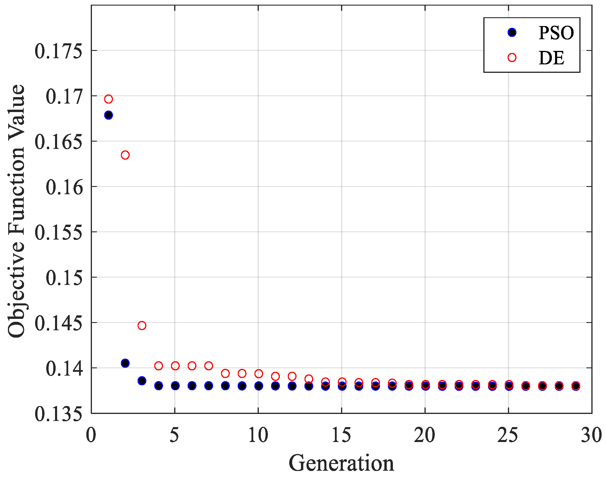
3. Particle Swarm Optimization (PSO) Algorithm

PSO is a meta-heuristic search technique inspired by the choreography of a bird flock [18]. This technique uses a swarm of volumeless particles, which ‘fly’ through a multi-dimensional search space to find the global minimum of an objective function. The flying trajectory of each particle is governed by a simple rule, which considers the current particle velocity and explores the histories of the particle and its neighbors. Due to its simplicity, flexibility, and reliability, PSO has been applied successfully to a variety of optimization problems. Moreover, PSO is more suitable for multi-objective optimization problems owing to its higher search efficiency compared to evolutionary computations (ECs), among which GAs, evolutionary programming, and evolutionary strategies are well-known examples [20].
Both PSO and ECs are population-based. They operate in a similar way, through which these algorithms update their populations using some types of operators based on the fitness information attained; thus, the individuals of the populations are expected to move towards better solution areas in the respective search spaces. To update individuals in the population, ECs usually use two types of operators, including selection and mutation. With a selection operator, poorly performing individuals are removed and are replaced with copies of other population members, namely parents. In ECs, mutation operations take different forms, e.g., crossover. By means of a mutation operator, an EC randomly varies a subset of the individuals in the population. Unlike ECs, the selection operation is not implemented in PSO [20]. Each particle in PSO remains in the population with all population manipulating operations. The updating of individuals in PSO is similar to the use of a crossover operator in ECs. However, the mutation mechanisms used in these techniques are different. In PSO, every particle, i.e., each individual, is updated in accordance with its own flying experience and the swarm’s experience.
A PSO algorithm is used for the upper layer optimization problem shown in Figure 1. Given a D-dimensional search space, the ith particle in the swarm is denoted by Z D , i = z i 1 ,   z i 2 ,   ,   z i D ; the velocity of the particle is represented by V i = v i 1 , v i 2 , , v i D ; P i = p i 1 ,   p i 2 ,   ,   p i D is the position in the search space visited so far by this individual, which provides the best fitness value, i.e., the minimum fitness value, and this position is called the personal best for the individual; P g = p g i , p g 2 , , p g D is the position in the search space visited so far by the gth particle, which gives the minimum fitness value among all the particles in the population, and this position of the gth particle is called the global best for all the individuals of the population. In the PSO algorithm, the particles are updated using the following equations:
v i d k + 1 = w · v i d k + c 1 · r i , 1 · p i d z i d k + c 2 · r i , 2 · p g d z i d k ,   d { 1 , 2 , , D }
z i d k + 1 = z i d k + v i d k + 1
where k + 1 is the total number of updating the particle swarm so far, i.e., the generation number, w the inertia weight, c 1 and c 2 denote two positive constants, and r i , j 0,1 ,     j 1,2 , are random and independent sequences employed to enhance the stochastic nature of the PSO algorithm. As shown in Equation (1), the velocity v i d is updated towards p i d and p g d , weighted by constants c 1 and c 2 , with randomness induced by r i , 1 and r i , 2 , respectively; the inertia weight, w, poses its impact on a local or global search of the PSO algorithm. A large inertia weight is in favor of a global search, while a small inertia weight facilitates a local search.

4. Vehicle System Models

This section introduces two vehicle models, i.e., a nonlinear yaw-plane vehicle model with 2 degrees of freedom (DOF) and a three-dimensional (3-D) vehicle model generated using CarSim software [21]. The 2-DOF yaw-plane model is used to devise the NLMPC controller and to perform the corresponding design optimization, while the CarSim model is utilized for the co-simulation evaluation of the optimal AV designs.

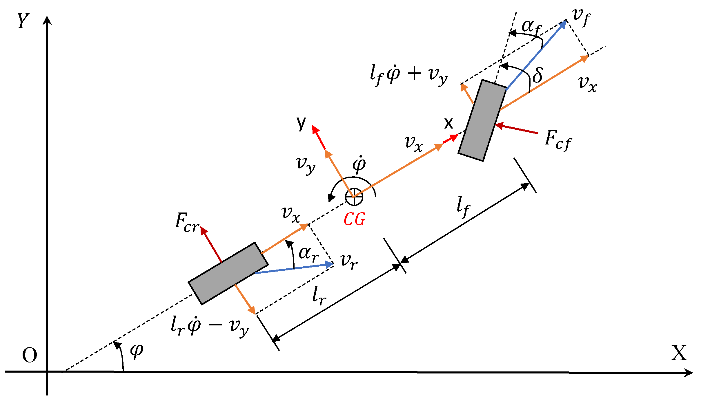
4.1. 2-DOF Nonlinear Yaw-Plane Vehicle Model

Figure 2 shows the single-track model to simulate the lateral dynamics of the vehicle [10,12]. The vehicle system is telescoped laterally, and each axle set is represented by one wheel. Two coordinate systems are the inertial coordinate system, X O Y , and the vehicle body fixed coordinate system, x o y . For the latter, the origin, o, is located at the center of gravity (CG) of the vehicle. The notation of the vehicle model is given in Figure 2.
To derive the vehicle model, we make the following assumptions: (1) vehicle forward speed v x remains constant; (2) given a constant speed v x , tire longitudinal forces and vehicle aerodynamic drag are neglected; (3) vehicle mass is lumped at the CG with a moment of inertia about the vertical axis, z ; and (4) vertical, roll, and pitch motions are neglected. The motions considered are vehicle lateral velocity and yaw-rate, i.e., v y and φ ˙ . Based on Newton’s law of dynamics, the equations of motion of the vehicle are expressed as
m v ˙ y + v x φ ˙ = F c f c o s δ + F c r
I φ ¨ = l f F c f c o s δ l r F c r
where m and I are the vehicle mass and moment of inertia about z axis, respectively, F c f and F c r are the cornering force of the front and rear tire, accordingly, l f and l r the respective distance from the CG to the front and rear axle, and δ is the front wheel steer angle. Note that as shown in Figure 2, v f and v r denote the velocity at the center of the contact area of the front and rear wheel with the road, respectively. Using the ‘Magic Formula’ tire model by Pacejka [22], the tire cornering forces are determined by
F c i = f c i α i , μ , F z i ,   i f , r
where i f , r denotes the front or rear tire, α i the front or rear tire slip angle, μ the friction coefficient between the tire and the road, and F z i the vertical load on the front or rear wheel. As shown in Figure 2, the tire slip angles are given by
α f = δ l f φ ˙ + v y v x α r = l r φ ˙ v y v x
The vertical load on the front and rear wheels is determined by
F z f = m g l r l f + l r F z r = m g l f l f + l r
Under an operating condition with a steer angle input δ and at a constant speed, Equations (3) to (7) determine the lateral dynamic responses of the vehicle.
It is assumed that the vehicle tracks a target path as shown in Figure 3. At an arbitrary instant, point S is the closest point on the path to the vehicle CG, which is located on the normal axis of the n-S-t coordinate system. The tangent line of the target path at point S is determined by angle φ r e f , which is measured in the inertial coordinate system. The orientation of the vehicle is specified by its heading angle φ . At the given instant, the position and orientation of the vehicle with respect to the target path can be determined by
e 1 = φ φ r e f
e ˙ 2 = v y cos e 1 + v x sin e 1 .
where e 1 denotes the vehicle yaw angle error with respect to the target path, and e 2 the vehicle lateral path deviation.
In the inertial coordinate system, the velocities at the vehicle CG are corelated with the heading angle and the velocities measured in the vehicle coordinate system by
X ˙ = v x c o s φ v y s i n φ Y ˙ = v x s i n φ + v y c o s φ
Equations (3) to (10) can be rewritten in the compact form as follows
x ˙ t = f x t ,   u t
where the state and input vectors are defined as x t = v y   φ ˙   φ   e 1   e 2   X   Y T and u t = δ t , respectively.

4.2. CarSim Vehicle Model

The 3-D CarSim model consists of a rigid vehicle body, two suspensions, and four wheels. The motions considered include the longitudinal, lateral, vertical, roll, pitch, and yaw motion of the body, as well as the vertical and spinning motions of each wheel. The nonlinear features of vehicle components, e.g., suspensions and pneumatic tires, are mimicked in the model.
In CarSim software, a symbolic multi-body program, called VehicleSim (VS) Lisp, is used to derive equations of motion for vehicle systems [21]. VS Lisp takes an input as the description of the 3-D vehicle model configuration mostly in geometric terms, such as the body DOF, point locations and the directions of force vectors. With the input information, VS Lisp generates equations of motion in terms of ordinary differential equations and produces a source code (C or Fortran) to solve them.
CarSim software involves three key components: VS browser, CarSim databases, and VS solver. The VS browser is a graphical user interface. The CarSim databases are used to choose vehicle configuration templates, e.g., dependent or independent suspension, and to define the system parameters, the tire/road interactions, the test maneuvers, etc. The VS solver is used to solve the derived governing equations of motion and to execute the defined simulations. The VS browser can also be applied to other applications, e.g., incorporating the NLMPC controller to be designed into Matlab/Simulink in the 3-D vehicle model via an interface for co-simulation.

5. NLMPC Controller Design

As shown in Figure 1, at the lower layer of the design synthesis are the coupled components of the motion-planner, NLMPC controller, and virtual vehicle. This section introduces the design of the NLMPC controller and outlines the local motion-planning method.

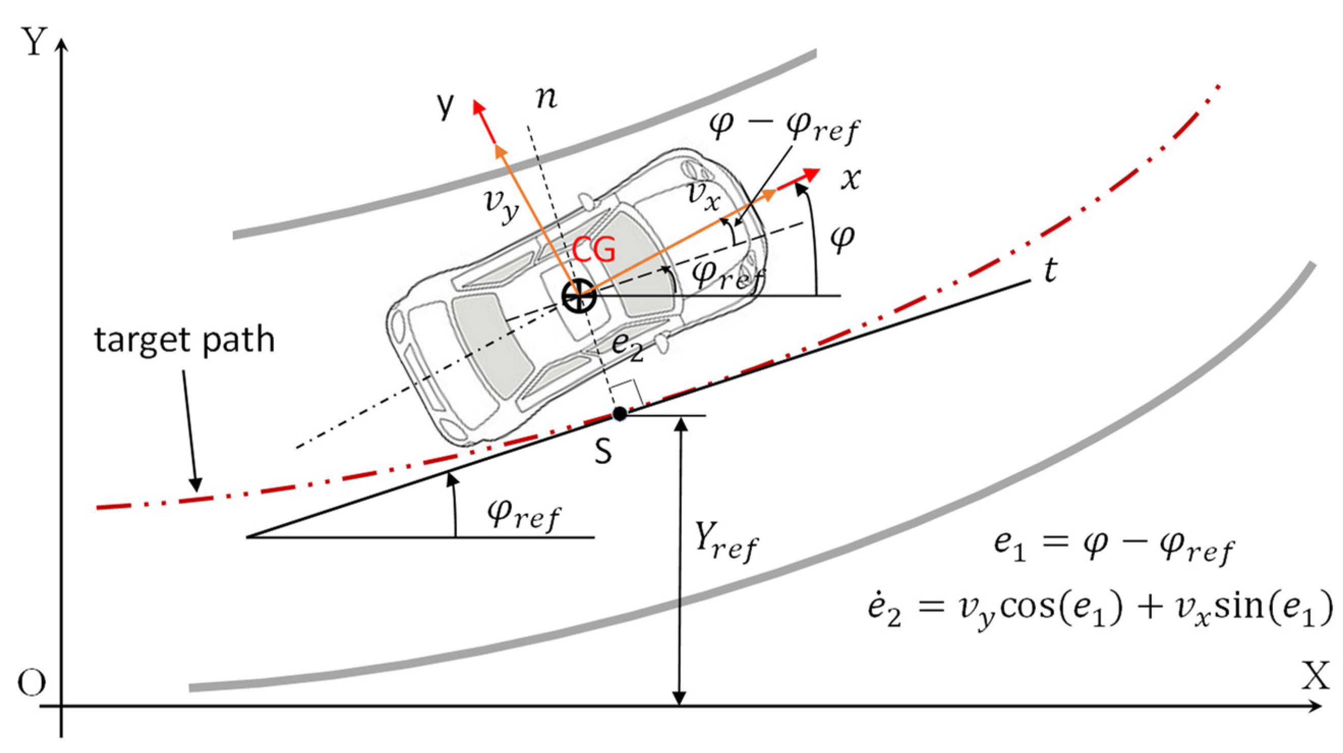
5.1. Tracking Controller Design

The NLMPC controller consists of two core elements: the discretized vehicle model derived from Equation (11), and an optimizer with a cost function and a batch of constraints. The discretized model is used to derive a prediction of future output vehicle dynamic behavior. With the prediction, optimization is conducted to find a sequence of control input moves, which minimizes the selected measures of the output deviation from their respective reference trajectories, while satisfying all the given constraints. To improve the quality of prediction, adequate measurements are collected; however, only the first of the calculated control input sequences is implemented. The optimization is repeated at the next sampling time. This ‘receding horizon implementation’ makes the MPC algorithm a feedback controller.
At sampling step k , discretizing the nonlinear vehicle model represented by Equation (11) with the forward Euler method leads to
x k + 1 = f x k , u k
u k = u k 1 + u k .
where x k = v y ( k )   φ ˙ ( k )   φ ( k )   e 1 ( k )   e 2 ( k )   X ( k )   Y ( k ) T , u k = δ k , u k = δ k , and y k denotes the output variable vector determined by
y k = C x k = 0 0 1 0 0 0 0 0 0 0 0 0 0 1 x k
It is assumed that the reference trajectory is defined as
r k = [ φ r e f k   Y r e f ( k ) ] T
Considering the control input, output variable vector, and the desired outputs specified by Equations (13)–(15), respectively, we formulate the NLMPC controller design as an optimization problem with the following cost function subject to the specified constraints
min u k k , , u k + H c 1 k J x k , u k = i = 1 H p y k + i k r k + i k Q 2 + i = 0 H c 1 u k + i k R 2
x k + 1 + i k = f x k + i k , u k + i k ,   i { 0 , , H p 1 }
u k + i k = u k 1 + i k + u k + i k ,   i { 0 , , H p 1 }
y k + i k = C x k + i k ,   i { 1 , , H p }
δ m i n u k + i k δ m a x ,   i { 0 , , H c 1 }
u k + i k = 0 ,   i { H c , , H p 1 }
where the symbol k indicates the sampling step k , at which the control input u k is given for the closed-loop control of vehicle plant, H p and H c are the prediction and the control horizon, respectively, Q R 2 × 2 and R R 1 × 1 are the matrices corresponding to weights on the output and control input vectors, accordingly, u k = [ u ( k k ) , , u ( k + H c 1 ) k ] T denote the predicted control input series at time series of k , , k + H c 1 , and y k + i k the output vector predicted at time k + i attained by starting from the state vector x k . Note that H p > H c , and the predicted control inputs are assumed constant in the time interval from H c to H p .
In Equation (16a), the first summand imposes the penalty on trajectory tracking deviation, while the second summand is to prevent large control effort for the automated steering. Solving the optimization problem described in Equation (16), we obtain the optimal control input increments evaluated at the sampling step k for the currently observed vehicle state vector x k , and denote the optimally predicted control input increments by
u * k [ u * ( k k ) , , u * ( k + H c 1 ) k ] T
where the first control input increment is used to update the required control action as described in Equation (13). The resulting state feedback control law is thus cast as
u k + 1 = u k + u * k k
At the next sampling step k + 1 , the control action u k + 1 is applied to the vehicle plant to acquire the new vehicle state vector x k + 1 , with which the optimization problem Equation (16) is to be solved again over a shifted horizon.
To summarize the design of the NLMPC controller, we visualize the interrelations between the controller and the vehicle plant using the block diagram shown in Figure 4.

5.2. Reference Trajectory

In the operation of motion-planning module, with the global route determined by the route planner, the behavioral planner decides on a local driving task with a motion specification. Following the directives of the behavioral planner, the local motion-planner generates the reference trajectory (i.e., r · ) for the NLMPC controller to track, as shown in Figure 4.
To date, studies have been conducted to explore techniques for local motion-planning. These techniques may be classified into two groups [23]: (1) separated methods, by which spatial maneuver (e.g., a single lane-change (SLC) for obstacle avoidance at a constant forward speed) and temporal maneuver (e.g., speeding up along a predefined SLC path to overtake a front vehicle) are separately planned; (2) integrated approaches, with which the spatial and temporal maneuvers are planned simultaneously. The integrated techniques exhibit poor performance in terms of computational efficiency. In contrast, the separated methods significantly improve computational efficiency due to the layered nature [24].
In this research, the separate methods were adopted. Due to the fact that only autonomous steering control at a constant forward speed was considered in this study, the local motion-planning was reduced to a path planning problem. It is indicated that the testing maneuver with a single cycle sine wave steering input is well-accepted for assessing road vehicles’ handling performance in terms of path-following and yaw stability under an SLC maneuver at a constant forward speed [25]. To facilitate systematic and repeatable tests of the proposed design synthesis method, it was assumed that the local motion-planning results in an SLC path at a given speed. Under the evasive maneuver, the vehicle with automated steering was evaluated in terms of path-following, yaw stability, and driving quality.

6. Design Synthesis Problem Formulation and Implementation

The design of the vehicle with automated steering was conducted with the proposed framework. This section outlines the design in terms of: (1) design objectives, variables, and constraints, and (2) design synthesis implementation.

6.1. Design Objectives, Variables, and Constraints

The design of the vehicle with automated steering aimed at improving path-following, ensuring yaw stability, and enhancing ride quality under severe operating conditions. To this end, obstacle avoidance maneuvers in highway and urban area operations are simulated. It is assumed that, under these SLC maneuvers, the paths to be tracked by the AV are determined by the motion-planner. Under each SLC maneuver, the AV follows the path at a constant forward speed, v x . Under the maneuver, the NLMPC controller adjusts the steering angle, δ , to improve path-following, ensure yaw stability, and enhance ride quality by minimizing the path-following off-tracking, J 1 , yaw angle deviation, J 2 , and the ride quality measure, J 3 .
As shown in Figure 3, the target path can be defined by the lateral position, Y r e f t , and the tangential angle, φ r e f t , of the path at point S; the path-following off-tracking of the AV is directly associated with the vehicle lateral path deviation ( e 2 ) defined by Equation (9); the yaw angle deviation of the AV is related to the vehicle yaw angle error e 1 specified by Equation (8); the ride quality of the AV is determined by the lateral acceleration of the vehicle, a y = v ˙ y + v x φ . Over the SLC maneuver, the forward speed ( v x ) remains constant. Assuming the time duration for completing the SLC maneuver is T s l c , we define the path-following off-tracking performance measure as
J 1 = 1 T s l c 0 T s l c e 2 t 2 d t 1 2
where J 1 represents the root of mean square (RMS) value of the vehicle lateral path deviation, e 2 , over the SLC maneuver.
Similarly, the yaw angle deviation of the AV is specified as
J 2 = 1 T s l c 0 T s l c e 1 t 2 d t 1 2
where J 2 denotes the RMS value of the vehicle yaw angle error, e 1 , over the SLC maneuver.
Finally, the ride quality measure is determined by
J 3 = 1 T s l c 0 T s l c a y t 2 d t 1 2
where J 3 represents the RMS value of the vehicle’s lateral acceleration, a y , over the maneuver. A quantitative assessment of the ride quality can be performed with the respective measures by ISO-2631-1 [26], which specifies metrics to quantify the evaluation of human exposure to whole-body vibration in relation to vehicle occupant health and comfort, probability of vibration perception and incidence of motion sickness. This research considers one index, i.e., an acceleration along the y axis ( a e q , y ). This index corresponds to the performance measure J 3 . The evaluation of the ride comfort based on a e q , y is attained by examining the approximate human reactions at various magnitudes of the equivalent RMS values of acceleration provided by ISO-2631-1, which are presented in Table 1.
For the optimization problem, the design variable set X D comprises two subsets: X D m and X D v , representing the tuning parameters of the NLMPC controller, as well as the geometric and inertial parameters of the mechanical vehicle, respectively.
In the designs of MPC controllers, the tuning parameters frequently involve [16] the prediction horizon, H p , control horizon, H c , sample time, T s , output weighting matrix Q , and control input variation weighting matrix R . In real-time implementation of MPC controls, practical limitations usually restrict the availability of sample time, T s , as a tuning parameter. In the designs of MPC controllers for AVs, it is suggested that sample time, T s , take 0.05 s [10]. This study adopted the recommended sample time. Reliable guidelines for selecting the tuning parameters of the prediction horizon, H p , and control horizon, H c , are well established [16]. Following these guidelines, this research made a reliable selection, i.e., H p = 20 , and H c = 10 .
It was indicated that the selection of output weighting Q and control input variation weighting R are still open to discussion [16]. With the above considerations, we treat the elements of the weighting matrices Q and R as the components of the design variable subset X D m . In the design synthesis, the NLMPC controller design is formulated as the lower-layer optimization problem expressed in Equation (18). The vectors of output, reference output, and control input variation are specified as
y k = φ ( k ) Y ( k ) T
r k = φ r e f ( k ) Y r e f ( k ) T
u k = δ k
With the vectors of output, reference output, and control input variation defined in Equation (24), the weighting matrix Q R 2 × 2 and R R 1 × 1 are reduced to
Q = q 1 0 0 q 2
R = R
Thus, the design variable subset X D m is defined as
X D m = q 1 q 2 R
Among various geometric and inertial parameters of road vehicles, total mass m , wheelbase l , and distance from vehicle CG to the front axle l f are directly associated with path-following capability, yaw stability, and ride quality under severe evasive maneuvers [27]. In this research, these three parameters constitute the mechanical vehicle design variable subset X D v , which is specified as
X D v = m l l f
In the design synthesis, the evaluations of the performance measures defined by Equations (19) to (21) are attained based on the dynamic responses of the vehicle plant (defined by Equation (11)) over the simulated SLC maneuver. The design variable subsets, X D m and X D v , are allowed to vary from their lower bounds ( X D m l and X D v l ) to the respective upper bounds ( X D m u and X D v u ). Following the design framework shown in Figure 1, the upper layer optimization problem is formulated to realize the aforementioned design objectives subject to the specified constraints. The formulation is constructed as
min X Dm , X Dv F X D = i = 0 3 ρ i J i X D
subject to:
x ˙ t = f x t ,   u t
X D m l , i X D m , i X D m u , i ,   i { 1,2 , 3 }
X D v l , i X D v , i X D v u , i ,   i { 1,2 , 3 }
where ρ 1 , ρ 2 , and ρ 3 are the normalized weighting factors for the vehicle performance measures, J 1 , J 2 , and J 3 , respectively; Equation (26b) defines the nonlinear vehicle model, by which the objective function and constraints are evaluated; X D m , 1 , X D m , 2 , and X D m , 3 denote q 1 , q 2 , and R , while X D m l , i and X D m u , i , i { 1,2 , 3 } are the lower and upper bounds of the respective design variables X D m , i ; X D v , 1 , X D v , 2 , and X D v , 3 represent m , l , and l f , while X D v l , i and X D v u , i ,   i { 1,2 , 3 } are the lower and upper bounds of these vehicle design variables, respectively.
To facilitate the design optimization, every term on the right-hand side of Equation (26a) is normalized using the corresponding norm [13]. In the case concerned, the norm of each term is the inverse of the corresponding weighting factor, that is,
ρ i = 1 / J i n o r m ,   i { 1,2 , 3 }
where J i n o r m are the performance measures defined and calculated using Equations (19) to (21), respectively, with the design variables taking their nominal values, which will be provided in Section 7.

6.2. Two-Layer Optimization Problem Implementation

As illustrated in Figure 5, to run the PSO algorithm, the undetermined parameters in Equation (1) are assigned finely tuned values: w = 1.0 , c 1 = 1.5 , c 2 = 1.5 , and the total number of particles is n. In the case concerned, the number of design variables is six.
Initially, the PSO algorithm stochastically chooses n designs in the 6-dimensional design variable space. Subsequently, each design X D i ,   i { 1,2 , , n } is delivered to the coupled local motion-planning and NLMPC tracking-control modules. With a given design variable set, X D i , as shown in Figure 4, the specified geometric and inertial parameters of the vehicle model and the tuning weights of the NLMPC controller are updated. Under an SLC maneuver, the reference path for the AV is determined by the local motion-planning module. Over the SLC maneuver, the NLMPC controller determines the steering angle δ of the vehicle plant to track the reference path at a constant speed. After completing the SLC maneuver, a fitness value, F X D i = j = 1 3 ρ j J j X D i , i { 1,2 ,   ,   n } , can be derived using the dynamic responses of the vehicle plant over the SLC maneuver.
With the execution of the equivalent SLC maneuver corresponding to each of the n design variable sets, a fitness value vector, F X D 1 ,   F X D 2 ,   ,   F X D n   , is obtained. At this point, if the convergence criteria, e.g., a predefined total generation number, an acceptable error between the best fitness values of the last two generations, etc., are satisfied, the optimization process terminates. Otherwise, the achieved fitness value vector is feedbacked to the PSO at the upper layer. Based on the returned fitness value vector corresponding to the given design variable sets, the PSO creates the next generation of design variable sets (or particles) using the ‘particles’ updating operator defined in Equations (1) and (2). This process repeats until the optimal design variable set is found.

7. Results and Discussion

The two-layer design optimization shown in Figure 5 is implemented considering two operating scenarios: 1) urban, and 2) highway. In each of the scenarios, the respective SLC maneuver by ISO-14791 is simulated, and the reference path is prescribed [28]. These reference paths are mathematically defined by
Y X = ( X / V x ) ( T / 2 π ) sin ( 2 π X / T V x ) · ( L / T )
where X and Y denote the horizontal and vertical displacement (in meters) of a point on the target path displayed in the inertial reference frame, V x   (in m/s) is vehicle forward speed, L (in meters) is the maximum SLC lateral displacement, and T (in seconds) is the time duration. For the two scenarios, the values of the reference path parameters are provided in Table 2.
To implement the optimization, we select the nominal values, as well as the lower and upper bound values of the design variables, which are listed in Table 3. Note that the design optimization is implemented independently in the two scenarios, i.e., urban and highway. For implementing these design optimizations, both the population number (i.e., the total number of particles), n, and the total number of generations of the PSO algorithm are assigned the value of 100.
After the execution of the design optimizations under the two operating scenarios, the optimal design variable sets and the respective performance measures defined in Equations (19) to (21) are attained. The resulting values of the optimal design variables are also provided in Table 3.
To analyze and evaluate the attained optimization results, we conducted co-simulations by integrating the virtual vehicle, i.e., the CarSim model, with the coupled motion-planning and NLMPC tracking-control modules designed in Matlab. The co-simulations are performed using the similar technique introduced in [29]. In our co-simulations, the urban and highway SLC maneuvers are simulated; in the urban and highway operating scenarios, the NLMPC controller and the vehicle models take the respective nominal and optimal design variable values listed in Table 3. In the following subsections, we first examine the co-simulation results in terms of the performance measures of the nominal and optimal designs in both the urban and highway scenarios, then evaluate the effects of optimal design variables on the performance improvements.
Note that this paper presents the preliminary research results to examine the proposed design method shown in Figure 1 and Figure 5. In this preliminary research phase, considering the cost and safety concerns, it may not be practical to conduct field or road tests to evaluate the proposed design method. Nowadays, vehicle modeling and simulation are of importance for vehicle design and development. Simulation is increasingly used in the design and testing of vehicles in a virtual environment prior to a physical full-size vehicle prototype being fabricated [30]. In Australia, the performance-based standards for articulated vehicles, both in-vehicle tests and simulations, are permitted to evaluate the lateral dynamics of these vehicles [31]. This section thus presents only numerical simulation results to evaluate the proposed design method.

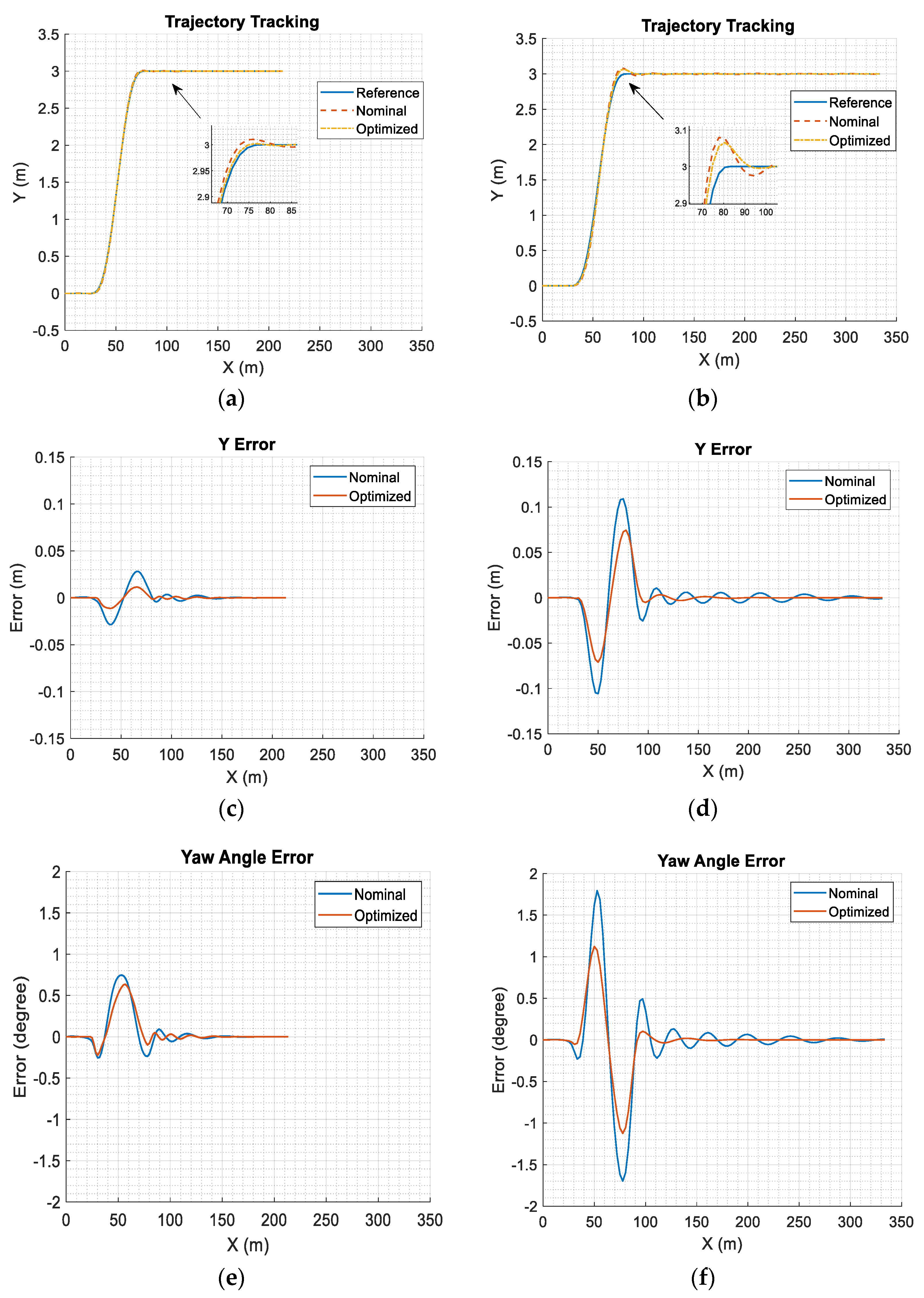
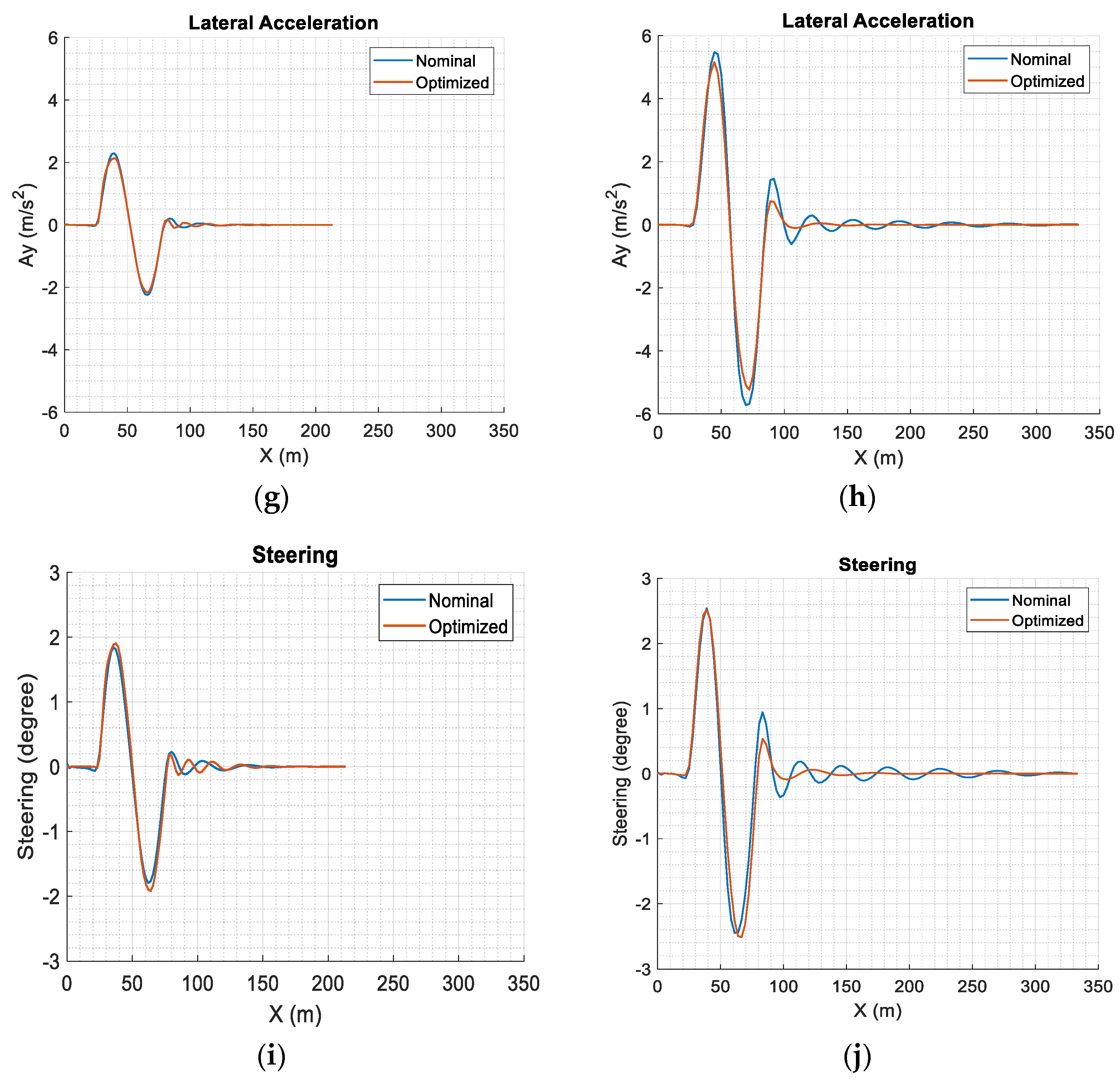
7.1. Performance Measures

In the urban scenario, the nominal and optimal designs are compared and evaluated, as shown in Figure 6a,c,e,g,i. Figure 6a shows the reference path and the trajectories of the vehicle CG for the nominal and optimal designs. It seems difficult to distinguish the differences among the three paths without the aid of the focused and enlarged windows accompanying the figure. By means of the accompanying window in the figure, we observe the fact that the path of the optimal design is closer to the reference one with a lower overshoot compared to the counterpart of the nominal design. The simulation results illustrated in Figure 6c,e justify our observation. As shown in Figure 6c, in the nominal design, the maximum peak lateral position deviation of the vehicle CG from the reference path Y e r r _ M a x is 0.0287 m; while in the optimal design, this measure is 0.0115 m, decreasing by 59.9% from the counterpart of the nominal design. Figure 6e shows that in the optimal design, the maximum peak vehicle yaw angle deviation from the reference value Y a w _ a n g e r r _ M a x is 0.6357°, reducing by 14.8% from the corresponding measure of 0.7462° for the nominal design.
Figure 6g displays the vehicle dynamic response in terms of the variation of the lateral acceleration at the vehicle CG in both the nominal and optimal designs. Obviously, the fluctuation of the lateral acceleration in the nominal design is more violent with larger peak values than its counterpart in the optimal design. To evaluate the ride comfort of the designs, RMS values of lateral acceleration ( a y ) over the SLC maneuver are calculated using Equation (21). In the optimal design, this measure takes the value of 0.7599 m / s 2 , reducing by 3.1% from its nominal value of 0.7845 m / s 2 . Assessing the ride quality based on the ISO-2631-1 specifications listed in Table 1 we find that for both the optimal and nominal designs, the vehicle occupants will feel fairly uncomfortable during the urban SLC maneuver.
Figure 6i displays the front wheel steering angle input controlled by the corresponding NLMPC controller during the SLC maneuver for each of the two designs. As expected, each of the steer inputs took a single cycle sine waveform for the SLC maneuvers. It was found that with the approximate same time period, the two sine wave inputs had different amplitudes. For the optimal design, the maximum amplitude S t e e r _ a n g M a x was 1.9201°, which was increased by 4.2% from its nominal value of 1.8425°. It was found that for a given SLC maneuver, the total area (absolute value) enclosed by the vehicle front-wheel steer angle curve and the horizontal axis may be viewed as an indicator for steering control effort [32]. A close observation of Figure 6i discloses that the overall steering control effort of the optimal design was larger than its counterpart of the nominal design.
All the aforementioned performance measures of the nominal and optimal designs, as well as their relative variations, are listed in Table 4. The above analysis indicates that the optimal design outperformed the nominal one in the performance measures of path-following off-tracking, yaw angle deviation, and ride quality. The performance improvement of the optimal design may be attributed to its larger steering control effort of the front wheel.
In the case of the highway scenario, the respective performance measures of the nominal and optimal designs are also provided in Table 4. Interestingly, the performance improvement of the optimal design over the nominal design in the highway scenario was similar to that in the urban scenario. To dig out the root causes leading to these performance improvements, the following subsection analyzes the effects of design variables and justifies the optimal designs.

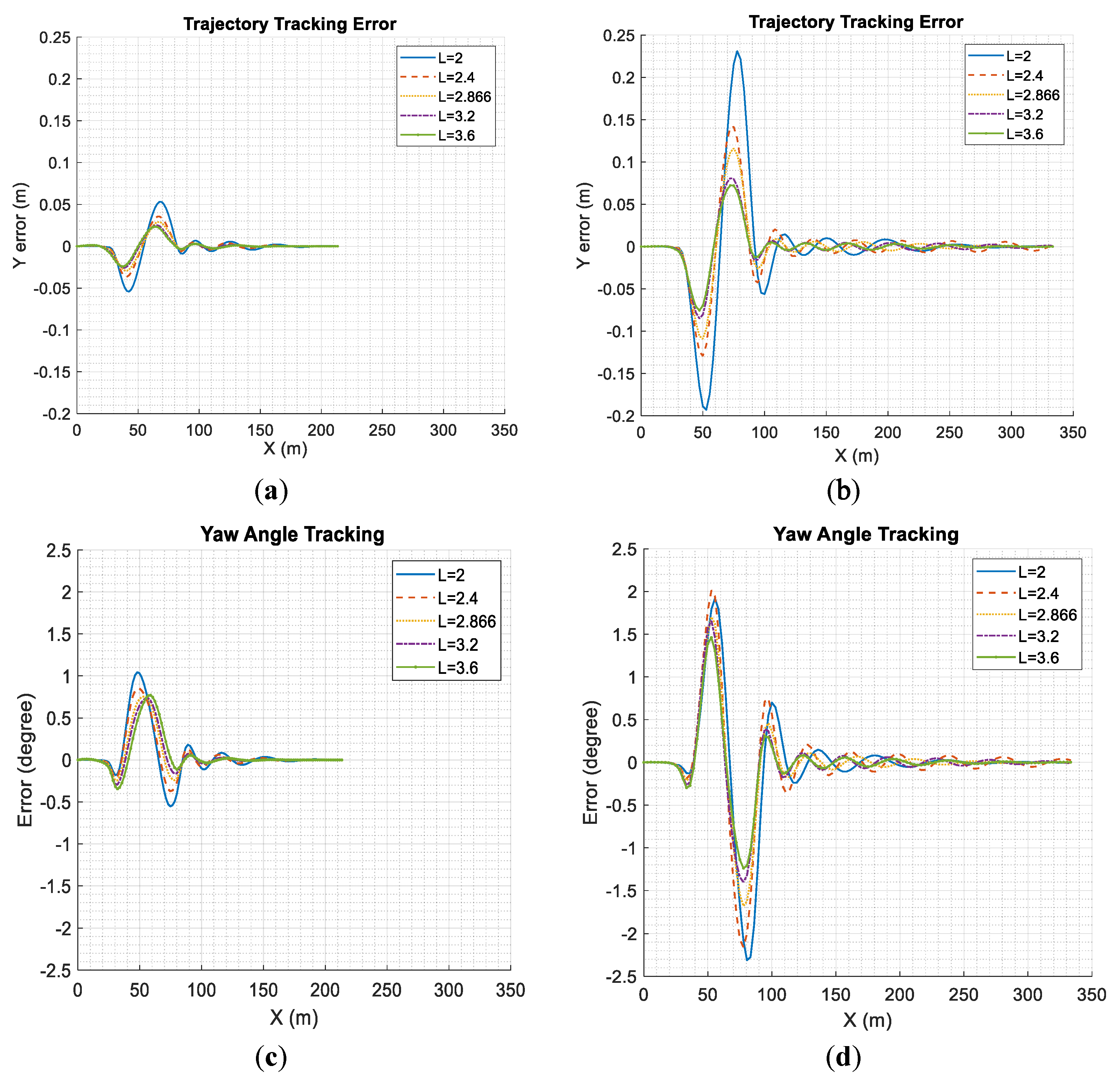
7.2. Effects of Design Variables

To make the article concise, we only selected two design variables, i.e., l (vehicle wheelbase) and q 1 (weight on yaw angle deviation), and evaluated the impacts of each of the two variables on the performance measures of Y e r r (vehicle CG lateral position deviation from the reference path) and Y a w _ a n g e r r (vehicle yaw angle deviation from the reference angle). In the following sensitivity analysis for evaluating the effects of the selected design variables, for each case study, only the chosen design variable varied, while others remained fixed with their nominal values provided in Table 3. The simulation results for the sensitivity analysis were derived from the simulated urban SLC (USLC) maneuver and the highway SLC (HSLC) maneuver.
Figure 7a,b illustrates the impact of l on Y e r r in the USLC and HSLC, respectively. It was found that in both scenarios, the maximum peak Y e r r value decreased with the increase in l value. It appears that a larger l achieved a better measure of Y e r r . Figure 7c,d shows the influence of l on Y a w _ a n g e r r . In the HSLC case, a larger l also achieved a better measure of Y a w _ a n g e r r . A close observation of Figure 7d reveals that the larger the l value becomes, the smaller the maximum peak Y a w _ a n g e r r value will be attained. This observation may explain why in the HSLC case, the optimal l takes the value of 3.55 m, which was very close to the upper bound value of 3.6 m.
However, in the USLC case as shown in Figure 7c, the above conclusion derived from the observation based on the result illustrated in Figure 7d was not true. As seen in Figure 7c, when the vehicle wheelbase l took the value of 3.6, 3.2, and 2.866 m, the corresponding maximum peak Y a w _ a n g e r r values were 0.7702°, 0.7346°, and 0.7462°. The above values of l and the respective maximum peak Y a w _ a n g e r r values were not consistent with the aforementioned observation, that is, ‘the larger the l value becomes, the smaller the maximum peak Y a w _ a n g e r r value will attain’. Interestingly, among the above three listed l values, the one with the value of 3.2 m led to the Y a w _ a n g e r r measure of 0.7346°, which was the least among the three measures. The l value of 3.2 m was very close to the optimized value of 3.16 m listed in Table 3.
The above analysis regarding the effect of l on the measures of Y e r r and Y a w _ a n g e r r discloses that as vehicle forward speed increases, a longer wheelbase benefits for decreasing the cross path error and enhancing yaw stability. This observation is consistent with the conclusion reported in [19] where a shorter wheelbase is advantageous to achieving a better low-speed (less than 15 km/h) path-following performance, while in high-speed evasive maneuvers, an ideal wheelbase value selection is a trade-off solution between transient path-following off-tracking and yaw/lateral stability. The aforementioned sensitivity and dynamic analysis effectively explain the optimal wheelbase value for the USLC and HSLC scenarios.
Figure 8a,b displays the effect of q 1 on Y e r r in the USLC and HSLC, accordingly. In the USLC case, the influence of q 1 on the peak values of Y e r r was weak. This is reflected by the curves shown in Figure 8a. It is shown that with the variation of q 1 , the change in the two peak values of Y e r r was not evident. In the HSLC case (as shown in Figure 8b), however, it is observed that the larger the weight of q 1 , the larger the maximum peak Y e r r . Based on Equations (15), (16a), (22b), and (23a), we know that q 1 is the weight imposed on the output of Y a w _ a n g e r r . For the weighted-sum method-based multi-objective optimization of the NLMPC problem formulated in (16a) to (16g), with the fixed weights of q 2 and R , increasing the weight of q 1 leads to a heavier penalty on Y a w _ a n g e r r ; in contrast, this results in a relatively lighter penalty on Y e r r . The results shown in Figure 8b visualize the above inference.
Shown in Figure 8c,d are the effects of q 1 on Y a w _ a n g e r r in the USLC and HSLC scenarios, respectively. By means of imposing a penalty on the magnitude of Y a w _ a n g e r r , increasing the weight value of q 1 leads to a decrease in the maximum peak value of this measure in both scenarios. Thus, the measures of Y e r r and Y a w _ a n g e r r pose the contradicted requirements on q 1 in both the cases and, in particular, the HSLC case. An ideal weight of q 1 is, generally, a compromised solution between the conflicting design criteria; the corresponding optimal q 1 will be a value between the lower and upper bound values of 0 and 20. As shown in Table 3, in the USLC case, the optimal value is 4.30, which is smaller than the nominal value, i.e., 15.00, while in the HSLC case, the counterpart is 16.40, which is bigger than the nominal value.
The difference between the optimal values of q 1 in the USLC and HSLC scenarios is consistent with the vehicle design principle proposed in [20] where in low-speed curved road negotiations, emphasis should be placed on improving path-following performance (i.e., lateral position deviation), whereas in high-speed evasive maneuvers, more attention should be paid to ensuring yaw stability (i.e., yaw angle deviation).
In addition to the above sensitivity and vehicle dynamic analysis, we have also evaluated the effects of the other individual design variables, including q 2 , R , m , and l f , on the performance measures of Y e r r , Y a w _ a n g e r r , and the RMS value of a y , respectively. Our comprehensive sensitivity and vehicle dynamic analysis justifies the optimal designs of the road vehicle with autonomous steering functions in both the USLC and HSLC scenarios. The successful implementation of the design optimization demonstrates the effectiveness of the proposed design synthesis method shown in Figure 1.
In this study, the computations were carried out on an HP Pavilion desktop computer with a processor of Intel (R) Core (tm) i7-6700 CPU at 3.4 GHz. To facilitate the evaluation of the performance of the PSO algorithm in solving the upper layer optimization problem expressed in (26), another stochastic search algorithm, i.e., differential evolution (DE) [33], was also used to solve the same problem and its performance is compared with that of the PSO. With six runs of the two-layer optimization seen in Figure 5, both search algorithms individually attained the optimal design listed in Table 3. Figure 9 shows the relation of the values of the objective function specified in (26a) with the generation number in the third run of the DE and PSD. To achieve the provided optimal design, the PSO uses 9.63 min for one generation, while the DE takes 10.96 min; the former’s computation efficiency was 12.1% higher than the latter.

8. Conclusions

Considering the fact that an AV is a complex mechatronic system consisting of multi-subsystems including the mechanical vehicle, motion-planning, tracking-control, etc., this article proposes a two-layer design synthesis method for AVs. At the lower layer, these dynamically coupled subsystems are modeled and synthetized as an integrated AV; the virtual AV is then simulated with the modules of motion-planning and tracking-control to operate in ‘real-time’ under a given operating maneuver. At the upper layer, a multi-objective optimization problem is formulated with the design criteria of path-following off-tracking, lateral/yaw stability, ride comfort, etc. The proposed method aims to find ideal solutions to the complex AV optimization problem to satisfy the specified design requirements and constraints.
To assess the applicability and effectiveness of the proposed method, it is applied to the design synthesis of a road vehicle with an automated steering function. For implementing this design synthesis, a PSO search algorithm is introduced to solve the upper layer optimization problem; at the lower layer, the AV is modeled with the subsystems of a motion-planning, a mechanical vehicle, and an NLMPC tracking-control; an ideal AV design with the optimal design variables of the mechanical vehicle and NLMPC controller is sought under the simulated USLC and HSLC maneuvers. Due to the enlarged design space, including the design variable sets for a mechanical vehicle and a tracking controller, the optimal AV is superior to its nominal design in terms of path-following off-tracking, lateral/yaw stability, and ride quality. The respective sensitivity and dynamic analyses justify the selected optimal design. The case studies presented in the paper disclose the following findings:
(1)
The proposed method can be applied in the early design states for AVs for identifying desired design variables and predicting performance envelops.
(2)
The optimal designs (including optimal tracking-control and vehicle system design variables) for an AV are operating condition-dependent. This implies that in highway and urban operations, distinct optimal design variable sets should be determined, respectively, in order to achieve desired performance envelops.
To improve the proposed design synthesis method, we will enhance the function of tracking-control by introducing vehicle forward speed control, incorporate the perception module in the AV, and further enlarge the design space by adding the design variables for the modules of perception and motion-planning.

Author Contributions

Conceptualization and methodology, C.M. and Y.H.; writing—original draft preparation, C.M.; supervision, Y.H. and M.A.-C.; funding acquisition, Y.H. and M.A.-C. All authors have read and agreed to the published version of the manuscript.

Funding

This research was funded by the Natural Sciences and Engineering Research Council of Canada, grant number RGPIN/2019-05437.

Data Availability Statement

Data are contained within the article.

Acknowledgments

Y.H. would like to thank the team members of the Multidisciplinary Vehicle Systems Design Laboratory, University of Ontario Institute of Technology. These team members have conducted a preliminary study on design methodology for autonomous ground vehicles.

Conflicts of Interest

The authors declare no conflicts of interest.

References

  1. Paden, B.; Čáp, M.; Yong, S.Z.; Yershov, D.; Frazzoli, E. A survey of motion planning and control techniques for self-driving urban vehicles. IEEE Trans. Intell. Veh. 2016, 1, 33–55. [Google Scholar] [CrossRef]
  2. Rosique, F.; Navarro, P.J.; Fernández, C.; Padilla, A. A systematic review of perception system and simulators for autonomous vehicles research. Sensors 2019, 19, 648. [Google Scholar] [CrossRef] [PubMed]
  3. Yeong, D.J.; Velasco-Hernandez, G.; Barry, J.; Walsh, J. Sensor and sensor fusion technology in autonomous vehicles: A review. Sensors 2021, 21, 2140. [Google Scholar] [CrossRef] [PubMed]
  4. Ananda, M.P.; Bernstein, H.; Cunningham, K.E.; Feess, W.A.; Stroud, E.G. Global Positioning System (GPS) autonomous navigation. In Proceedings of the IEEE Symposium on Position Location and Navigation. A Decade of Excellence in the Navigation Sciences, Las Vegas, NV, USA, 20 March 1990; pp. 497–508. [Google Scholar]
  5. Rahiman, W.; Zainal, Z. An overview of development GPS navigation for autonomous car. In Proceedings of the 2013 IEEE 8th Conference on Industrial Electronics and Applications, ICIEA 2013, Melbourne, VIC, Australia, 19–21 June 2013. [Google Scholar]
  6. Mohamed, S.A.S.; Haghbayan, M.H.; Westerlund, T.; Heikkonen, J.; Tenhunen, H.; Plosila, J. A survey on odometry for autonomous navigation systems. IEEE Access 2019, 7, 97466–97486. [Google Scholar] [CrossRef]
  7. Kaminer, I.; Pascoal, A.; Hallberg, E.; Silvestre, C. Trajectory tracking for autonomous vehicles: An integrated approach to guidance and control. J. Guid. Control Dyn. 1998, 21, 29–38. [Google Scholar] [CrossRef]
  8. Kanayama, Y.; Kimura, Y.; Miyazaki, F.; Noguchi, T. A stable tracking control method for an autonomous mobile robot. In Proceedings of the IEEE International Conference on Robotics and Automation, Cincinnati, OH, USA, 13–18 May 1990. [Google Scholar]
  9. d’Andr’ea Novel, B.; Campion, G.; Bastin, G. Control of nonholonomic wheeled mobile robots by state feedback linearization. Int. J. Robot. Res. 1995, 14, 543–559. [Google Scholar] [CrossRef]
  10. Falcone, P.; Eric Tseng, H.; Borrelli, F.; Asgari, J.; Hrovat, D. MPC-based yaw and lateral stabilisation via active front steering and braking. Veh. Syst. Dyn. 2008, 46, 611–628. [Google Scholar] [CrossRef]
  11. Rawlings, J.B. Tutorial overview of model predictive control. IEEE Control Syst. Mag. 2000, 20, 38–52. [Google Scholar]
  12. Guo, H.; Zhang, H.; Chen, H.; Jia, R. Simultaneous trajectory planning and tracking using an MPC method for cyber-physical systems: A case study of obstacle avoidance for an intelligent vehicle. IEEE Trans. Ind. Informat. 2018, 14, 4273–4283. [Google Scholar] [CrossRef]
  13. He, Y.; McPhee, J. Multidisciplinary design optimization of mechatronic vehicles with active suspensions. J. Sound Vib. 2005, 283, 217–241. [Google Scholar] [CrossRef]
  14. Pil, A.; Asada, H. Integrated structure/control design of mechatronic systems using a recursive experimental optimization method. IEEE/ASME Trans. Mechatron. 1996, 1, 191–203. [Google Scholar] [CrossRef]
  15. Nebeluk, R.; Ławryńczuk, M. Tuning of multivariable model predictive control for industrial tasks. Algorithms 2021, 14, 10. [Google Scholar] [CrossRef]
  16. Yamashita, A.S.; Alexandre, P.M.; Zanin, A.C.; Odloak, D. Reference trajectory tuning of model predictive control. Control. Eng. Pract. 2016, 50, 1–11. [Google Scholar] [CrossRef]
  17. Júnior, G.A.N.; Martins, M.A.F.; Kalid, R. A PSO-based optimal tuning strategy for constrained multivariable predictive controllers with model uncertainty. ISA Trans. 2014, 53, 560–567. [Google Scholar] [CrossRef] [PubMed]
  18. Gu, T.; Snider, J.; Dolan, J.M.; Lee, J. Focused trajectory planning for autonomous on-road driving. In Proceedings of the 2013 IEEE Intelligent Vehicle Symposium (IV), Gold Coast, QLD, Australia, 23–26 June 2013. [Google Scholar]
  19. Islam, M.M.; Ding, X.; He, Y. A closed-loop dynamic simulation based design method for articulated heavy vehicles with active trailer steering systems. Veh. Syst. Dyn. 2012, 50, 675–697. [Google Scholar] [CrossRef]
  20. Shi, Y.; Eberhart, R.C. Empirical study of particle swarm optimization. In Proceedings of the 1999 Congress on Evolutionary Computation, Washington, DC, USA, 6–9 July 1999. [Google Scholar]
  21. Mechanical Simulation Corporation. CARSIM: Math Models. 26 September 2021. Available online: https://www.carsim.com/downloads/pdf/CarSim_Math_Models.pdf (accessed on 26 September 2021).
  22. Bakker, E.; Nyborg, L.; Pacejka, H.B. Tyre modelling for use in vehicle dynamics studies. SAE Trans. 1987, 96, 190–204. [Google Scholar]
  23. Liu, C.; Zhan, W.; Tomizuka, M. Speed profile planning in dynamic environments via temporal optimization. In Proceedings of the 2017 IEEE Intelligent Vehicles Symposium (IV), Los Angeles, CA, USA, 11–14 June 2017. [Google Scholar]
  24. Gu, T.; Dolan, J.M.; Lee, J. Runtime-bounded tunable motion planning for autonomous driving. In Proceedings of the IEEE Intelligent Vehicles Symposium (IV), Gothenburg, Sweden, 19–22 June 2016. [Google Scholar]
  25. Koibuchi, K.; Yamamoto, M.; Fukada, Y.; Inagaki, S. Vehicle stability control in limit cornering by active brake. SAE Tech. Pap. 1996, 960487. [Google Scholar] [CrossRef]
  26. ISO-2631-1:1997/Amd 1:2010; Mechanical Vibration and Shock—Evaluation of Human Exposure to Whole-Body Vibration—Part 1: General Requirements—Amendment 1. International Organization for Standardization: Geneva, Switzerland, 2022. Available online: https://www.iso.org/standard/45604.html (accessed on 16 February 2022).
  27. Zhu, S.; He, Y. A driver-adaptive stability control strategy for sport utility vehicles. Veh. Syst. Dyn. 2017, 55, 1206–1240. [Google Scholar] [CrossRef]
  28. ISO-14791:2000(E); Road Vehicles—Heavy Commercial Vehicle Combinations and Articulated Buses—Lateral Stability Test Methods. International Organization for Standardization: Geneva, Switzerland, 2000.
  29. Rahimi, A.; Huang, W.; Sharma, T.; He, Y. An autonomous driving control strategy for multi-trailer articulated heavy vehicles with enhanced active trailer safety. In Proceedings of the 27th IAVSD Symposium on Dynamics of Vehicles on Roads and Tracks, Saint-Petersburg, Russia, 16–20 August 2021. [Google Scholar]
  30. Duprey, B.; Sayers, M.; Gillespie, T. Using TruckSim to test performance based standards. SAE Tech. Pap. 2012. [Google Scholar] [CrossRef]
  31. Australian Transport Council. Performance-Based Standards Scheme—The Standards and Vehicle Assessment Rules. National Transport Commission, Australia. 2022. Available online: https://www.nhvr.gov.au/files/media/document/123/202211-0020-pbs-standards-and-vehicle-assessment-rules.pdf (accessed on 7 May 2024).
  32. Zhu, S.; He, Y. A unified lateral preview driver model for road vehicles. IEEE Trans. Intell. Transp. Syst. 2020, 21, 4858–4868. [Google Scholar] [CrossRef]
  33. Storn, R.; Price, K. Differential evolution—A simple and efficient heuristic for global optimization over continuous space. J. Glob. Optim. 1997, 11, 341–359. [Google Scholar] [CrossRef]
Figure 1. Schematic representation of the proposed design method for autonomous vehicles.
Actuators 13 00427 g001
Figure 2. 2-DOF nonlinear yaw-plane vehicle model.
Actuators 13 00427 g002
Figure 3. Definition of the lateral path deviation and yaw angle error of the vehicle with respect to a target path.
Actuators 13 00427 g003
Figure 4. Schematic representation showing the interrelation between the NLMPC controller and vehicle plant.
Actuators 13 00427 g004
Figure 5. Implementation of the PSO-based two-layer design synthesis problem.
Actuators 13 00427 g005
Figure 6. Co-simulation results for the urban and highway operating scenarios: (a) X-Y path tracking in urban scenario, (b) X-Y path tracking in highway scenario, (c) lateral position deviation in urban scenario, (d) lateral position deviation in highway scenario, (e) yaw angle deviation in urban scenario, (f) yaw angle deviation in highway scenario, (g) lateral acceleration variation in urban scenario, (h) lateral acceleration variation in highway scenario, (i) front wheel steer angle variation in urban scenario, and (j) front wheel steer angle variation in highway scenario.
Actuators 13 00427 g006aActuators 13 00427 g006b
Figure 7. Sensitivity analysis of the effects of: (a) l on Y e r r in USLC; (b) l on Y e r r in HSLC; (c) l on Y a w _ a n g e r r in USLC; and (d) l on Y a w _ a n g e r r in HSLC.
Actuators 13 00427 g007
Figure 8. Sensitivity analysis of the effects of: (a) q 1 on Y e r r in USLC; (b) q 1 on Y e r r in HSLC; (c) q 1 on Y a w _ a n g e r r in USLC; and (d) q 1 on Y a w _ a n g e r r in HSLC.
Actuators 13 00427 g008
Figure 9. Objective function value versus generation number for the cases of DE and PSO.
Actuators 13 00427 g009
Table 1. Human reactions to various RMS values of acceleration recommended by ISO-2631-1 [26].
RMS   Values   of   Acceleration ,   m / s 2 Human Reaction
a e q , y 0.315 Not uncomfortable
0.315 a e q , y 0.63 A little uncomfortable
0.5 a e q , y 1.0 Fairly uncomfortable
0.8 a e q , y 1.6 Uncomfortable
1.25 a e q , y 2.5 Very uncomfortable
a e q , y 2.5 Extremely uncomfortable
Table 2. Parameter values for each of the reference paths of the two operating scenarios.
Reference Path ParametersUrban SLCHighway SLC
Vehicle forward speed, V x ,   m / s 16.67 (60 km/h)27.78 (100 km/h)
Time period, T ,   s 3.002.00
Maximum lateral displacement, L ,   m 3.00
Table 3. Design variables with nominal values, lower and upper bound values, as well as optimized variable values.
X D Nominal ValuesLower Bound ValuesUpper Bound ValuesOptimal Values (Urban)Optimal Values (Highway)
q 1 15.000.0020.004.3016.40
q 2 5.000.0020.0011.524.51
R 10.000.0040.002.254.77
m   ( k g ) 1530.01200.02000.01934.01986.0
l   ( m ) 2.872.003.603.163.55
l f ( m ) 1.111.002.001.081.43
Table 4. Performance measures of the nominal and optimal designs for both the urban and highway cases.
Performance MeasuresUrbanHighway
Nominal DesignOptimal DesignVariation * (%)Nominal DesignOptimal DesignVariation * (%)
Y e r r _ M a x ,   m 0.02870.0115−59.90.10900.0744−31.7
Y a w _ a n g e r r _ M a x , (°)0.74620.6357−14.81.79481.6982−5.4
a y ,   m / s 2 (RMS)0.78450.7599−3.11.65731.5026−9.3
S t e e r _ a n g l e M a x , (°)1.84251.92014.22.44732.51772.9
* The variations are defined as the relative variations of the optimal designs with respect to the nominal designs.
Disclaimer/Publisher’s Note: The statements, opinions and data contained in all publications are solely those of the individual author(s) and contributor(s) and not of MDPI and/or the editor(s). MDPI and/or the editor(s) disclaim responsibility for any injury to people or property resulting from any ideas, methods, instructions or products referred to in the content.

