Reduced-Order Observer-Based Position Control of a Magnetic-Geared Servo Drive

Abstract

Magnetic gears (MGs) emerged as an interesting alternative to conventional mechanical gears, owing mainly to their high torque densities and contactless operation. This paper presents a novel observer-based position control system for a magnetic-geared servo drive. The presented control system is based on two well established control strategies—field-oriented control (FOC) and state feedback control. The former is used to achieve effective torque control of a permanent magnet synchronous motor (PMSM) which is considered as an actuator that drives the high-speed rotor, whereas the latter is used to control the position of the low-speed rotor. A reduced-order extended state observer is used to estimate the position and speed of the low-speed rotor, thereby reducing the number of sensors required for the implementation of the controller. The whole control system is implemented on a microcontroller and tested on an existing prototype with a gear ratio of 18:1. The experimental results show that the presented control system guarantees precise positioning within a short amount of time and excellent disturbance rejection.

1. Introduction

There are many examples of processes in an industrial environment that require matching the speed of a prime mover with that of a working mechanism (load). A transmission system based on two or more mechanical gears is a common solution to this problem. Unfortunately, due to their operating principle, which is based on physical interaction between their teeth, mechanical gears are subject to wear which is why they often require frequent maintenance. However, even frequent maintenance does not guarantee a long lifetime of a mechanical gear, especially if the system is often exposed to high loads. In light of that, so-called magnetic gears (MGs) emerged as an interesting alternative whose application in electromechanical systems, for example industrial conveyors [1], electric vehicles [2] and wind [3] or ocean wave [4] energy conversion systems, has already been shown to be beneficial. Just like conventional mechanical gears, MGs can transmit power from the high-speed low-torque side to the low-speed high-torque side (or vice versa). However, in contrast to mechanical gears in which the transmission is, as said, based on physical interaction between mechanical teeth, MGs transmit torque in a contactless manner—by modulating the magnetic field. As a consequence of such contactless operation, the constructive parts of an MG are not subject to wear. Therefore, an MG in general does not require periodical maintenance, which makes it certainly more reliable than a mechanical gear. In addition, in case of an excessive load torque, a mechanical gear will jam or break, whereas an MG will enter a pole slipping regime and immediately stop to transmit torque. This makes an MG inherently protected against overload.

Although their concept was first introduced in a patent dating back to 1968 [5], MGs didn’t receive much attention in academia until the early 2000s when Atallah and Howe published a paper [6] in which they showed, with the help of 2D finite element method (FEM) simulations, that remarkable torque densities of over 100 kN·m/m³ can be achieved in MGs with an appropriate arrangement of rare-earth magnets such as neodymium iron boron (NdFeB) ones. Soon after this breakthrough discovery, the first prototypes were built almost at the same time by two different research groups. The first known prototype was designed and manufactured by Atallah and his co-workers [7], whereas the second prototype was built by the group gathered around Rasmussen [8] that basically used [6] as a blueprint (with some minor modifications). These two prototypes achieved peak torque densities of 72 and 54 kN·m/m³, respectively. However, these measured values were much lower than the expected ones. This was mainly due to a number of physical effects (e.g., torsion of mechanical parts and flux leakage on ends) which were not considered in the performed simulations, but certainly affect the torque production and transmission. In the last ten years, the development of commercially available software packages, accompanied by a significant increase in computational power, has enabled the use of detailed simulation models and multi-objective optimization methods in the design of MGs (see for example [9,10]). Therefore, it is not surprising that much higher torque densities than those reported in [7,8] have been achieved to date. For example, in [11] a peak torque density of 279 kN·m/m³ was measured, which is, to the best of our knowledge, the highest torque density achieved in an MG so far.

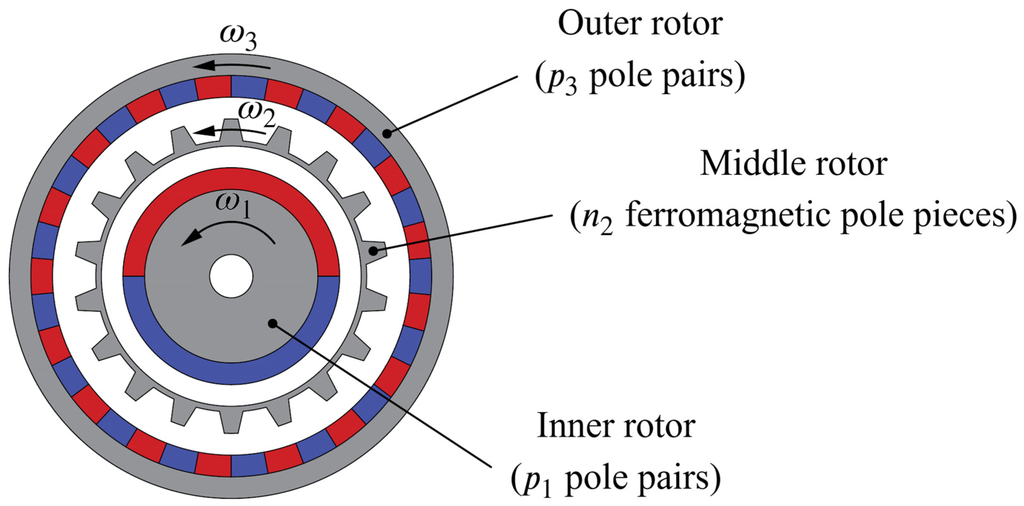
1.1. Essentials of Coaxial MGs

There are many different MG topologies (see [12] for a comprehensive overview of existing MG topologies). However, most of the ongoing research in this particular area is focused on coaxial MGs with radial flux orientation. This topology, which is first presented by Atallah and Howe in their milestone paper [6], is at this point considered preferable over other MG topologies due to its higher torque density [13] and a rather simple construction [14]. A coaxial MG (hereinafter to be referred to only as MG), whose cross-section is shown in Figure 1, consists of three major constructive parts, i.e., three rotors: an inner rotor with $p_1$ pole pairs, an outer rotor with $p_3$ pole pairs, and a middle rotor which is made of $n_2=p_1+p_3$ ferromagnetic pole pieces and placed in between the other two rotors. This middle rotor, also known as the modulator, is used to modulate the magnetic field produced by the permanent magnets (PMs) of the inner and outer rotor and is therefore essential for achieving torque transmission with a certain gear ratio (see [15] for how exactly the torque transmission in an MG is achieved).

In steady-state, the rotational speeds of the magnetic fields produced by the PMs of the inner and outer rotor are related to the electrical speed of the middle rotor through

$$p_1{\omega }_1+p_3{\omega }_3=n_2{\omega }_2,$$

(1)

where ${\omega }_1$, ${\omega }_2$ and ${\omega }_3$ are the mechanical speeds of the inner, middle and outer rotor, respectively. According to that, there are several possible operating modes of an MG depending on the speed of its rotors. However, the highest gear ratio can be achieved if the outer rotor is kept stationary (${\omega }_3=0$), whereby the inner rotor usually acts as the high-speed (HS) rotor and the middle rotor as the low-speed (LS) rotor. In this operating mode, which will be assumed throughout this paper, the gear ratio is given by

$$G_r=\frac{{\omega }_{hs}}{{\omega }_{ls}}=\frac{n_{ls}}{p_{hs}},$$

(2)

where ${\omega }_{hs}={\omega }_1$, ${\omega }_{ls}={\omega }_2$, $p_{hs}=p_1$ and $n_{ls}=n_2$ are introduced for the sake of clarity. Furthermore, assume that the HS rotor of the MG is driven by an electric motor and that a load is attached to the LS rotor. In that case, based on the conservation of power flow,

$$T_e{\omega }_{hs}-T_L{\omega }_{ls}=0$$

(3)

must hold, hence the steady-state relationship between the input (motor) torque $T_e$ and output (load) torque $T_L$ can be derived as

$$T_e=\frac{1}{G_r}{T}_L.$$

(4)

1.2. Control of Magnetic-Geared Drives: State-of-the-Art

A lot of research papers about MGs have been published until now. Yet, most of these papers deal with the design of MGs with emphasis put on improving their torque transfer capability and overall efficiency, whereas only a small portion of these papers deals with their control. From a control engineer’s point of view, an MG is not an “easy” system to deal with because of its low stiffness (e.g., a stiffness more than five times lower than that of a classic elastic coupling was reported in [8]) which is, in addition, not constant but varies (in a nonlinear way) with the load. However, this should not justify the significant lack of papers dealing with the control of magnetic-geared drives, especially since high-performance control is nowadays a prerequisite in many industrial applications.

With the exception of those in [16,17] which seem promising, but lack of a complete experimental verification, until now all presented control systems for magnetic-geared drives are based on well-known linear control techniques that have proven to be efficient and robust. As known to us, the problem of controlling magnetic-geared drives was first addressed in [18]. In that paper, a proportional-integral-derivative (PID) controller was used to control the speed of a magnetic-geared drive. Although it is not clear which of the two rotors was controlled, the oscillatory speed response has shown that the PID controller could not deal with the low stiffness of the drive, leading to the conclusion that either more attention should be given to the tuning of the controller or a different control approach should be used. In order to mitigate the oscillatory behaviour of the magnetic-geared drive, an optimally tuned proportional-integral (PI) controller was used in [19] to control the speed of its HS rotor. Assuming a linear instead of a nonlinear torque transfer characteristic, the authors first derived the transfer function of the closed-loop system, after which they determined the optimal gains of the controller (for the desired bandwidth) by comparing the coefficients of the characteristic polynomial with those of an ITAE (integral of the time weighted absolute error) polynomial of the same order. Experimental results have shown that the oscillations arising from the low stiffness of the MG can be sufficiently damped even with a simple PI controller, provided that the controller is optimally tuned. Moreover, the control system from [19] was further improved in [20] where a prefilter was introduced in the reference signal path, resulting in some kind of a two-degree-of-freedom (2DOF) controller. The prefilter was used to shape the reference signal in order to reduce the overshoot in the speed response which is a consequence of the closed-loop zeros. A similar approach can be found in [21] where a fractional-order PID controller was used to control the speed of the HS rotor. The controller gains, as well as the order of the controller’s integral and derivative term, were obtained using an open-source optimization package with the aim of minimizing the ITAE for a given step change in speed reference. An example of a more advanced linear control system can be found in [22,23,24,25]. In these papers, the speed control of the LS rotor is achieved with a state feedback controller that was designed based on the state space description of the linearized model of the MG. The state feedback controller was optimally tuned using a genetic algorithm with the objective of minimizing the ITAE for a given step change in speed reference. The performance of such a controller was compared to that of a PI controller. Experimental results have shown that fast and critically damped responses can be obtained while using a state feedback controller. The state space model of the MG was also used in [26] to design a state feedback-based speed controller within a model predictive control (MPC) framework. A nice feature of a model predictive controller is its ability to calculate, within a predefined time horizon, a sequence of optimal control inputs that are subject to a set of predefined constraints and will be applied over the next time horizon. However, the model predictive controller is in essence a quadratic programming approach for calculating optimal control inputs, hence its real-time implementation comes with high computational burden which often cannot be met by low-cost microcontrollers. In order to reduce the required computational effort, the authors of [26] used an explicit approach in which the optimal control inputs were calculated offline by dividing the state space into polyhedral regions defined by constraints imposed on the input torque and the torque transmitted from the HS to the LS side. The model predictive controller is thus implemented by means of a look-up-table which assigns an optimal control input to a particular set of state values. However, even with this, the control had to be executed every 10 milliseconds which may limit its application to drives that do not require fast dynamics. Nonetheless, a comparison with an optimally tuned PI controller has shown that a model predictive controller can reduce the possibility of entering a pole-slipping regime when high load is applied.

Apart from [16,17], the position control of magnetic-geared drives has only been addressed in [27]. The control system presented in that paper, which is actually the only position control system for magnetic-geared drives that went through a complete experimental evaluation (note that [16] considers only operation in no load, while [17] presents only simulation results), is based on a pseudo-derivative feedback (PDF) controller—a modified structure of a proportional-derivative (PD) controller in which the derivative term acts on the feedback instead on the error signal [28]. The optimal gains of the controller (in sense of ITAE) were calculated according to the tuning methodology presented in [29]. The experimental results confirmed that the torsional oscillations in the position of the magnetic-geared drive can be entirely suppressed by using a simple but optimally tuned controller. However, due to the lack of an integral term in the controller’s structure, a large steady-state error occurred after an external load torque was applied. Instead of enhancing the controller with an integral term, which would result in a PID-like structure, the authors used the load torque estimate as a feedforward signal to eliminate the steady-state error. Although effective and simple in structure, the position control system presented in [27] has a major drawback. As stated in [29], from which the design methodology was adopted, the optimal behaviour of the controller is guaranteed only if the inertias of the HS and LS rotor are approximately equal and the ratio between the closed-loop bandwidth and the drive’s anti-resonant frequency is 0.88. These requirements therefore considerably limit the application range of the presented control system.

1.3. Contribution and Overview of the Paper

Two main conclusions emerge from the brief overview of papers dealing with the control of magnetic-geared drives:

• Most of the research in this field has been focusing on speed rather than position control. The latter is, however, often used, especially in servo systems such as industrial robotic manipulators and computer numerically controlled (CNC) machine tools for which high-precision positioning is of great importance.
• Magnetic-geared drives are weakly damped systems in which fast torque actuation can easily excite torsional oscillations on both rotors. Therefore, control systems for magnetic-geared drives should be carefully designed in order to suppress those oscillations and ensure their high-performance dynamic behaviour.

Built upon these conclusions, this paper seeks to fill the gap in the existing literature on position control of magnetic-geared drives by presenting a novel observer-based position control system for a magnetic-geared servo drive. We truly believe that the design methodology explained in a step-by-step way, followed by from top to bottom described experiments, will be of use for any control engineer entering the field of magnetic-geared drives, whether he or she is involved in basic or applied research. On top of that, we believe that the work presented in this paper will make a small step toward the commercialization of magnetic-geared drives.

The position control system presented in this paper is based on two well established control strategies—field-oriented control (FOC) and state feedback control. The former is used to achieve effective torque control of a permanent magnet synchronous motor (PMSM) which is considered as an actuator that drives the HS rotor, whereas the latter is used to control the position of the LS rotor. The key difference between the control system presented in this paper and that presented in [27] (which is so far the only position control system for magnetic-geared drives that went through a complete experimental evaluation) is in the type of controller used to control the position of the LS rotor. In contrast to that of [27] which is based on a composite controller, the cornerstone of the control system presented in this paper is the state feedback controller. A state feedback controller offers more freedom when it comes to placing the poles of the closed-loop system than classic PI(D) controllers and their modifications, which is why it can be considered as an effective tool for suppressing the torsional modes of drive systems with flexible transmission like those incorporating MGs. Moreover, unlike the controller presented in [27] whose bandwidth is limited by the anti-resonant frequency of the drive, the bandwidth of the state feedback-based position controller used in this paper is limited only by the actuator dynamics. Even though the state feedback-based position controller requires all mechanical states to be known, it is possible to reduce the number of sensors required for its implementation by using a state observer. Therefore, a reduced-order extended state observer (ESO) is used in this paper to estimate the position and speed of the LS rotor which are assumed not available for measurement.

The rest of the paper is organized as follows. The modeling of the PMSM and the MG is revisited in Section 2. The design of the observer-based position control system is covered in Section 3. The experimental results are given and discussed in Section 4. The robustness of the presented control system against uncertainties in the inertia of the LS rotor is analyzed in Section 5. Finally, conclusions are made in Section 6.

2. Mathematical Model of a Magnetic-Geared PMSM

2.1. Mathematical Model of a PMSM

The design of control systems for AC machines is usually based on a dq model (see [30] for an introduction to high-performance control of AC machines). According to [31], the stator voltage equations of a PMSM can be written as:

$$u_{sd}=R_s{i}_{sd}+L_{sd}\frac{d{i}_{sd}}{dt}-p_m{\omega }_{hs}{L}_{sq}{i}_{sq}$$

(5)

$$u_{sq}=R_s{i}_{sq}+L_{sq}\frac{d{i}_{sq}}{dt}+p_m{\omega }_{hs}\left(L_{sd}{i}_{sd}+{\Psi }_{PM}\right),$$

(6)

where $u_{sd}$ and $u_{sq}$ are the stator voltage components, $i_{sd}$ and $i_{sq}$ are the stator current components, ${\omega }_{hs}$ is the speed of the motor that corresponds to the speed of the HS rotor, $R_s$ is the stator resistance, $L_{sd}$ and $L_{sq}$ are inductances in the d- and q-axis, respectively, $p_m$ is the pole pair number of the motor, and ${\Psi }_{PM}$ is the constant flux produced by the permanent magnets. Furthermore, the electrical torque produced in a PMSM is given by:

$$T_e=\frac{3}{2}{p}_m\left[{\Psi }_{PM}{i}_{sq}+\left(L_{sd}-L_{sq}\right)i_{sd}{i}_{sq}\right].$$

(7)

2.2. Mathematical Model of an MG

2.2.1. Nonlinear Model of an MG

An MG can be modeled as a mechanical system consisting of two rotating masses, representing the HS and LS rotor, which are separated by two ideal gearboxes and a spring with a nonlinear torque transfer characteristic, as shown in Figure 2.

Based on Figure 2, the equations of motion of the HS and LS rotor can be written as:

$$J_{hs}\frac{d{\omega }_{hs}}{dt}=T_e-b_{hs}{\omega }_{hs}-\frac{1}{G_r}{T}_{mg}$$

(8)

$$J_{ls}\frac{d{\omega }_{ls}}{dt}=T_{mg}-b_{ls}{\omega }_{ls}-T_L,$$

(9)

where $J_{hs}$ and $b_{hs}$ are the inertia and viscous friction coefficient of the HS rotor, $J_{ls}$ and $b_{ls}$ are the inertia and viscous friction coefficient of the LS rotor, and

$$T_{mg}=T_{max}\sin {\theta }_T$$

(10)

is the torque that is transmitted from the HS to the LS rotor. As seen, the transmitted torque depends on the so-called torque angle

$${\theta }_T=p_{hs}{\theta }_{hs}-n_{ls}{\theta }_{ls}$$

(11)

which represents the electrical displacement between the HS and LS rotor. The stable operating region of an MG is defined for torque angles between −90° and 90°, hence if the absolute value of the torque angle exceeds 90°, which corresponds to the maximum output torque $T_{max}$, the torque transmission will be lost.

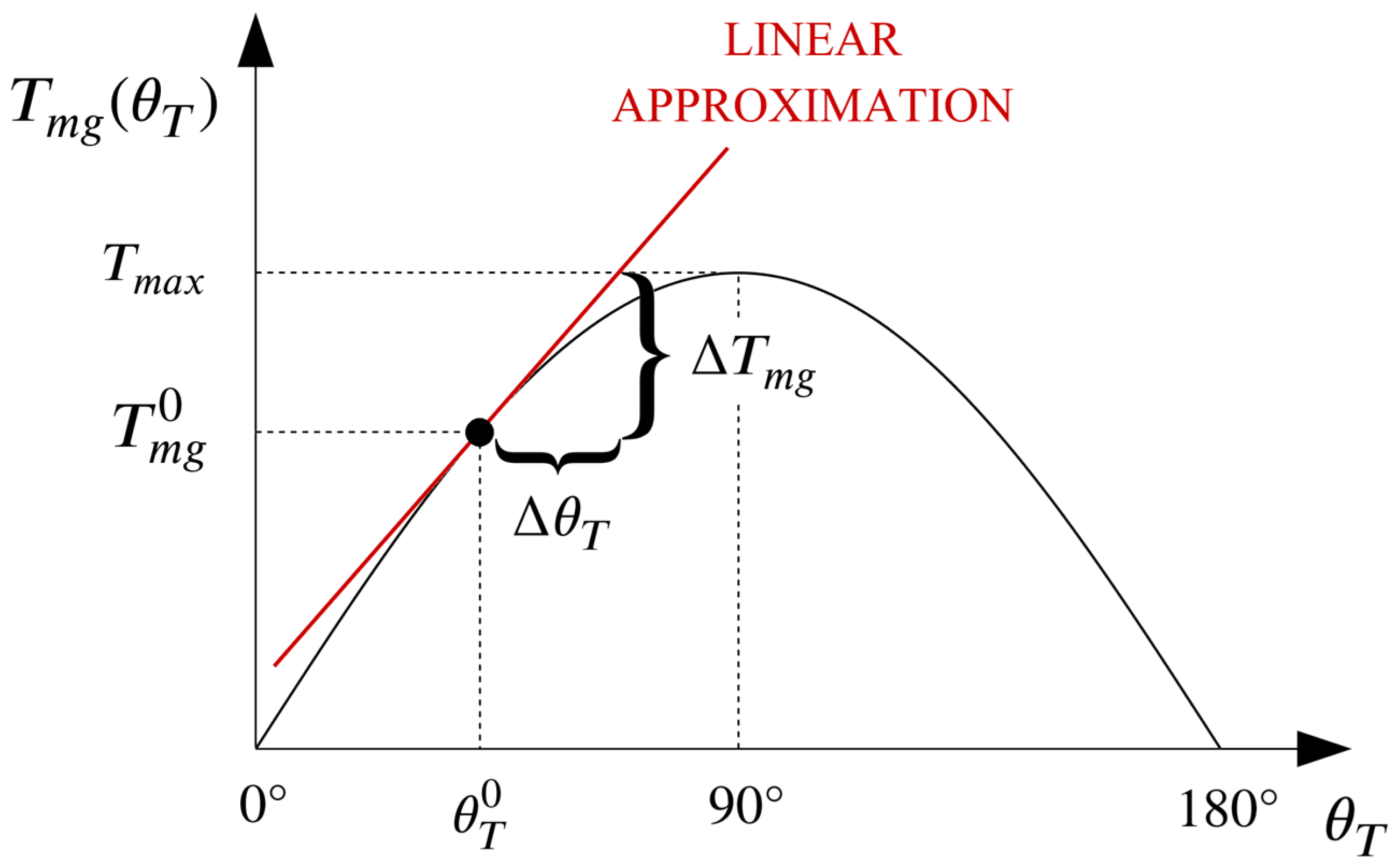
2.2.2. Linearized Model of an MG

In order to design a control system for a magnetic-geared drive using linear control techniques, a linear approximation of its nonlinear model has to be derived by linearizing the torque transfer characteristic around a fixed point, as show in Figure 3.

For the sake of simplicity, the no load point, which corresponds to a torque angle value of 0°, is chosen as the point around which the torque transfer characteristic will be linearized. As a result of that, Equation (10) can be rewritten as

$$T_{mg}=K_s{\theta }_T=K_s\left(p_{hs}{\theta }_{hs}-n_{ls}{\theta }_{ls}\right),$$

(12)

where

$$K_s={\left.\frac{\partial T_{mg}}{\partial {\theta }_T}\right|}_{{\theta }_T=0°}$$

is the linearized stiffness constant (in N·m/rad). Using (12), Equations (8) and (9) can be rewritten as

$$J_{hs}\frac{d{\omega }_{hs}}{dt}=T_e-b_{hs}{\omega }_{hs}-\frac{K_s}{G_r}\left(p_{hs}{\theta }_{hs}-n_{ls}{\theta }_{ls}\right)$$

(13)

$$J_{ls}\frac{d{\omega }_{ls}}{dt}=K_s\left(p_{hs}{\theta }_{hs}-n_{ls}{\theta }_{ls}\right)-b_{ls}{\omega }_{ls}-T_L,$$

(14)

whereby the relationship between the speeds and positions is given by

$$\frac{d{\theta }_{hs}}{dt}={\omega }_{hs}$$

(15)

$$\frac{d{\theta }_{ls}}{dt}={\omega }_{ls}.$$

(16)

Based on the linearized state equations of the MG, the transfer function between the input torque and the HS rotor position can be derived as

$$\frac{{\theta }_{hs}\left(s\right)}{T_e\left(s\right)}=\frac{p_{hs}}{J_{hs}}\frac{s^2+\frac{b_{ls}}{J_{ls}}s+\frac{n_{ls}{K}_s}{J_{ls}}}{s^4+\frac{J_{hs}{b}_{ls}+b_{hs}{J}_{ls}}{J_{hs}{J}_{ls}}{s}^3+\frac{K_s\left(n_{ls}{J}_{hs}+G_r^{-1}{p}_{hs}{J}_{ls}\right)+b_{hs}{b}_{ls}}{J_{hs}{J}_{ls}}{s}^2+\frac{K_s\left(n_{ls}{b}_{hs}+G_r^{-1}{p}_{hs}{b}_{ls}\right)}{J_{hs}{J}_{ls}}s},$$

(17)

whereas the transfer function between the input torque and the LS rotor position can be derived as

$$\frac{{\theta }_{ls}\left(s\right)}{T_e\left(s\right)}=\frac{p_{hs}}{J_{hs}}\frac{\frac{K_s}{J_{ls}}}{s^4+\frac{J_{hs}{b}_{ls}+b_{hs}{J}_{ls}}{J_{hs}{J}_{ls}}{s}^3+\frac{K_s\left(n_{ls}{J}_{hs}+G_r^{-1}{p}_{hs}{J}_{ls}\right)+b_{hs}{b}_{ls}}{J_{hs}{J}_{ls}}{s}^2+\frac{K_s\left(n_{ls}{b}_{hs}+G_r^{-1}{p}_{hs}{b}_{ls}\right)}{J_{hs}{J}_{ls}}s}.$$

(18)

The resonant nature of an MG can be seen from its common frequency response given in Figure 4, whereby its resonant ${\omega }_n$ and anti-resonant frequency ${\omega }_a$ can be easily estimated (by neglecting friction) from (17) and (18) as

$${\omega }_n=\sqrt{\frac{K_s}{G_r}\frac{G_r{n}_{ls}{J}_{hs}+p_{hs}{J}_{ls}}{J_{hs}{J}_{ls}}}, {\omega }_a=\sqrt{\frac{n_{ls}{K}_s}{J_{ls}}}.$$

Therefore, control systems for magnetic-geared drives should be carefully designed in order to suppress the oscillatory behaviour that arises from their resonant nature.

3. Observer-Based Position Control System

The main objective of this paper is to provide a design methodology for an observer-based position control system for a magnetic-geared servo drive. The developed position control system consists of two nested control loops. The inner control loop is used to achieve effective torque control of the PMSM which is considered as an actuator that provides the input torque for the MG. The outer control loop, which is based on an integral state feedback controller, is used for controlling the position of the LS rotor of the drive. Since it is assumed that no measurements are available on the LS rotor, the speed and position of the LS rotor, which are required to implement the state feedback controller, are estimated using a reduced-order ESO.

The schematic of the developed control system is shown in Figure 5. As seen, the input to the control system is the reference position of the LS rotor ${\theta }_{ls}^{\star }$ which is compared with the estimated position of the LS rotor ${\widehat{\theta }}_{ls}$ in order to calculate the position error. The position error is the input signal to the state feedback controller which is enhanced with an integral term and a simple anti-windup scheme. The integral term was introduced to ensure offset-free positioning and disturbance rejection.

The output of the state feedback controller represents the motor torque reference $T_e^{\star }$ which is the input to the inner control loop. The inner control loop is designed using the FOC principle, hence the q-axis stator current component is used for producing torque while the d-axis stator current component is kept zero in order to achieve maximum torque per ampere (in case where $L_{sd}\approx L_{sq}$). The reference for the q-axis stator current component $i_{sq}^{\star }$ is obtained by dividing the torque reference with the torque constant of the motor which is defined as

$$c_e=\frac{3}{2}{p}_m{\Psi }_{PM}.$$

(19)

Two PI controllers, whose transfer function is

$$G_{PI}\left(s\right)=K_P+\frac{K_I}{s},$$

(20)

are used to control the currents (one for each stator current component). The controller gains are chosen according to the internal model-based tuning scheme presented in [32] as

$$K_{Px}={\omega }_c{L}_{sx}$$

(21)

$$K_{Ix}={\omega }_c{R}_s,$$

(22)

where ${\omega }_c$ is the desired bandwidth of the current control loop (note that the x in the index stands for d or q). With these gains, the dynamics of each current control loop become equal to that of a first-order lag, i.e.,

$$\frac{i_{sx}\left(s\right)}{i_{sx}^{\star }\left(s\right)}=\frac{{\omega }_c}{s+{\omega }_c}.$$

(23)

Moreover, two feedforward signals, namely $∆u_{sd}=-p_m{\omega }_{hs}{L}_{sq}{i}_{sq}$ and $∆u_{sq}=p_m{\omega }_{hs}\left(L_{sd}{i}_{sd}+{\Psi }_{PM}\right)$, are added to the outputs of the current controllers (prior to the change of coordinates) in order to cancel the cross-coupling effect between the d- and q-axis. The schematic of the inner (torque) control loop is shown in Figure 6.

3.1. Design of the State Feedback Position Controller

If the inner control loop is fast enough in sense that the torque produced by the PMSM is approximately equal to its reference ($T_e\approx T_e^{\star }$), it is acceptable to simplify the design of the state feedback position controller by neglecting the electrical dynamics of the motor [33,34,35]. Therefore, the state feedback controller can be designed based on the state-space model of the MG given by

$$\frac{d}{dt}\mathbf{x}=\mathbf{A}\mathbf{x}+\mathbf{B}u,$$

(24)

where $\mathbf{x}={\left[\begin{array}{cccc}{\omega }_{hs}& {\theta }_{hs}& {\omega }_{ls}& {\theta }_{ls}\end{array}\right]}^{\mathrm{T}}$ is the state vector, $u=T_e$ is the control input, and

$$\mathbf{A}=\left[\begin{array}{cccc}-\frac{b_{hs}}{J_{hs}}& -\frac{p_{hs}{K}_s}{G_r{J}_{hs}}& 0& \frac{n_{ls}{K}_s}{G_r{J}_{hs}}\\ 1& 0& 0& 0\\ 0& \frac{p_{hs}{K}_s}{J_{ls}}& -\frac{b_{ls}}{J_{ls}}& -\frac{n_{ls}{K}_s}{J_{ls}}\\ 0& 0& 1& 0\end{array}\right], \mathbf{B}=\left[\begin{array}{c}\frac{1}{J_{hs}}\\ 0\\ 0\\ 0\end{array}\right]$$

are the state matrix and input vector, respectively.

Since $\mathbf{A}$ and $\mathbf{B}$ form a controllable pair, the system can be stabilized [36]. However, in order to ensure reference tracking, the system is augmented by introducing a new state variable which is defined as the integral of the tracking error:

$$e={\int }_0^{\infty }\left({\theta }_{ls}^{\star }-{\theta }_{ls}\right)dt.$$

(25)

The augmented system can then be written in state-space form as

$$\frac{d}{dt}\left[\begin{array}{c}\mathbf{x}\\ e\end{array}\right]=\left[\begin{array}{cc}\mathbf{A}& {\mathbf{0}}^{\mathbf{4}\times \mathbf{1}}\\ -\mathbf{C}& 0\end{array}\right]\left[\begin{array}{c}\mathbf{x}\\ e\end{array}\right]+\left[\begin{array}{c}\mathbf{B}\\ 0\end{array}\right]u+\left[\begin{array}{c}{\mathbf{0}}^{\mathbf{4}\times \mathbf{1}}\\ 1\end{array}\right]{\theta }_{ls}^{\star },$$

(26)

where ${\mathbf{0}}^{\mathbf{4}\times \mathbf{1}}$ is an empty column vector and $\mathbf{C}=\left[\begin{array}{cccc}0& 0& 0& 1\end{array}\right]$. Furthermore, if the control input is chosen as

$$u=-k_1{\omega }_{hs}-k_2{\theta }_{hs}-k_3{\omega }_{ls}-k_4{\theta }_{ls}+k_I{\int }_0^{\infty }\left({\theta }_{ls}^{\star }-{\theta }_{ls}\right)dt=-{\mathbf{K}}_{\mathbf{P}}\mathbf{x}+k_{I}e,$$

(27)

the resulting closed-loop system can be written as

$$\frac{d}{dt}\left[\begin{array}{c}\mathbf{x}\\ e\end{array}\right]=\left[\begin{array}{cc}\mathbf{A}-\mathbf{B}{\mathbf{K}}_{\mathbf{P}}& \mathbf{B}{k}_I\\ -\mathbf{C}& 0\end{array}\right]\left[\begin{array}{c}\mathbf{x}\\ e\end{array}\right]+\left[\begin{array}{c}{\mathbf{0}}^{\mathbf{4}\times \mathbf{1}}\\ 1\end{array}\right]{\theta }_{ls}^{\star }.$$

(28)

Hence, if the state matrix of the resulting closed-loop system is made Hurwitz by a suitable choice of controller gains,

$$\underset{t\to \infty }{\lim }{\theta }_{ls}\left(t\right)={\theta }_{ls}^{\star }$$

is guaranteed, whereby the transient behaviour is determined by the location of the closed-loop poles. Indeed, if the closed-loop system is made stable, the steady-state values of the state variables can be, in case of a constant reference, calculated from (28) by setting all the time derivatives to zero. After some simple algebraic manipulation one can obtain

$$\left[\begin{array}{c}{\mathbf{x}}^{ss}\\ e^{ss}\end{array}\right]=-{\left[\begin{array}{cc}\mathbf{A}-\mathbf{B}{\mathbf{K}}_{\mathbf{P}}& \mathbf{B}{k}_I\\ -\mathbf{C}& 0\end{array}\right]}^{-1}\left[\begin{array}{c}{\mathbf{0}}^{\mathbf{4}\times \mathbf{1}}\\ 1\end{array}\right]{\theta }_{ls}^{\star }$$

(29)

which yields

$$\left[\begin{array}{c}{\mathbf{x}}^{ss}\\ e^{ss}\end{array}\right]=\left[\begin{array}{c}{\omega }_{hs}^{ss}\\ {\theta }_{hs}^{ss}\\ {\omega }_{ls}^{ss}\\ {\theta }_{ls}^{ss}\\ e^{ss}\end{array}\right]=\left[\begin{array}{c}0\\ G_r\\ 0\\ 1\\ \frac{G_r{k}_2+k_4}{k_I}\end{array}\right]{\theta }_{ls}^{\star }.$$

As seen, in steady-state the position of the LS rotor is equal to its reference, the position of the HS rotor is equal to the position of the LS rotor times the gear ratio, and the speeds are zero since the drive is held in a fixed position. Also, note that the state variable representing the integral of the tracking error has a constant steady-state value. Hence, as expected, the steady-state tracking error is zero.

Recall that the output of the state feedback controller is in fact the motor torque reference. Therefore, for safety reasons the output of the state feedback controller should be limited to the maximum permissible torque value by applying a saturation function as follows:

$$T_e^{\star }=\mathrm{s}\mathrm{a}\mathrm{t}\left(u\right)=\left\{\begin{array}{cc}\hfill u,& \left|u\right|\le T_{e,max}\hfill \\ T_{e,max}\mathrm{sgn}\left(u\right),\hfill & \left|u\right|>T_{e,max}\hfill \end{array}\right.$$

(30)

The difference between the actual and saturated output of the state feedback controller is fed into a simple anti-windup scheme based on back calculation (see Figure 5), as proposed in [35].

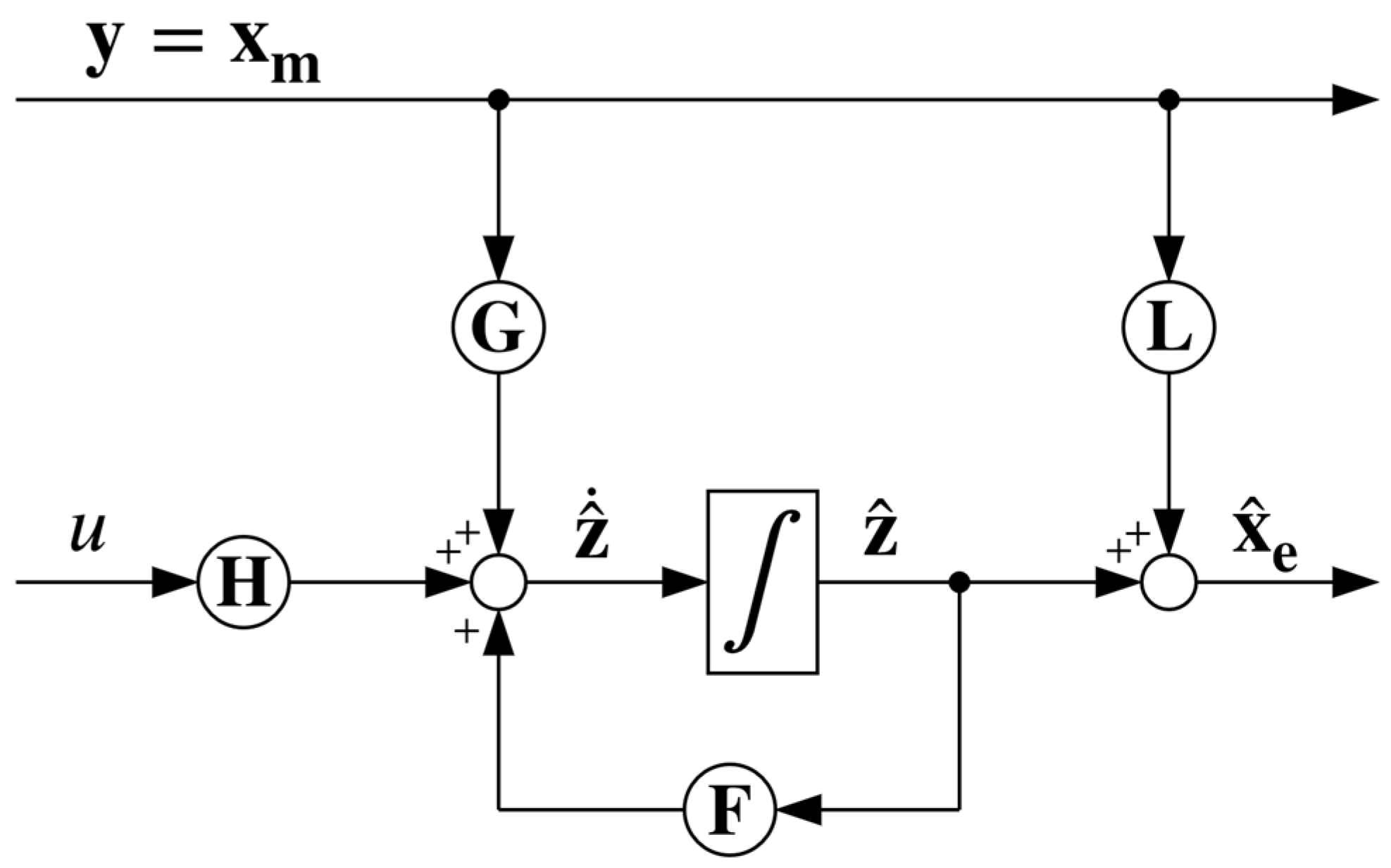
3.2. Design of the Reduced-Order ESO

Since the speed and position of the HS rotor are measured, a reduced-order observer is used instead of a full-order (Luenberger) observer in order to estimate only those states that are not measurable, namely the speed and position of the LS rotor. However, in order to prevent steady-state estimation error that may be caused by an unmodeled load torque, the state vector is extended with a new state that represents the unknown load torque which is assumed to be piecewise constant. Hence,

$$\frac{d{T}_L}{dt}=0$$

(31)

models the dynamics of the unknown load torque well enough.

By partitioning the extended state vector into states that are measured and states that have to be estimated, the state equation of the augmented system can be written as

$$\frac{d}{dt}\left[\begin{array}{c}{\mathbf{x}}_{\mathbf{m}}\\ {\mathbf{x}}_{\mathbf{e}}\end{array}\right]=\left[\begin{array}{cc}{\mathbf{A}}_{\mathbf{11}}& {\mathbf{A}}_{\mathbf{12}}\\ {\mathbf{A}}_{\mathbf{21}}& {\mathbf{A}}_{\mathbf{22}}\end{array}\right]\left[\begin{array}{c}{\mathbf{x}}_{\mathbf{m}}\\ {\mathbf{x}}_{\mathbf{e}}\end{array}\right]+\left[\begin{array}{c}{\mathbf{B}}_{\mathbf{1}}\\ {\mathbf{B}}_{\mathbf{2}}\end{array}\right]u,$$

(32)

where ${\mathbf{x}}_{\mathbf{m}}={\left[\begin{array}{cc}{\omega }_{hs}& {\theta }_{hs}\end{array}\right]}^{\mathrm{T}}$ is the part of states that is measured, ${\mathbf{x}}_{\mathbf{e}}={\left[\begin{array}{ccc}{\omega }_{ls}& {\theta }_{ls}& T_L\end{array}\right]}^{\mathrm{T}}$ is the part of states that has to be estimated, and ${\mathbf{A}}_{\mathbf{11}}$, ${\mathbf{A}}_{\mathbf{12}}$, ${\mathbf{A}}_{\mathbf{21}}$, ${\mathbf{A}}_{\mathbf{22}}$, ${\mathbf{B}}_{\mathbf{1}}$ and ${\mathbf{B}}_{\mathbf{2}}$ are given in Appendix A. The corresponding output equation is given by

$$\mathbf{y}={\mathbf{x}}_{\mathbf{m}}=\left[\begin{array}{cc}{\mathbf{I}}^{\mathbf{2}\times \mathbf{2}}& {\mathbf{0}}^{\mathbf{2}\times \mathbf{3}}\end{array}\right]\left[\begin{array}{c}{\mathbf{x}}_{\mathbf{m}}\\ {\mathbf{x}}_{\mathbf{e}}\end{array}\right],$$

(33)

where ${\mathbf{I}}^{\mathbf{2}\times \mathbf{2}}$ is a 2 × 2 identity matrix and ${\mathbf{0}}^{\mathbf{2}\times \mathbf{3}}$ is a 2 × 3 empty matrix.

The dynamics of the measured states are governed by

$$\frac{d}{dt}{\mathbf{x}}_{\mathbf{m}}={\mathbf{A}}_{\mathbf{11}}{\mathbf{x}}_{\mathbf{m}}+{\mathbf{A}}_{\mathbf{12}}{\mathbf{x}}_{\mathbf{e}}+{\mathbf{B}}_{\mathbf{1}}u,$$

(34)

which can be rearranged as

$$\frac{d}{dt}{\mathbf{x}}_{\mathbf{m}}-{\mathbf{A}}_{\mathbf{11}}{\mathbf{x}}_{\mathbf{m}}-{\mathbf{B}}_{\mathbf{1}}u={\mathbf{A}}_{\mathbf{12}}{\mathbf{x}}_{\mathbf{e}}$$

(35)

so that all terms related to the measured quantities are placed on one side of the equation and all terms related to the states that have to be estimated on the other. Moreover, the dynamics of the states that have to be estimated are governed by

$$\frac{d}{dt}{\mathbf{x}}_{\mathbf{e}}={\mathbf{A}}_{\mathbf{21}}{\mathbf{x}}_{\mathbf{m}}+{\mathbf{A}}_{\mathbf{22}}{\mathbf{x}}_{\mathbf{e}}+{\mathbf{B}}_{\mathbf{2}}u.$$

(36)

Following the procedure described in [37], an observer for (36) can be designed using (35) and (36) as

$$\frac{d}{dt}{\widehat{\mathbf{x}}}_{\mathbf{e}}=\underset{\mathrm{p}\mathrm{r}\mathrm{e}\mathrm{d}\mathrm{i}\mathrm{c}\mathrm{t}\mathrm{i}\mathrm{o}\mathrm{n}}{\underbrace{{\mathbf{A}}_{\mathbf{21}}{\mathbf{x}}_{\mathbf{m}}+{\mathbf{A}}_{\mathbf{22}}{\widehat{\mathbf{x}}}_{\mathbf{e}}+{\mathbf{B}}_{\mathbf{1}}u}}+\underset{\mathrm{c}\mathrm{o}\mathrm{r}\mathrm{r}\mathrm{e}\mathrm{c}\mathrm{t}\mathrm{i}\mathrm{o}\mathrm{n}}{\underbrace{\mathbf{L}\left(\frac{d}{dt}{\mathbf{x}}_{\mathbf{m}}-{\mathbf{A}}_{\mathbf{11}}{\mathbf{x}}_{\mathbf{m}}-{\mathbf{B}}_{\mathbf{1}}u-{\mathbf{A}}_{\mathbf{12}}{\widehat{\mathbf{x}}}_{\mathbf{e}}\right)}},$$

(37)

where ${\widehat{\mathbf{x}}}_{\mathbf{e}}={\left[\begin{array}{ccc}{\widehat{\omega }}_{ls}& {\widehat{\theta }}_{ls}& {\widehat{T}}_L\end{array}\right]}^{\mathrm{T}}$ is the vector of estimated states and $\mathbf{L}$ is the observer gain matrix. Notice that the reduced-order observer, just like that of a full-order, consists of a prediction term that mimics the observed system and a correction term that tends to make the difference between the actual system and its copy equal to zero.

The estimation error can be defined as

$${\tilde{\mathbf{x}}}_{\mathbf{e}}={\mathbf{x}}_{\mathbf{e}}-{\widehat{\mathbf{x}}}_{\mathbf{e}}.$$

(38)

Differentiating Equation (38) with respect to time yields

$$\frac{d}{dt}{\tilde{\mathbf{x}}}_{\mathbf{e}}=\frac{d}{dt}{\mathbf{x}}_{\mathbf{e}}-\frac{d}{dt}{\widehat{\mathbf{x}}}_{\mathbf{e}}.$$

(39)

Substituting the time derivatives on the right-hand side of (39) with (36) and (37) yields

$$\frac{d}{dt}{\tilde{\mathbf{x}}}_{\mathbf{e}}=\left({\mathbf{A}}_{\mathbf{22}}-\mathbf{L}{\mathbf{A}}_{\mathbf{12}}\right){\tilde{\mathbf{x}}}_{\mathbf{e}}.$$

(40)

Hence, if (40) is made stable by a suitable choice of observer gains,

$$\underset{t\to \infty }{\lim }‖{\tilde{\mathbf{x}}}_{\mathbf{e}}\left(t\right)‖=0$$

is guaranteed which implies that all estimated states converge to their true values as $t\to \infty$, with a convergence rate mainly determined by the location of the dominant pole of (40).

Note that the correction term in Equation (37) includes the derivative of the measured states which, from a practical standpoint, is not really desirable. However, by rearranging Equation (37) as

$$\frac{d}{dt}\left({\widehat{\mathbf{x}}}_{\mathbf{e}}-\mathbf{L}{\mathbf{x}}_{\mathbf{m}}\right)=\left({\mathbf{A}}_{\mathbf{22}}-\mathbf{L}{\mathbf{A}}_{\mathbf{12}}\right)\left({\widehat{\mathbf{x}}}_{\mathbf{e}}-\mathbf{L}{\mathbf{x}}_{\mathbf{m}}\right)+\left[\left({\mathbf{A}}_{\mathbf{22}}-{\mathbf{A}}_{\mathbf{11}}-\mathbf{L}{\mathbf{A}}_{\mathbf{12}}\right)\mathbf{L}+{\mathbf{A}}_{\mathbf{21}}\right]{\mathbf{x}}_{\mathbf{m}}+\left({\mathbf{B}}_{\mathbf{2}}-\mathbf{L}{\mathbf{B}}_{\mathbf{1}}\right)u,$$

(41)

it becomes clear that the differentiation of the measured signals, that can significantly amplify the noise contained in them, can be circumvented by applying the following change of coordinates:

$$\widehat{\mathbf{z}}={\widehat{\mathbf{x}}}_{\mathbf{e}}-\mathbf{L}{\mathbf{x}}_{\mathbf{m}}.$$

(42)

Hence, in the new coordinates, the observer is given by

$$\frac{d}{dt}\widehat{\mathbf{z}}=\mathbf{F}\widehat{\mathbf{z}}+\mathbf{G}\mathbf{y}+\mathbf{H}u,$$

(43)

where

$$\mathbf{F}={\mathbf{A}}_{\mathbf{22}}-\mathbf{L}{\mathbf{A}}_{\mathbf{12}}, \mathbf{G}=\left({\mathbf{A}}_{\mathbf{22}}-{\mathbf{A}}_{\mathbf{11}}-\mathbf{L}{\mathbf{A}}_{\mathbf{12}}\right)\mathbf{L}+{\mathbf{A}}_{\mathbf{21}},\mathbf{H}={\mathbf{B}}_{\mathbf{2}}-\mathbf{L}{\mathbf{B}}_{\mathbf{1}}.$$

Once the auxiliary states are estimated by integrating Equation (43), the state estimates in the original coordinates can be easily reconstructed as

$${\widehat{\mathbf{x}}}_{\mathbf{e}}=\widehat{\mathbf{z}}+\mathbf{L}{\mathbf{x}}_{\mathbf{m}}.$$

(44)

The schematic of the reduced-order ESO is shown in Figure 7.

3.3. Compensation of the Steady-State Estimation Error

The design of the ESO is also based on the linearized model of the mechanical subsystem. Therefore, at high loads, the difference between the actual torque transfer characteristic and its linear approximation can cause an error in the position estimate which of course affects the positioning accuracy. As proposed in [27], a correction signal defined as

$$∆{\widehat{\theta }}_{ls}=\frac{1}{n_2}\left[\frac{{\widehat{T}}_L}{K_s}-{\sin }^{-1}\left(\frac{{\widehat{T}}_L}{T_{max}}\right)\right]$$

(45)

is added to the estimated position of the LS rotor in order to eliminate the estimation error in steady-state. The correction signal is derived based on Equations (10) and (11) and the fact that the transmitted torque in steady-state is equal to the load torque.

4. Real-Time Implementation and Experimental Evaluation

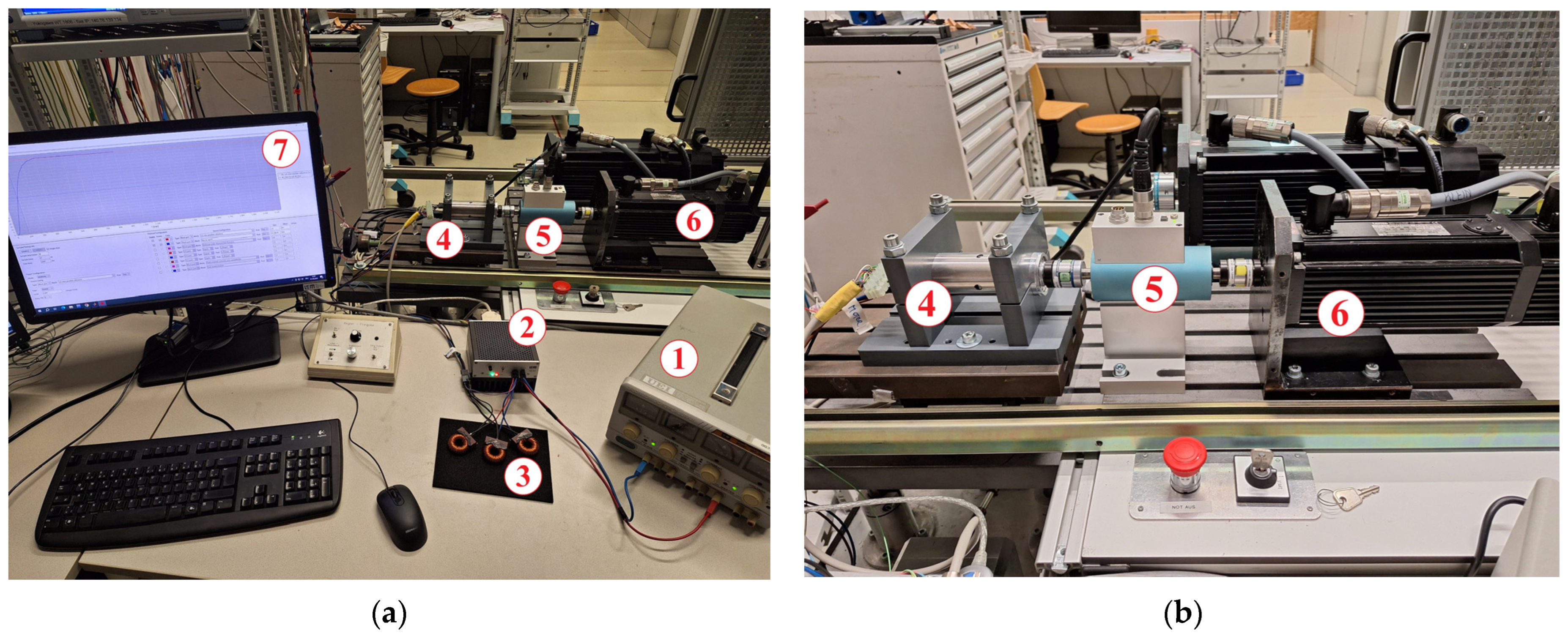
4.1. Experimental Setup

The experimental setup on which the developed control system was tested is shown in Figure 8. In essence, the experimental setup consisted of a laboratory power supply, an electronic control unit, a magnetic-geared PMSM and an induction machine which was controlled by a commercial drive and used as a load.

A prototype of a magnetic-geared motor with an 18:1 gear ratio that was designed by Jungmayr, Weidenholzer and Marth [38] was used in the experiments. In this prototype, the motor and the MG are placed next to each other within a common housing, sharing the same HS shaft. Such a side-by-side arrangement results with a low diameter-to-length ratio and a minimal number of bearings which are a significant source of losses at high speeds. The nominal data and parameters of the prototype are given in Appendix B, whereas far more details about its design and assembly can be found in [39,40].

The electronic control unit LCM-ECU-3HB-20A-48V was used, which acts as a three-phase inverter and a controller (see [41] for more details). The voltage for the DC link of the inverter was provided by a laboratory power supply. Furthermore, the motor has a toroidal stator winding with a very low inductance, hence three filter chokes (one for each phase) were placed between the inverter output and the motor terminals in order to reduce the current ripple, as well as the power losses related to that. The switching frequency of the inverter was set to 15 kHz. The control function is realized using a Texas Instruments’ TM4C123BE6PZ microcontroller which is based on a 32-bit floating point ARM Cortex-M4F microprocessor with a clock rate of 80 MHz (see [42] for detailed specifications). The developed control system was implemented using Code Composer Studio 8.3.1 together with X2C—a software that generates a C code for a graphically designed model of a control system, which makes it very comfortable for rapid prototyping purposes (see [43] for more details about X2C). The discrete-time integration was implemented using the forward Euler method and the control was executed every 66.7 microseconds.

The gains of the current controllers were calculated according to (21) and (22) for a desired bandwidth of 3000 rad/s and are given in

Table 1. Current controller gains.

Controller	$\mathbf{Proportional} \mathbf{Gain}, {\mathit{K}}_{\mathit{P}}$	$\mathbf{Integral} \mathbf{Gain}, {\mathit{K}}_{\mathit{I}}$
d-axis current controller	0.9559	405
q-axis current controller	0.9673	405

. Note that the expressions according to which the gains were calculated include motor parameters, namely stator resistance and inductance. Hence, these parameters had to be updated so that they also take into account the resistance and inductance of the filter chokes. The resistance and inductance of the filter chokes were measured using an RLC meter and are given in Appendix B. Although the main current limits were set to 13.15 A, a short-term current of 18.6 A was allowed. In a short time, a high current cannot overheat the motor. However, it can help to achieve fast positioning.

The gains of the state feedback controller were calculated using the place( ) command in Matlab (see [44] for a detailed explanation of the command) so that the closed-loop poles of the mechanical system are real and distinct. The gains of the state feedback controller are given in

Table 2. State feedback controller gains.

Gain	${\mathit{k}}_1$	${\mathit{k}}_2$	${\mathit{k}}_3$	${\mathit{k}}_4$	${\mathit{k}}_{\mathit{I}}$
Value	0.0049	0.0532	−0.0662	−0.3340	6.1471

.

The place( ) command was also used to calculate the gains of the observer. The bandwidth of the observer should be at least twice the bandwidth of the closed-loop system. However, although a wide bandwidth is desirable, high gains can in practice amplify high-frequency noise, hence a trade-off between the observer bandwidth and its noise attenuation properties has to be done. In our case, the poles of the observer are arranged in a Butterworth configuration, which for the same bandwidth results in lower gain values compared to an arrangement where all poles are placed on the real axis. The gains of the observer are given in

Table 3. Reduced-order ESO gains.

Gain	${\mathit{l}}_1$	${\mathit{l}}_2$	${\mathit{l}}_3$
Value	0.8656	0.0042	−0.0974

.

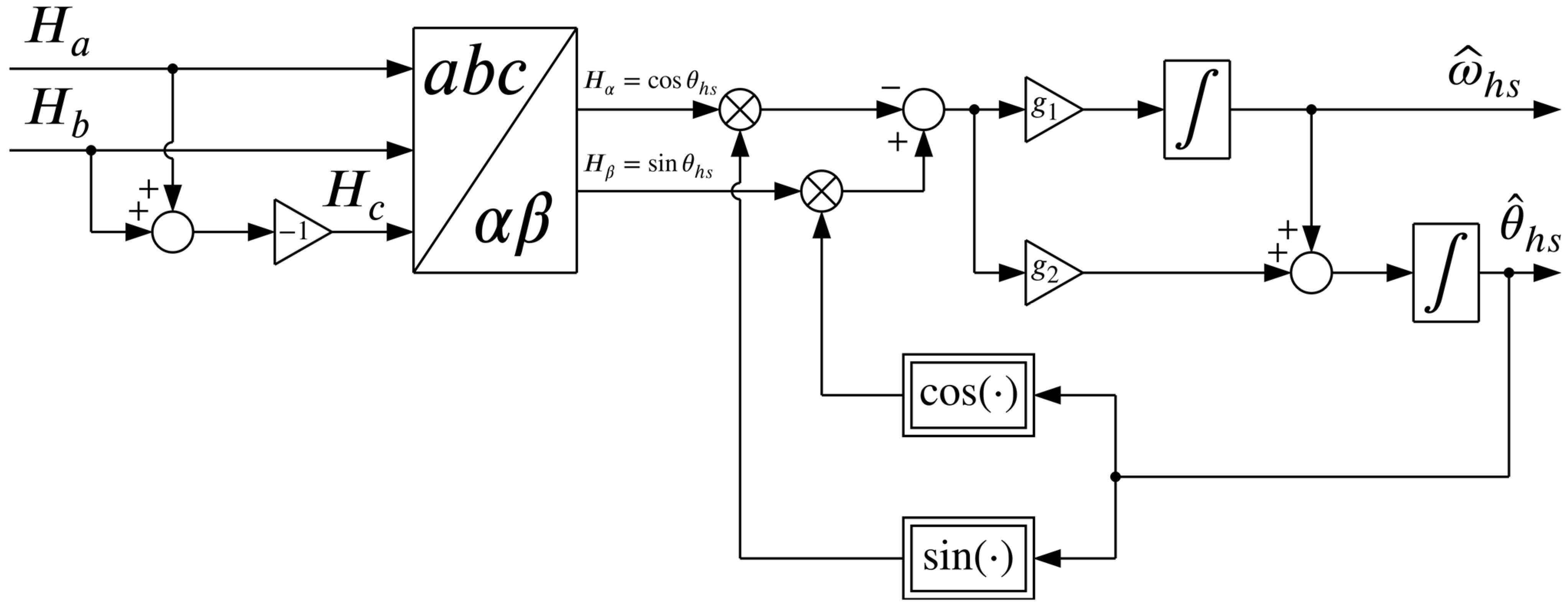
4.2. Measurement Processing

Recalling that the position and speed of the LS rotor are estimated using an observer, the real-time implementation of the developed control system only requires measurement of the position and speed of the HS rotor, as well as phase currents.

Two Hall sensors are placed on a printed circuit board inside the housing of the magnetic-geared motor with a spatial displacement of 120°. Each sensor provides a voltage signal equivalent to the measured magnetic field. These two voltage signals, let us denote them as $H_a$ and $H_b$, are sinusoidal functions of the HS rotor position (with a phase shift of 120°). Assuming that these signals are part of a symmetrical three-phase system for which

$$H_a\left(t\right)+H_b\left(t\right)+H_c\left(t\right)=0$$

(46)

holds for every time instant, a third signal $H_c$ can be easily reconstructed according to

$$H_c\left(t\right)=-H_a\left(t\right)-H_b\left(t\right).$$

(47)

By applying the Clarke transform to the three-phase signals $H_a$, $H_b$ and $H_c$, two mutually orthogonal signals $H_{\alpha }$ and $H_{\beta }$ can be obtained. The position of the HS rotor can then be determined using

$${\theta }_{hs}=\mathrm{atan}\left(\frac{H_{\beta }}{H_{\alpha }}\right).$$

(48)

However, despite their low cost, high reliability and small size, Hall sensors are often interfered by magnetic fields produced by the currents flowing through the surrounding phases. Together with some small mounting errors, this can affect the shape of the output signals and, as a consequence of that, deteriorate the calculated position signal. Moreover, a deteriorated position signal can cause imbalances in the phase currents (if FOC is employed), as well as a noisy speed signal if the speed is calculated by differentiating the position signal (even with additional low-pass filtering), as in most cases. High-quality measurement signals with a low noise content can only improve the performance of the control system. Therefore, a model-free observer, similar to that of [45], was used to reconstruct (estimate) the position and speed from the output signals of the Hall sensors. The dynamics of the observer are governed by a set of two differential equations that can be written in state-space form as

$$\frac{d}{dt}\left[\begin{array}{c}{\widehat{\theta }}_{hs}\\ {\widehat{\omega }}_{hs}\end{array}\right]=\left[\begin{array}{cc}0& 1\\ 0& 0\end{array}\right]\left[\begin{array}{c}{\widehat{\theta }}_{hs}\\ {\widehat{\omega }}_{hs}\end{array}\right]+\left[\begin{array}{c}{g}_1\\ g_2\end{array}\right]\epsilon$$

(49)

where ${\widehat{\theta }}_{hs}$ and ${\widehat{\omega }}_{hs}$ are the reconstructed position and speed of the HS rotor, respectively, $\epsilon$ is the error that drives the observer and is, just like in a phase-locked loop (PLL), defined using the small-angle approximation

$$\epsilon ={\theta }_{hs}-{\widehat{\theta }}_{hs}\approx \sin \left({\theta }_{hs}-{\widehat{\theta }}_{hs}\right)=\sin {\theta }_{hs}\cos {\widehat{\theta }}_{hs}-\cos {\theta }_{hs}\sin {\widehat{\theta }}_{hs},$$

(50)

and $g_1$ and $g_2$ are the observer gains. To ensure the convergence of the observer, its gains must be chosen so that the characteristic polynomial of the linearized error dynamics is Hurwitz stable. In our case, the observer gains are chosen by comparing the characteristic polynomial of the error dynamics with that of a stable second-order system having two real poles:

$$s^2+g_{2}s+g_1=s^2+2{\omega }_{o}s+{\omega }_o^2$$

(51)

It follows from (51) that the observer gains are $g_1={\omega }_o^2$ and $g_2=2{\omega }_o$, where ${\omega }_o$ can be considered as the bandwidth of the observer and is set to 200 rad/s. The schematic of the model-free observer is shown in Figure 9. Note that the per-unit scaling and offset compensation of the Hall sensor outputs, namely $H_a$ and $H_b$, are not drawn. The model-free observer is, like the rest of the control system, discretized using the forward Euler method.

The magnetic-geared motor and the induction machine were coupled via a torque sensor. The torque sensor also contains a high-resolution incremental encoder. Although the position and speed of the LS rotor are estimated using an observer, the position signal provided by the encoder was used for validation only. On the other hand, the torque signal was fed into and monitored (in value only) on a power analyzer since there were no more analog inputs available on the electronic control unit. Finally, it should be noted that the sampling of all measurements was synchronized with the pulse width modulation (PWM) of the inverter.

4.3. Static Measurements

Theoretically, the torque transfer characteristic of an MG is a sinusoidal function of its torque angle. However, in reality, the MG may not be perfectly manufactured. For example, if the modulator is not perfectly shaped or if it is not rigid enough, the torque transfer characteristic may not have a perfect sinusoidal shape. Therefore, static measurements were performed to assess the torque transfer characteristic of the used prototype. A better understanding of the prototype can be of help when its behaviour under the developed control system will have to be evaluated.

In order to measure the static torque transfer characteristic, the experimental setup was reconfigured as shown in Figure 10a. The induction machine was temporarily replaced with a lathe head that is equipped with a highly accurate rotation mechanism. The shaft of the torque sensor was inserted inside the jaws of the lathe head and locked-in together with the output shaft (LS rotor) of the magnetic-geared motor. Furthermore, a PID controller was used to hold the HS rotor in a fixed position, declared as 0°. With a fixed HS rotor, the lathe head was rotated in steps of approximately 0.56° which corresponds to 10° electrical (recall that the number of ferromagnetic pole pieces of the LS rotor is $n_{ls}=18$). For each step, the position and torque measured by the torque sensor were recorded and the torque transfer characteristic of the magnetic-geared motor was reconstructed by interpolating the data from each step (see Appendix C). The actual torque transfer characteristic with a peak value of 2.489 N·m is shown in Figure 10b. As expected, the measured torque increased with each step, as each step was actually an increase in the torque angle. However, as seen, the actual torque transfer characteristic does not have an ideal sinusoidal shape but is slightly flattened in some of its parts.

4.4. Experimental Evaluation of the Presented Position Control System

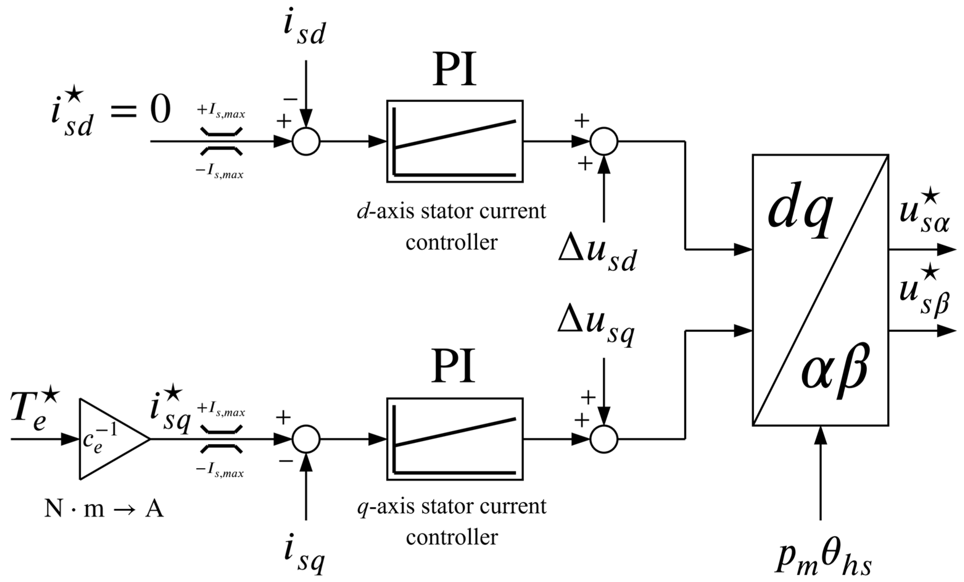
4.4.1. Experimental Results: Current Control

Once the static measurements were performed, the lathe head was replaced with the induction machine. The C code for the observer-based position control system was generated using X2C and uploaded on the microcontroller. In the case of nested control loops, it is usually recommended to first check if the inner current control loop works properly. The performance of each current controller was evaluated by applying a step change from 0 to 2 A in the current reference. The responses of the d- and q-axis stator current component for such a step change in reference are shown in Figure 11. As seen, the current responses are similar to that of a first-order lag component and the settling time is less than half of a millisecond.

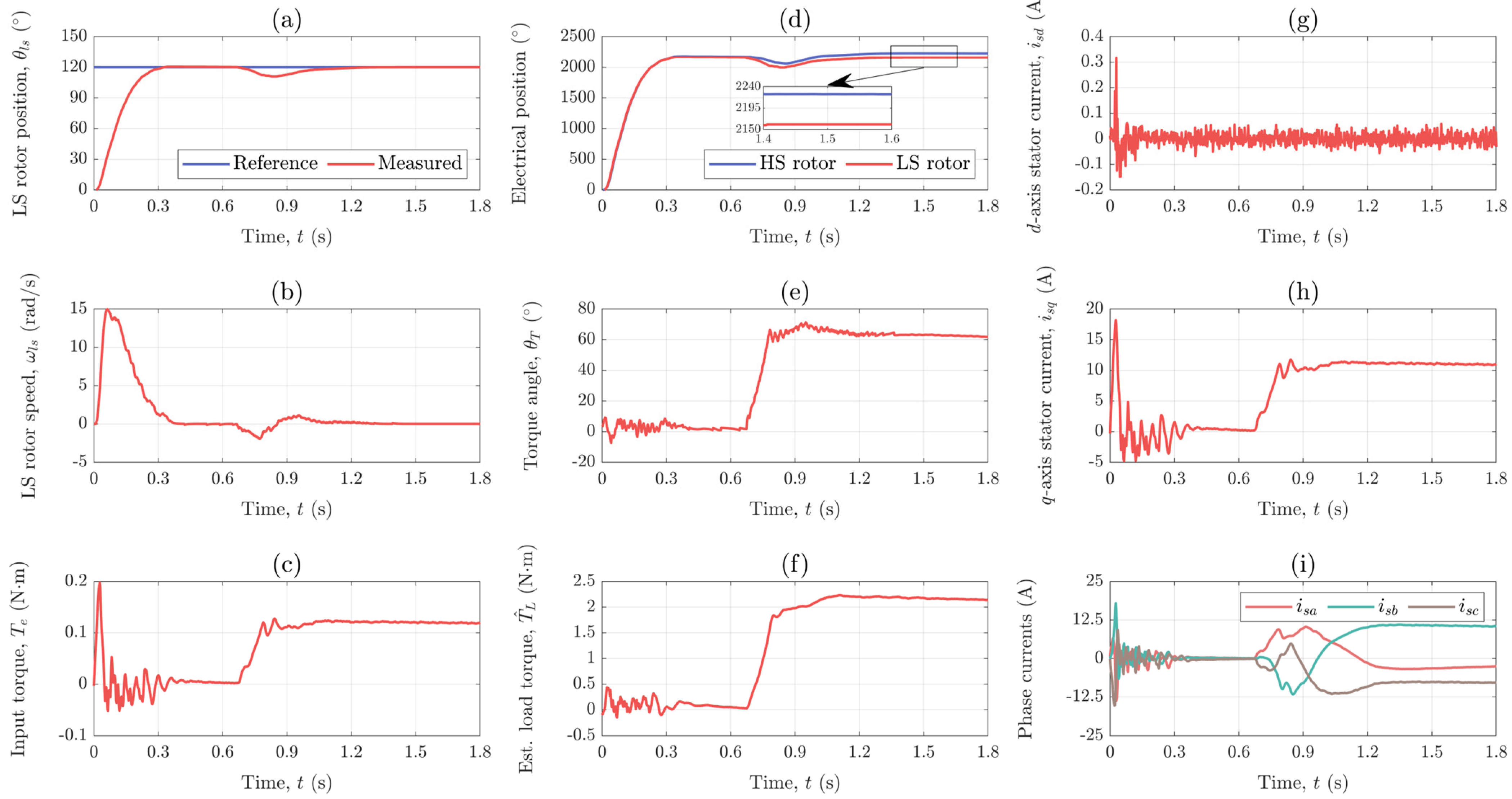
4.4.2. Experimental Results: Position Control (Scenario I)

The first scenario for which the developed control system was tested involves a step change of 120° in the reference for the position of the LS rotor that occurs at t = 0 s and a disturbance caused by applying a load torque equal to 80% of the MG’s maximum output torque at t = 0.7 s.

The position of the LS rotor is shown in Figure 12a, together with its reference. As seen, the position response is nicely overdamped and the reference position is reached within 0.3 s. Furthermore, once the load torque is applied, the position drops to approximately 110°, but successfully recovers to its reference value in less than 0.5 s.

Figure 12b shows the speed of the LS rotor that was calculated by differentiating the position signal provided by the encoder that is integrated within the torque sensor. The highest speed value, namely 15 rad/s (143 rpm) for the LS rotor and 284 rad/s (2713 rpm) for the HS rotor, is reached during positioning, whereas in steady-state the speed is zero. This is expected because the speed represents the rate of change in position.

The input torque of the MG, i.e., the electrical torque of the PMSM is calculated based on the measured currents and shown in Figure 12c. As seen, at t = 0 s the motor produces a torque of almost 0.2 N·m in order to bring the LS rotor in the desired position. Once the reference position is reached, the motor torque becomes almost equal to zero until t = 0.7 s when a load torque equal to 80% of the MG’s maximum output torque, which is about 1.991 N·m, is applied. The motor torque then increases to a value of 0.123 N·m which is, considering the gear ratio of the MG, about 0.012 N·m higher than expected. This might be due to some small cogging torque that is present in PM machines and MGs.

The electrical positions of the HS and LS rotor are shown in Figure 12d. From t = 0 s to t = 0.7 s, the drive is in no load and the HS and LS rotor are electrically aligned. As seen, the loading of the drive is followed by an electrical displacement between the two rotors which is necessary for the torque transmission. Since the controller holds the LS rotor in the desired position, the torque transmission is achieved by an increase in the position of the HS rotor. The electrical displacement between the HS and LS rotor, i.e., the torque angle is shown in Figure 12e. As seen, under a load of 1.991 N·m, the steady-state value of the torque angle is 62.80°. This is more or less in accordance with the data obtained from static measurements (see Appendix C) where an output torque of 2.03 N·m was measured for a torque angle of 60.10° which was manually set using the lathe head.

Figure 12f shows the load torque estimated using the reduced-order ESO. The steady-state value of the load torque estimate under load is 2.149 N·m, which is somewhat higher than the actual load torque of 1.991 N·m. This overestimation of the load torque could be caused by some uncertainties in model parameters such as the torque constant or the maximum output torque of the MG. However, since the observer actually estimates the total disturbance, it could also be that some cogging torque is taken into account by the load torque estimate.

The d- and q-axis stator current components are shown in Figure 12g and 12h, respectively. As seen, the d-axis stator current component is kept to zero, whereas the q-axis stator current component is used to produce the torque that drives the HS rotor, which is why its shape is same as that of the motor torque shown in Figure 12c. The motor phase currents are shown in Figure 12i. Since the motor is not running, the phase currents have a DC steady-state value.

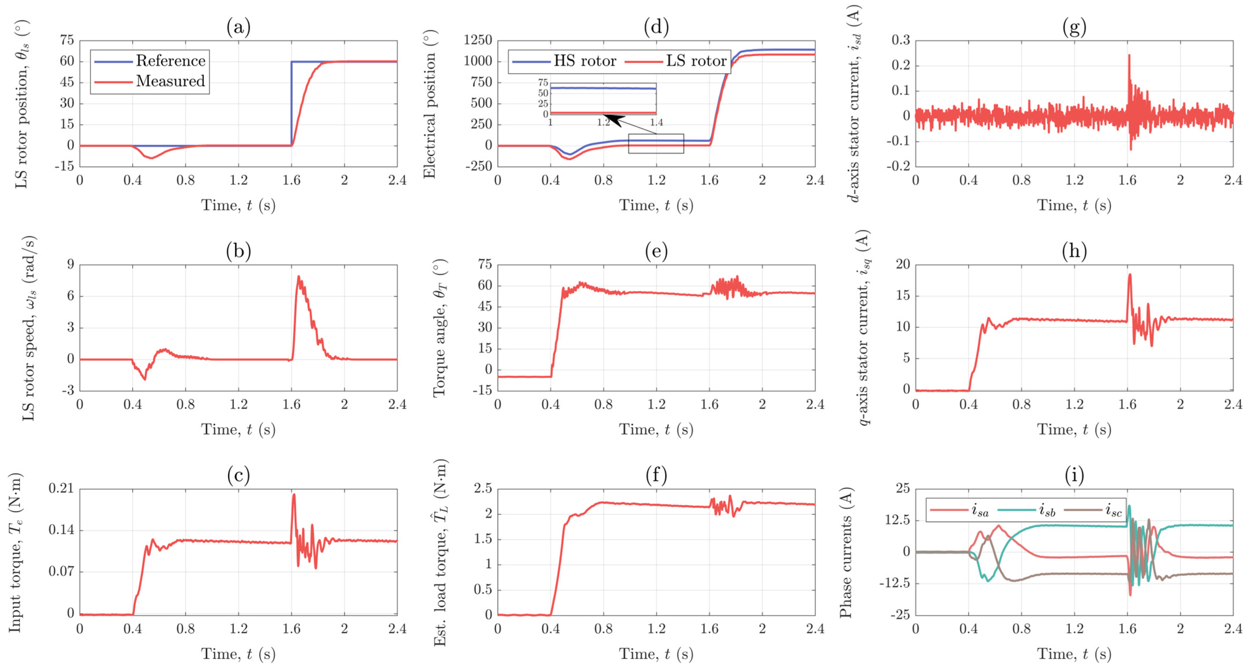
4.4.3. Experimental Results: Position Control (Scenario II)

The state feedback controller was designed based on a model that was linearized around the no load point, hence it was necessary to check whether the controller maintains its performance over the whole operating range or not by performing an additional experiment which included positioning under load. More precisely, the magnetic-geared drive was loaded with 80% of its maximum output torque at t = 0.4 s and a step change of 60° in the reference for the position of the LS rotor was applied at t = 1.6 s. In comparison to the previous experiment, a smaller step change was applied only to avoid hitting the current limits.

The reference and actual position of the LS rotor are shown in Figure 13a. As seen, the controller rejects the disturbance caused by the applied load torque within 0.5 s. Regarding the position response, it is nicely overdamped and the reference position is reached within 0.3 s, just like in the previous experiment in which the positioning was performed in no load.

The speed of the LS rotor is shown in Figure 13b. The highest speed value, namely 8 rad/s (76 rpm) for the LS rotor and 147 rad/s (1402 rpm) for the HS rotor, is reached during positioning. The highest speed is about two times lower than in the previous experiment. However, the previous experiment also included a two times larger step change in position reference.

Figure 13c shows the input torque of the MG provided by the PMSM. The motor torque is zero until t = 0.4 s when the drive is loaded with 80% of its maximum output torque, which is about 1.991 N·m. The motor torque then increases to 0.121 N·m which is, just like in the previous experiment, somewhat higher than expected considering the gear ratio. At t = 1.6 s, the motor torque rises to 0.2 N·m in order to bring the LS rotor in the desired position. Once the reference position is reached, the motor torque assumes again a value of 0.121 N·m.

The electrical positions of the HS and LS rotor are shown in Figure 13d. As seen, the HS and LS rotor are electrically aligned until t = 0.4 s when the position of the HS rotor is increased in order to enable the torque transmission between the two rotors. The electrical displacement between the HS and LS rotor, i.e., the torque angle is shown in Figure 13e. The steady-state value of the torque angle under load is 54.70°. However, since the torque angle before t = 0.4 s is −5°, the increase in the torque angle caused by the load is 59.70°, which is close to 62.80° obtained in the previous experiment. Although not significant, the difference between these two values can be explained by the fact that the position of the LS rotor was not the same in both experiments. This may also explain why the torque angle in this experiment is not exactly zero in no load.

The load torque estimate is shown in Figure 13f. The steady-state value of the load torque estimate under load is 2.148 N·m which is 0.157 N·m higher than the actual load torque. As said, the overestimation of the load torque could be caused by some uncertainties in model parameters or by some small unmodeled disturbances (e.g., cogging torque).

The d- and q-axis stator current components are shown in Figure 13g and 13h, respectively. As seen, the d-axis stator current component is kept to zero, whereas the q-axis stator current component is used to produce torque. The steady-state value of the torque producing stator current component under load is 11 A. Finally, the motor phase currents are shown in Figure 13i. As said, since the motor is being held in a fixed position, in steady-state the phase currents are DC quantities.

Since it is extremely difficult to create a simulation model that would take into account the actual torque transfer characteristic of the used prototype (at least without acquiring more data through static measurements) and thus be able to accurately predict all physical quantities shown in Figure 12 and Figure 13, a comparison between experimental and simulation results is not given. A simulation model in which the torque transfer characteristic is modeled as a sine function was used only for a preliminary evaluation of the developed control system and a rough assessment of its robustness against parametric uncertainties.

5. Simulation-Based Robustness Analysis

Since the observer-based position control system is designed assuming nominal system parameters, it is necessary to analyze its robustness against uncertainties in mechanical parameters (recall that the controller and observer are designed based on the state-space model of the mechanical subsystem of a magnetic-geared drive). The only mechanical parameters that is subject to variations is the inertia of the LS rotor whose value also depends on the attached load. In order to investigate the influence of uncertainties in the inertia of the LS rotor on the overall performance of the presented control system, a simulation model of the magnetic-geared PMSM and the observer-based position control system was built in Matlab/Simulink. A scenario in which a step change of 120° in the reference for the position of the LS rotor occurred at t = 0 s followed by a disturbance caused by applying a load torque equal to 80% of the MG’s maximum output torque at t = 0.7 s was simulated for different values of the LS rotor inertia. The gains of the controller and observer used in simulation were exactly the same as those used in the experiments. The simulation results shown in Figure 14 indicate that the presented control system is quite robust against uncertainties in the inertia of the LS rotor. More precisely, the position response does not deteriorate even for a 200% increase in inertia. Although a 400% increase in inertia leads to instability, we believe that this margin can be further increased (to a certain degree) by increasing the bandwidth of the observer.

6. Conclusions

A novel observer-based position control system for a magnetic-geared PMSM drive has been presented in this paper with the aim of filling the gap in the existing literature on position control of magnetic-geared drives and making a small step towards the commercialization of such drives. The presented control system consists of two nested control loops. The inner control loop ensures effective torque control of the PMSM which is considered as an actuator that drives the HS rotor. The outer control loop, on the other hand, is used to control the position of the LS rotor. The position control of the LS rotor is achieved with an integral state feedback controller, whereby a reduced-order ESO is used to estimate the position and speed of the LS rotor in order to reduce the number of sensors required for its implementation. Furthermore, the presented control system was implemented on a microcontroller and tested on an existing prototype with a gear ratio of 18:1. The experimental results showed that a desired position of 120° (or less) can be reached within 0.3 s and that disturbances caused by a load torque can be rejected in less than 0.5 s. Moreover, experiments that included positioning under load showed that the controller maintains its high performance over the whole operating range of the drive.

References

1. Nielsen, S.S.; Holm, R.K.; Rasmussen, P.O. Conveyor System With a Highly Integrated Permanent Magnet Gear and Motor. IEEE Trans. Ind. Appl. 2020, 56, 2550–2559. [Google Scholar] [CrossRef]
2. Frandsen, T.V.; Mathe, L.; Berg, N.I.; Holm, R.K.; Matzen, T.N.; Rasmussen, P.O.; Jensen, K.K. Motor Integrated Permanent Magnet Gear in a Battery Electrical Vehicle. IEEE Trans. Ind. Appl. 2015, 51, 1516–1525. [Google Scholar] [CrossRef]
3. Jian, L.; Chau, K.T.; Jiang, J.Z. A Magnetic-Geared Outer-Rotor Permanent-Magnet Brushless Machine for Wind Power Generation. IEEE Trans. Ind. Appl. 2009, 45, 954–962. [Google Scholar] [CrossRef]
4. Hazra, S.; Kamat, P.; Bhattacharya, S.; Ouyang, W.; Englebretson, S. Power Conversion With a Magnetically-Geared Permanent Magnet Generator for Low-Speed Wave Energy Conversion. IEEE Trans. Ind. Appl. 2020, 56, 5308–5318. [Google Scholar] [CrossRef]
5. Martin, T.B. Magnetic Transmission. U.S. Patent 3378710A, 16 April 1968. [Google Scholar]
6. Atallah, K.; Howe, D. A Novel High-Performance Magnetic Gear. IEEE Trans. Magn. 2001, 37, 2844–2846. [Google Scholar] [CrossRef]
7. Atallah, K.; Calverley, S.D.; Howe, D. Design, analysis and realization of a high-performance magnetic gear. IEE Proc.-Electr. Power Appl. 2004, 151, 135–143. [Google Scholar] [CrossRef]
8. Rasmussen, P.O.; Andersen, T.O.; Jørgensen, F.T.; Nielsen, O. Development of a High-Performance Magnetic Gear. IEEE Trans. Ind. Appl. 2005, 41, 764–770. [Google Scholar] [CrossRef]
9. Jungmayr, G.; Loeffler, J.; Winter, B.; Jeske, F.; Amrhein, W. Magnetic Gear: Radial Force, Cogging Torque, Skewing, and Optimization. IEEE Trans. Ind. Appl. 2016, 52, 3822–3830. [Google Scholar] [CrossRef]
10. Göbl, E.; Jungmayr, G.; Marth, E.; Amrhein, W. Optimization and Comparison of Coaxial Magnetic Gears With and Without Back Iron. IEEE Trans. Magn. 2018, 54, 1–4. [Google Scholar] [CrossRef]
11. Wong, H.Y.; Baninajar, H.; Dechant, B.W.; Southwick, P.; Bird, J.Z. Experimentally Testing a Halbach Rotor Coaxial Magnetic Gear With 279 Nm/L Torque Density. IEEE Trans. Energy Convers. 2023, 38, 507–518. [Google Scholar] [CrossRef]
12. Wang, Y.; Filippini, M.; Bianchi, N.; Alotto, P. A Review on Magnetic Gears: Topologies, Computational Models, and Design Aspects. IEEE Trans. Ind. Appl. 2019, 55, 4557–4566. [Google Scholar] [CrossRef]
13. Chen, Y.; Fu, W.N.; Ho, S.L.; Liu, H. A Quantitative Comparison Analysis of Radial-Flux, Transverse-Flux, and Axial-Flux Magnetic Gears. IEEE Trans. Magn. 2014, 50, 1–4. [Google Scholar] [CrossRef]
14. Gardner, M.C.; Johnson, M.; Toliyat, H. Comparison of Surface Mounted Permanent Magnet Axial and Radial Flux Coaxial Magnetic Gears. IEEE Trans. Energy Convers. 2018, 33, 2250–2259. [Google Scholar] [CrossRef]
15. Jian, L.; Deng, Z.; Shi, Y.; Wei, J.; Chan, C.C. The Mechanism How Coaxial Magnetic Gear Transmits Magnetic Torques Between Its Two Rotors: Detailed Analysis of Torque Distribution on Modulating Ring. IEEE/ASME Trans. Mechatron. 2019, 24, 763–773. [Google Scholar] [CrossRef]
16. Montague, R.; Bingham, C. Nonlinear Control of Magnetically-geared Drive-trains. Int. J. Autom. Comput. 2013, 10, 319–326. [Google Scholar] [CrossRef]
17. Verbanac, N.; Bulić, N.; Jungmayr, G.; Marth, E. Nonlinear Position Control of a Magnetic-Geared Servo Drive With Unknown Load. In Proceedings of the 2022 International Conference on Smart Systems and Technologies (SST), Osijek, Croatia, 19–20 October 2022; pp. 263–268. [Google Scholar] [CrossRef]
18. Montague, R.G.; Bingham, C.M.; Atallah, K. Magnetic gear overload detection and remedial strategies for servo-drive systems. In Proceedings of the 2010 International Symposium on Power Electronics, Electrical Drives, Automation and Motion (SPEEDAM), Pisa, Italy, 14–16 June 2010; pp. 523–528. [Google Scholar] [CrossRef]
19. Montague, R.; Bingham, C.; Atallah, K. Servo Control of Magnetic Gears. IEEE/ASME Trans. Mechatron. 2012, 17, 269–278. [Google Scholar] [CrossRef]
20. Liao, X.; Bingham, C.; Zolotas, A.; Zhang, Q.; Smith, T. Servo Control of Drive-Trains Incorporating Magnetic Couplings. IEEE Trans. Ind. Appl. 2022, 58, 3674–3684. [Google Scholar] [CrossRef]
21. Liao, X.; Bingham, C.; Smith, T. Speed Control of Magnetic Drive-Trains with Pole-Slipping Amelioration. Energies 2022, 15, 8148. [Google Scholar] [CrossRef]
22. Bouheraoua, M.; Wang, J.; Atallah, K. Design and implementation of an observer-based state feedback controller for a pseudo direct drive. IET Electr. Power Appl. 2013, 7, 643–653. [Google Scholar] [CrossRef]
23. Bouheraoua, M.; Wang, J.; Atallah, K. Speed Control for a Pseudo Direct Drive Permanent-Magnet Machine With One Position Sensor on Low-Speed Rotor. IEEE Trans. Ind. Appl. 2014, 50, 3825–3833. [Google Scholar] [CrossRef]
24. Bouheraoua, M.; Wang, J.; Atallah, K. Slip Recovery and Prevention in Pseudo Direct Drive Permanent-Magnet Machines. IEEE Trans. Ind. Appl. 2015, 51, 2291–2299. [Google Scholar] [CrossRef]
25. Bouheraoua, M.; Wang, J.; Atallah, K. Rotor Position Estimation of a Pseudo Direct-Drive PM Machine Using Extended Kalman Filter. IEEE Trans. Ind. Appl. 2017, 53, 1088–1095. [Google Scholar] [CrossRef]
26. Montague, R.G.; Bingham, C.; Atallah, K. Magnetic Gear Pole-Slip Prevention Using Explicit Model Predictive Control. IEEE/ASME Trans. Mechatron. 2012, 18, 1535–1543. [Google Scholar] [CrossRef]
27. Montague, R.G.; Bingham, C.M.; Atallah, K. Dual-observer-based position-servo control of a magnetic gear. IET Electr. Power Appl. 2011, 5, 708–714. [Google Scholar] [CrossRef]
28. Ohm, D.Y. Analysis of PID and PDF compensators for motion control systems. In Proceedings of the 1994 IEEE Industry Applications Society Annual Meeting, Denver, CO, USA, 2–6 October 1994; pp. 1923–1929. [Google Scholar] [CrossRef]
29. O’Sullivan, T.M.; Bingham, C.M.; Schofield, N. High-Performance Control of Dual-Inertia Servo-Drive Systems Using Low-Cost Integrated SAW Torque Transducers. IEEE Trans. Ind. Electron. 2006, 53, 1226–1237. [Google Scholar] [CrossRef]
30. Chiasson, J. Modeling and High-Performance Control of Electric Machines, 1st ed.; John Wiley & Sons, Inc.: Hoboken, NJ, USA, 2005. [Google Scholar]
31. Bodson, M.; Chiasson, J.N.; Novotnak, R.T.; Rekowski, R.B. High-Performance Nonlinear Feedback Control of a Permanent Magnet Stepper Motor. IEEE Trans. Control. Syst. Technol. 1993, 1, 5–14. [Google Scholar] [CrossRef]
32. Harnefors, L.; Nee, H.-P. Model-Based Current Control of AC Machines Using the Internal Model Control Method. IEEE Trans. Ind. Appl. 1998, 34, 133–141. [Google Scholar] [CrossRef]
33. Yuan, M.; Manzie, C.; Good, M.; Shames, I.; Gan, L.; Keynejad, F.; Robinette, T. A review of industrial tracking control algorithms. Control Eng. Pract. 2020, 102, 104536. [Google Scholar] [CrossRef]
34. Saarakkala, S.E.; Hinkkanen, M. State-Space Control of Two-Mass Mechanical Systems: Analytical Tuning and Experimental Evaluation. IEEE Trans. Ind. Appl. 2014, 50, 3428–3437. [Google Scholar] [CrossRef]
35. Ji, J.K.; Sul, S.K. Kalman Filter and LQ Based Speed Controller for Torsional Vibration Suppression in a 2-Mass Motor Drive System. IEEE Trans. Ind. Electron. 1995, 42, 564–571. [Google Scholar] [CrossRef]
36. Chiasson, J. An Introduction to System Modeling and Control, 1st ed.; John Wiley & Sons, Inc.: Hoboken, NJ, USA, 2022. [Google Scholar]
37. Luenberger, D.G. An Introduction to Observers. IEEE Trans. Autom. Control 1971, 16, 596–602. [Google Scholar] [CrossRef]
38. Jungmayr, G.; Weidenholzer, G.; Marth, E. Electrical Machine with Electric Motor and Magnetic Gear. U.S. Patent 20210265905A1, 26 August 2021. [Google Scholar]
39. Jungmayr, G.; Marth, E.; Segon, G. Magnetic-Geared Motor in Side-by-Side Arrangement—Concept and Design. In Proceedings of the 2019 IEEE International Electric Machines & Drives Conference (IEMDC), San Diego, CA, USA, 12–15 May 2019; pp. 847–853. [Google Scholar] [CrossRef]
40. Marth, E.; Jungmayr, G.; Amrhein, W.; Jeske, F. Magnetic-Geared Motor in Side-by-Side Arrangement—Optimization. In Proceedings of the 2019 IEEE International Electric Machines & Drives Conference (IEMDC), San Diego, CA, USA, 12–15 May 2019; pp. 839–845. [Google Scholar] [CrossRef]
41. Power Inverters—X2C—Linz Center of Mechatronics. Available online: https://x2c.lcm.at/power-inverters/ (accessed on 5 October 2023).
42. TM4C123BE6PZ—Texas Instruments. Available online: https://www.ti.com/product/TM4C123BE6PZ (accessed on 5 October 2023).
43. X2C. Available online: https://x2c.lcm.at/ (accessed on 5 October 2023).
44. Pole Placement Design—MATLAB Place—MathWorks. Available online: https://de.mathworks.com/help/control/ref/place.html (accessed on 6 October 2023).
45. Harnefors, L.; Nee, H.-P. A General Algorithm for Speed and Position Estimation of AC Motors. IEEE Trans. Ind. Electron. 2000, 47, 77–83. [Google Scholar] [CrossRef]
Figure 1. Cross-section of a coaxial magnetic gear.
Actuators 13 00006 g001
Figure 2. Equivalent mechanical model of an MG (based on [19]).
Actuators 13 00006 g002
Figure 3. Torque transfer characteristic of an MG and its linear approximation around a certain operating point θ T 0 ,   T m g 0 .
Actuators 13 00006 g003
Figure 4. Open−loop frequency response of an MG.
Actuators 13 00006 g004
Figure 5. Schematic representation of the developed position control system for a magnetic−geared PMSM.
Actuators 13 00006 g005
Figure 6. Schematic representation of the torque control loop.
Actuators 13 00006 g006
Figure 7. Schematic representation of the reduced-order ESO.
Actuators 13 00006 g007
Figure 8. (a) Experimental setup consisting of a laboratory power supply (1), an electronic control unit (2), filter chokes (3), a magnetic-geared PMSM (4), a torque sensor with an encoder (5), an induction machine (6), and a host PC (7); (b) a closer view of the drive.
Actuators 13 00006 g008
Figure 9. Schematic representation of the model-free observer used for extracting the speed and position of the HS rotor from the available Hall sensor signals.
Actuators 13 00006 g009
Figure 10. (a) Part of the experimental setup reconfigured to perform static measurements; (b) ideal and measured torque transfer characteristic of the used magnetic-geared motor prototype.
Actuators 13 00006 g010
Figure 11. Response of the: (a) d-axis stator current component and (b) q-axis stator current component for a step change from 0 to 2 A in their reference.
Actuators 13 00006 g011
Figure 12. Response of the: (a) LS rotor position, (b) LS rotor speed, (c) input torque, (d) electrical positions of the HS and LS rotor, (e) torque angle, (f) estimated load torque, (g) d−axis stator current component, (h) q−axis stator current component, and (i) phase currents for Scenario I.
Actuators 13 00006 g012
Figure 13. Response of the: (a) LS rotor position, (b) LS rotor speed, (c) input torque, (d) electrical position, (e) torque angle, (f) estimated load torque, (g) d−axis stator current component, (h) q−axis stator current component, and (i) phase currents for Scenario II.
Actuators 13 00006 g013
Figure 14. Simulated response of the LS rotor position for different inertia values.
Actuators 13 00006 g014