Abstract
The identification of space debris’s dynamic parameters is a prerequisite for detumbling and capture operations. In this paper, a novel method for identifying dynamic parameters based on the rope net flexible collision and vision data is proposed, which combines the advantages of full dynamic parameter estimation (contact method) and safety (non-contact method). The point cloud data before and after collision is obtained by LiDAR, and the transformation matrix of point clouds and debris motion data are calculated by point cloud registration. Before the collision, using the motion model-based optimization, the real-time position of the debris center of mass is estimated. And the transformation matrix between visual and debris-fixed coordinates are calculated by the mass center position and transformation matrix of the point cloud. Then, using the debris dynamic model and parameters’ characteristics, the normalized dynamic parameters are estimated. An identification method of net node position changes based on the flexible collision characteristics of rope nets is proposed, which is used to obtain the momentum of the rope net after the collision. Based on the conservation of linear momentum and angular momentum of the satellite-net system, the true values of the mass and the principal moment of inertia of the debris are estimated. The true values of the kinetic energy and momentum can be obtained by substituting the true values of the principal moment of inertia into the normalized parameters, and the full dynamic parameters of large space debris is estimated. Simulations of identifying full dynamic parameters have been performed; the results indicate that this method can provide accurate and real-time true values of dynamic parameters for the detumbling and capture mission.
1. Introduction
The increase in human space activities leads to a significant increase in space debris in near-Earth orbit, which has a serious impact on the normal operation of spacecraft [1,2,3,4]. Among all kinds of space debris, large space debris such as rocket upper stages and failed satellites have the greatest impact on satellites in orbit. These large space debris will force the satellite to change its orbit, which will reduce its life span. Even more serious is the collision of debris with satellites, which will lead to the failure of the satellite and aggravate the pollution of the space environment. For example, in 2009, the American Iridium 33 collided with Russia’s scrapped Cosmos-2251 satellite, which caused the Iridium 33 satellite to be damaged and produced 18,000 pieces of space debris, further increasing the probability of collision between the satellites and the debris [5,6]. Therefore, it is necessary to carry out research on the detumbling and capture of large space debris, for which the prerequisite is the knowledge of the debris’s dynamic parameters.
The identification method for the dynamic parameters of space debris can be mainly divided into “non-contact” and “contact” types. For the “non-contact” method, binocular camera, LiDAR and TOF camera are mostly used to collect images or point cloud data of debris. The transformation matrix and motion information are obtained by point cloud registration. And then its dynamic parameters can be calculated using a dynamic model and motion data. Setterfied et al. [7] proposed a method to identify the normalized dynamic parameters of space debris based on binocular vision data and Polhode analysis. By using the relative relationship between angular momentum and angular kinetic energy integral, the motion of debris was subdivided into nine special cases, and the most likely two cases were selected for discussion. The geometric characteristics and the dynamic equation constraints of Polhode in these two cases were analyzed. The identification of the principal axes was performed by calculating the debris-fixed frame orientation. And constrained optimization was used to estimate the inertia ratios [8,9]. Tweddle et al. [10,11,12] considers the identification process of debris’s dynamic parameters as SLAM. By substituting binocular vision data into the iSAM system for calculation, the accurate normalized principal moment of inertia and geometric center position were estimated. Yao [13] proposed an identification method for dynamic parameters based on visual and inertial sensor data. The inertial units were fixed to space debris by space harpoon. The center of mass and the normalized principal moment of inertia of space debris were quickly and accurately calculated by using high-frequency sampling data of inertial units and visual feature points. Because space debris is commonly considered to be moment-free, it should be noted that the moment term on the right side of the debris dynamic equation is zero, resulting in the estimation only providing normalized inertia values [11]. To estimate the true value of the dynamic parameters, force or moment must be applied to the debris, and force data or a momentum change relationship are used to solve the problem.
For the “contact” parameter identification method, the forces or torques are applied to the debris by flexible rods, rigid robotic arms and other mechanisms, and the true values of the dynamic parameters are calculated by momentum conservation or Euler dynamics model. CHE [14] proposed an estimation method based on repeated tentative contacts of the manipulator. The true values of the debris’s principal moment of inertia and mass were calculated by analyzing the conservation of the manipulator’s collision force and angular momentum. Bourabah [15] proposed a method to identify the inertial parameters of space debris after tether capture, which estimated the inertia moment of debris through the tension of space tether and the position of tether attachment point. CHU [16] proposed an identification method of non-cooperative target based on the contact force information of the satellite manipulator and the force/torque information of the end effector. This method replaces the momentum information calculated by the momentum conservation method with the integral of the contact force and the force/moment of the end-effector, reduces the cumulative kinematic measurement errors of space debris and the inertia estimation errors of spacecraft and manipulator, and estimates relatively accurate parameters such as mass and inertia tensor. Meng et al. [17] proposed a method to identify the dynamic parameters of space debris based on the contact force of elastic rod and visual measurement data. The method contacted the debris through the elastic rod carried by the front end of the satellite to change its motion, collected the debris point cloud data before and after the collision, and measured the contact force data during the collision. Furthermore, the full dynamic parameters of the space debris were identified by adopting the method of conservation of momentum. All of the above methods use the highly rigid mechanism carried by the satellite to contact the debris, which raises security concerns. To address this problem, Meng et al. [18] proposed a non-contact inertial parameter identification method for non-cooperative targets using eddy currents. A permanent magnetic rotor was used to apply an electromagnetic pulse to destabilize the debris, and the target contours and motions were identified before and after applying the torque through a floating camera. The estimation of the target’s inertial parameters was carried out by EKF. The simulation demonstrated that the identification error of the method was less than 9%. This method is suitable for the case of small mass and volume of the debris, but for large space debris weighing several tons, due to the small electromagnetic pulse force (it is shown in paper [18] that the maximum force is less than 1.5 N when the debris rotation speed is [/6, /6, 2]), it takes a very long time to generate sufficient driving force, which is not conducive to improving the debris identification efficiency. There is also the problem of cumulative error of driving force. At the same time, the driving force is inversely proportional to the distance between the permanent magnetic rotor and the debris, so there are also certain safety problems.
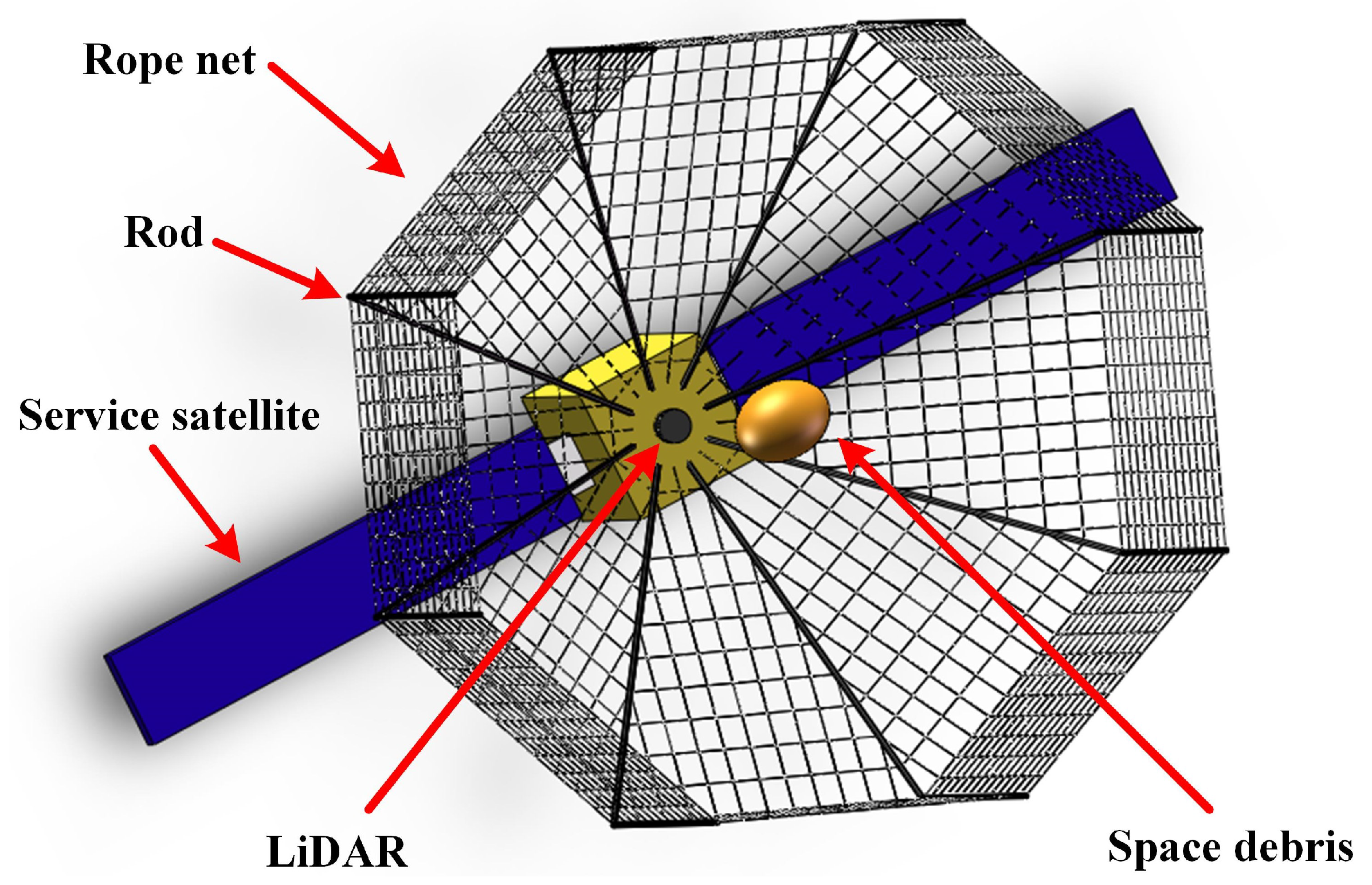
According to the preceding analysis, the “non-contact” method can only identify the normalized parameters of debris, which cannot provide sufficient information for detumbling and capture operations. However, the “contact” method is frequently based on mechanisms such as mechanical arms or elastic rods, or space tethers that have strong connections with satellites, which are frequently prone to potential safety hazards. Therefore, in order to solve the above problems, this paper proposes an identification method for large space debris dynamic parameters based on rope net flexible collision and vision, which is shown in Figure 1.
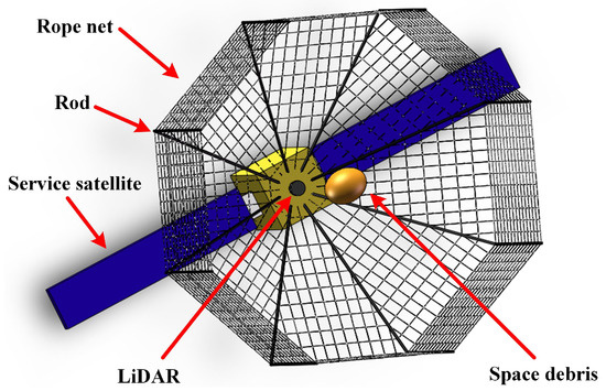
Figure 1.
The schematic diagram of the estimation method of full dynamic parameters of large space debris based on rope net flexible collision and vision.
In this method, the identification process for the debris’s parameters is regarded as an unconstrained optimization problem of redundant motion and dynamic equations, and the L-M algorithm is used to optimize the dynamic parameters. The process of the identification method is divided into two steps:
- (a)
- The normalization parameter identification before collision;
- (b)
- The true value calculation of the dynamic parameter after collision.
Before the collision, the point cloud of debris is collected by LiDAR, and the motion parameters of the debris and transformation matrix of point clouds are calculated through point cloud registration. The real-time position of the center of mass is estimated based on the motion equation and the feature points’ position. In addition, the transformation relationship from the LiDAR coordinate system to the debris-fixed coordinate system is derived through the initial position of mass center and transformation matrix of the point cloud. Using the transformation relationship, the debris movement data is then transferred to the debris-fixed coordinate system, and the normalized inertia tensor, normalized kinetic energy and direction of angular momentum are estimated based on the dynamics model and dynamic parameter characteristics of the debris. After the collision, the debris, satellite and rope net are regarded as a unified system, and the real-time momentum characteristics of the rope net which are difficult to measure are calculated based on the position change of the point cloud of the rope net node. And the true values of the mass and the principal inertia moment of the debris are estimated through the conservation of the linear momentum and angular momentum of the whole system. Then, the true values of the inertia moment are substituted into the normalized parameters to obtain the true values of the kinetic energy and momentum of the debris, and all dynamic parameters of large space debris are estimated accurately and in real time. The simulations of estimating dynamic parameters were carried out, and the results prove the real-time accuracy and high precision of our method.
2. Coordinate System and Space Debris Movement Description
The notations used in our paper will be defined in this section. In this paper, the vector and matrix are written in lowercase bold and uppercase bold respectively. The coordinate system is written in uppercase font. If the coordinate system symbol appears in the lower right corner label of a vector or matrix label, it indicates that it is a projection of the vector or matrix under the coordinate, for example, indicates the projection of the vector in the coordinate system C. In this paper, the identification process of dynamic parameters of space debris is regarded as the detection task of target debris T by service satellite S. The central principal axis frame of the target space debris T is located at the debris centroid , and its z axis points to the direction of minimum moment of inertia of the large space debris, x axis points to the direction of maximum moment of inertia, and the y axis direction is determined by the right-hand rule. The coordinate system T is related to the mass distribution of the rigid body, so it is a conjoined coordinate system of space debris. The origin of the rope net coordinate system N is established at the middle node on the left side of the net, with its y axis pointing to the upper side of the rope net, x axis pointing to the right side of the rope net, and the z axis direction determined by the right-handed rule. The origin of the LiDAR coordinate system C is established in the center of the LiDAR, with its z axis parallel to the normal direction of the solar wing of the satellite, y axis pointing to the upper part of the LiDAR, and x axis direction also determined by the right-hand rule. At the same time, the debris fixed coordinate system B is established at the initial sampling time of the LiDAR, and its origin is located at the center of mass of debris, and the directions of each axis are the same as those of the LiDAR coordinate system. If the rotation matrix of debris at each timepoint is known, it is easy to obtain the orientation of the axis of B in C at each timepoint. In fact, the rotation matrix can be easily calculated by using the point cloud registration (such as ICP, D2D-NDT algorithm), which will be discussed in Section 3. Set the inertial coordinate system , the origin of which is located in the center of the Earth, the axis points to the vernal equinox in the equatorial plane, the axis is 90° to the east in the equatorial plane, and the axis coincides with the Earth’s rotation axis. The origin of the satellite coordinate system S coincides with the center of mass of the inertial sensor carried by the satellite, and the axis pointing is determined by the sensor setting and the coordinate system S is known. The coordinate system is shown in Figure 2.
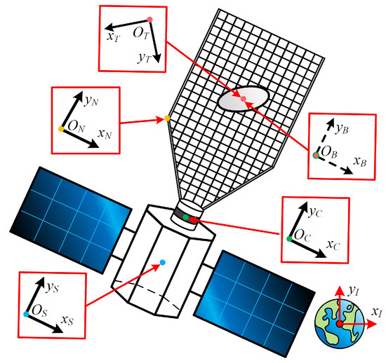
Figure 2.
Coordinate system.
The rotation transformation of a rigid body between coordinate systems can be expressed in the form of the following rotation matrix:
where is a 3 × 3 rotation matrix, and G and H represent any coordinate system, which represents the transformation matrix from frame G to frame H. In this paper, the angle–axis method is used to describe the rotation. According to Euler’s rotation theorem, the rotation of a rigid body can be regarded as an infinitely small angle around the instantaneous axis , that is, the angle-axis method representation can be obtained. In this paper, the motion data of space debris are collected by LiDAR, the sampling frequency is 10 FPS, and the rotation speed of space debris is less than 3 rad/s, which accords with the assumption of a small rotation angle. Therefore, the rotation is described by the angle–axis method in this paper. Because of the constraint that the modulus of is equal to 1, four unknowns can be reduced to three. The conversion formula between the angle–axis method and the rotation matrix is:
The projection of translation transformation vector in coordinate system C is:
The transformation between coordinate systems is described by transformation matrix , which can be expressed by direction cosine matrix and translation transformation vector :
It can be seen from the coordinate system setting that the transformation matrix and between the satellite frame S and LiDAR frame C is known. As the deformation of the rod is small during the collision between the debris and the rope net, it is considered as a rigid rod, and the transformation matrix of the LiDAR coordinate system and the coordinate system of the rope net is also known. According to the measurement data of the star LiDAR carried by the satellite, the transformation matrix between the inertial coordinate system I and the satellite coordinate system S is also known.
The Euler–Poinsot model is used for space debris dynamics modeling. In this model, the non-cooperative object is considered as a rigid body rotating around the center of mass without torque, and the model is:
where is the inertia tensor matrix of debris, which is related to the mass distribution of debris. As a result, its projection in a certain debris-fixed coordinate system is constant. is the angular velocity of debris and is the angular acceleration of debris. After projecting to the principal axis coordinate system T, it will be changed from six parameters to three parameters, from which the moment of momentum integral and angular kinetic energy integral with simple forms can be obtained. Since it is assumed that the space debris is not affected by external torque, its motion is constrained by conservation of angular kinetic energy and conservation of momentum moment; its integral can be expressed as an elliptic equation:
where A, B and C are the central moments of inertia, and E and L are the constant angular kinetic energy and angular momentum of the debris. According to the constraints, it can be known that the end of the angular velocity vector should always move at the intersection of two ellipsoids (angular kinetic energy ellipsoid and momentum moment ellipsoid) [7]. Considering the space debris as the general case of three-axis principal moment of inertia asymmetry and low energy (that is, the relative value of kinetic energy is less than the relative value of momentum ), and the simulation of the low energy state was carried out. The debris geometry and inertia parameters used in its simulation are shown in Table 1. During the simulation process, a 2.949 × 10 Nm torque of 0.1 s was applied to the space debris to generates a spin motion of [0.105, 1.053, 0.211] rad/s for space debris. And a perturbation torque with 4 × 10 Nm in the y-axis direction was applied to the satellite from 3.8 s to 3.81 s to simulate the impact of a small object on the debris, and showed a low-energy state characteristic after 4 s of stabilization. The Polhode analysis of the debris at this timepoint is shown in Figure 3.

Table 1.
Parameters of the debris.
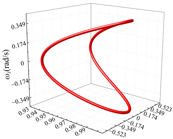
Figure 3.
The Polhode analysis of the space debris.
Based on the coordinate systems and debris dynamic model described above, the next chapter will carry out the identification method for full space debris dynamic parameters.
3. Identification Method for Full Dynamic Parameters
In this section, the identification method based on rope net flexible collision and vision will be discussed. It is divided into two steps: first, before the collision, the LiDAR is used to scan point clouds of the debris, and then the rotation and translation motion data of the debris are calculated. Furthermore, based on motion data and the debris dynamics model, optimization calculations are performed to obtain the center of mass of the debris with the normalized inertia tensor, normalized angular momentum. It should be noted that the literature [11] shows that there is always an unmeasurable parameter when identifying the 6-DOF using the non-contact method, with the result that only normalized inertia tensor and normalized angular momentum can be solved without contact with space debris. After the normalized parameter identification, collisions of unilateral capture nets with debris are carried out and parameter true value identification is performed. Due to the time-varying contact area of rope net, collision force and debris movement state during collision, there is an excessive number of parameters to identify, which makes it difficult to identify them efficiently. And it is difficult to collect point clouds by LiDAR because of the occlusion of the area. Therefore, the collision process is not considered in the paper, only the motion state of debris, satellite and rope net prior to and after the collision is considered. As the process of identification–collision–identification takes little time, the influence of the low perturbing force in space can be ignored; the debris–satellite–rope net system maintains the conservation of angular momentum. Therefore, the changes in subsystem angular momentum parameters before and after collision can be used to identify the true values of dynamic parameters efficiently, and to finally solve all the dynamic parameters needed for the debris detumbling and capture process. The two-step identification method of full debris dynamic parameters is described below.
3.1. Identification of the Center of Mass and Normalized Dynamic Parameters Based on Vision
In order to reduce the influence of extreme optical environment in space, the point cloud data of the large space debris is obtained by LiDAR. The D2D-NDT algorithm is used to solve the point cloud registration to improve the calculation efficiency of debris pose [19]. Let the source point cloud at time i be , and the target point cloud at time be , then the calculation for the point cloud registration is as follows:
where are the transformation parameters to be optimized, is the transformed mean vector distance, is the mean of each Gaussian component, is rotation matrix and is translation vector. is the covariance of each Gaussian component, where . And and are the number of Gaussian components in the NDT model at time i and time respectively; and are regularization factors. After the point cloud registration, the angular velocity , linear velocity , angular acceleration and linear acceleration of the debris can be obtained from the central difference of the transformation matrix at time , i and :
where the value of can be the rotation vector or the translation vector , and is the time interval. The angle can be obtained from Equation (2) and the normalization condition of the vector . Expanding the right-hand side of Equation (2) yields:
The normalization condition of the unit vector can be expressed as follows:
Then, from Equations (11) and (12), the expression for angle can be derived:
where denotes the trace of the matrix . The motion of the debris can be divided into rotation motion around the center of mass and translation motion of the center of mass, and the motion of characteristic point can be described as:
where is the linear velocity of the feature point m, which can be obtained by the position difference of the feature point at two moments. is the distance from the feature point to the center of mass. is the translation speed of the center of mass (based on the motion characteristics of debris). Then, the distance from the feature point to the mass center at time i can be obtained from (14). Then, using the locations of multiple feature points measured at moment i as the center of the sphere and the distance as the radius, the spheres can be created. It is known that the center of mass of the debris should be located at the intersection of spheres under the condition of accurate measurement. However, due to the measurement error of LiDAR, the spherical surface essentially cannot intersect at one point. Therefore, the center of mass should be located at the point with the shortest distance from every spherical surface in space and then it can be transformed into an unconstrained optimization problem, and then the objective function can be established:
where is location of the center of mass. Then, the more accurate centroid position at time i can be obtained by using the positions of multiple feature point pairs. Then, a debris-fixed coordinate system B can be established based on the centroid position calculated at the initial sampling time and its origin is located at the mass center of debris, and the directions of each axis are the same as those of C. According to the definition, the initial rotation matrix from the coordinate B to the coordinate C is the identity matrix, and the motion parameters can be projected into the B coordinate system through this matrix in the initial timepoint. At the same time, the angular velocity and angular acceleration vectors at each timepoint can be easily transformed into the debris-fixed coordinate system B through the rotation matrix and the position of mass center which is calculated at each timepoint:
where or . Then, the projection of angular velocity and angular acceleration of space debris in the debris-fixed coordinate system B can be obtained. Using the angular velocity and angular acceleration at multiple times, the inertia tensor matrix is optimized based on the torque-free Euler–Poinsot model:
The basic form of inertia tensor contains six independent parameters, including the three moments of inertia relative to three axes and the three products of inertia, which represents the mass distribution of debris in the coordinate system. However, due to the incomplete observation of the non-contact method, it can only measure the normalized five parameters. When each axis in the coordinate system points to the principal axis of inertia, that is, in the T coordinate system, the normalized inertia tensor matrix becomes a diagonal matrix containing only two normalized principal moments of inertia, which can be estimated by the dyadic coordinate transformation:
where (); at the same time, the transformation matrix between coordinate system T and the coordinate system M can be estimated from the above transformation (because the coordinate system B and the coordinate system T are debris-fixed coordinate systems, the matrix is constant). Because is known in the process of estimating the center of mass, can finally be known. Then, the angular velocity and the angular acceleration vector in the principal axis coordinate system T at each moment can be finally known. Therefore, the normalized parameters can be estimated through the conservation of the normalized kinetic energy and the normalized momentum:
where is the normalized angular kinetic energy and is the normalized angular momentum, which is known to be constant by definition. Then, the values of these two normalized parameters can be optimized by using the angular velocity data at multiple timepoints. After the estimation of the value of the principal moment of inertia by the collision, the angular kinetic energy and angular momentum true values can be obtained by using the calculation results of Formulas (20) and (21). However, the momentum is a vector, and the modulus only cannot be applied to the detumbling operation. It is necessary to obtain the identification method for the angular momentum direction. According to Poinsot’s geometric explanation of Euler–Poinsot motion, the angular velocity projection in LiDAR coordinate system I should be on the same plane and the direction of the angular momentum is in the vertical direction from the center of mass to the plane. Therefore, the normalized angular momentum of space debris can be obtained by solving the normal vector of the plane:
where are unit vectors indicating the direction of the angular momentum vector. And from the star cameras and satellite orbit data, the rotation matrix from the satellite coordinate C to the inertial coordinate I can be obtained more easily, i.e., the angular velocity data under C can be used to solve Equation (22). From the above optimization function to , the real-time position of the center of mass, normalized inertia tensor, normalized kinetic energy, normalized angular momentum and the direction of angular momentum of the debris can be estimated based on the L-M algorithm. In the following, the true value of the space debris dynamic parameters will be identified based on the comparison of the parameters before and after the collision.
3.2. Estimation of the True Value of Full Dynamic Parameters Based on Rope Net Flexible Collision and Vision
Spacecraft, rope net and space debris are regarded as the whole system in this paper, which is not disturbed by external forces before, during or after collision (short identification time, ignoring the effect of spatial perturbation). And the system maintains the conservation of angular momentum and linear momentum. Furthermore, the following two equations can be established from the conservation of momentum before and after the collision:
where is the linear momentum, is the angular momentum, the lower corner marks , and denote the relevant parameters of spacecraft, debris and capture net, respectively, and the superscripts (0) and (1) denote the parameters before collision and after collision, respectively. If the above formula is projected into the coordinate system C, the linear momentum and angular momentum of the debris before and after the collision can be measured by the LiDAR, and the satellite-related motion parameters can be obtained by the inertial sensor carried by the satellite; only , , and in the above formula are unknown, and only one parameter of the inertia tensor is unknown after the solving of the previous Formula (18). In order to estimate the inertial parameters of the debris by Equations (23) and (24), it is necessary to estimate the momentum parameters and .
Because the flexible deformation process of the rope net is complicated, it is difficult to obtain the analytical solution. Therefore, most of the existing dynamic calculation methods use beam elements, solid elements and other models to discretize its structure in space, and use finite-element method for iterative calculation to obtain more accurate dynamic characteristics of the rope net. However, the combination of discrete finite element method and existing identification method of dynamic parameter is difficult, and it takes a long time, especially for the rope net of several meters in this paper. The number of elements can reach tens of thousands and the calculation time is extremely long; it cannot be applied to the process of detumbling and capture of space debris with high identification efficiency demand. Therefore, this paper simplifies its calculation in order to improve the efficiency of identification. Because the collision process is instantaneous, the friction force on the rope net is limited and the rope net material has a certain stiffness; its angular momentum is limited. Thus, the angular momentum of the rope net is ignored in the calculation of Equation (24) (but the influence of angular momentum brought by the overall movement of the satellite needs to be considered). However, the rod can ignore its own deformation because of its high rigidity. Therefore, the whole movement of the net can be discretized to the nodes of the rope. The location of the node can be obtained by LiDAR, the velocity characteristics of the node are calculated by Equation (9), and the mass of the rope network is uniformly discretized to the node. The linear momentum of the whole rope net can be estimated by the nodes’ mass and position, and the true values of the dynamic parameters can finally be obtained through Equations (23) and (24).
As can be observed from the analysis above, the key challenge of the current calculation is to estimate the nodes’ location using the collected rope points cloud. In this paper, a fast search method for the node position is proposed, which is divided into five steps:
- (1)
- Point cloud projection: Since it is assumed that the rod of the rope net is rigid and does not deform, the transformation relationship between the LiDAR coordinate system C and the rope net two-dimensional coordinate system N is known, and the projection coordinates of the node point cloud in N can be obtained:
- (2)
- Area division: The fixed point of the rope net on the rod is the starting and ending point of the segmentation, the node of the rope net before deformation is the center, the mesh side length is the division side length, and the area division is performed.
- (3)
- Boundary point determination: In order to improve the speed of identifying the position of the nodes, this paper does not use the commonly used edge extraction algorithm and adopts a cyclic identification method of boundary point determination–intersection point identification of boundary points–regional redividing. For the determination of boundary points, in order to improve the search efficiency, a boundary point search method with “” strategy is used, because the random error of ranging is known when the LiDAR is calibrated on the ground and then the point closest to the boundary can be found in the area inside the boundary. Then, the point cloud can be approximately regarded as being located on the same straight line through the region and a straight line can be fitted:The approximate boundary intersection point is found by solving the intersection point between the fitted straight line and the boundary.
- (4)
- Identification of “node”: Use straight lines to connect the left and right boundary intersection points, and the upper and lower boundary intersection points, and find out the intersection point of the two lines. The coordinates of the intersection points are the once estimated coordinates of the nodes.
- (5)
- Area redividing: taking the obtained estimated node as the center, taking 1/8 of the existing grid length as the side length, redivide the area. Repeat steps 2, 3 and 4, and finally get more accurate coordinates of the rope net node. Because the length of a single rope net mesh is about 0.5 m, the diameter of the rope net is 0.02 m, the rope net is relatively rigid, and there is the stretching effect of the rod; thus, the rope net will not be deformed greatly after the collision. Therefore, it only needs to be repeated three times to accurately identify the node position of the rope net and the relevant proof will be given in the subsequent simulation. The identification process of rope net node is shown as Figure 4.
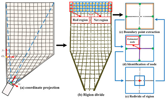 Figure 4. The identification process of rope net node.
Then, a more accurate position of the rope net node can be obtained through the above steps. By replacing the position data of rope network nodes at multiple moments into Equations (22) and (23) for optimization calculation, the debris mass and the inertia tensor unknown C can be obtained:
where is the transformation matrix between the inertial coordinate system I and the LiDAR coordinate system C, which can be obtained by multiplying and , and can be obtained according to the measurement data of the star camera carried by the satellite. Then, the calculated debris mass is substituted into (23) to obtain the true value of the linear moment of the debris, and the obtained principal moment of inertia C is substituted into Equations (20) and (21) to obtain the module of the angular kinetic energy and the angular momentum, which are combined with Equation (22) to finally obtain the true value of the angular momentum vector of the system. Through Equations (1)–(32), the true quantities of the full dynamic parameters of debris can be obtained, and the accurate data reference can be provided for subsequent detumbling and capture operations.
4. Simulation of Full Dynamic Parameters’ Identification
4.1. Simulation Parameter Setting
In order to verify the effectiveness of our method, the simulation of the dynamic parameters’ identification was carried out. Referring to “the History of On-Orbit Satellite Fragmentation 15th Edition” published by NASA [20], the large space debris’s size is set to be an asymmetric ellipsoid of 0.65 m × 0.7 m × 0.9 m and a mass of 1715.2 kg. The principal moments of inertia of the debris are 445.98 kg·m, 442.80 kg·m and 313.04 kg·m, respectively, and the normalized principal moments of inertia are 1.425, 1.351 and 1, respectively. The diameter of the net is 0.004 m, density is 1430 kg·m, the Poisson ratio is 0.3 and the modulus of elasticity is 12 Gpa. The mass of the satellite is 3178.15, and the principal moments of inertia of the debris are 690.13 kg·m, 671.36 kg·m and 543.71 kg·m. The initial angular velocity is rad/s and the initial relative linear velocity is m/s in order to simulate the satellite remaining at approximate relative rest in relation to the debris before the collision. And the linear velocity of the satellite is set to m/s during the collision to simulate the process of collision. The parameters of the debris are shown in Table 1. The LiDAR are set with reference to C-Fans-256 LiDAR, the ranging random error (1) is 2 cm(@20 m), the sampling frequency is 10 Hz and the FOV is 150° × 30° (in this paper, it is assumed that the rotating head is used to change the attitude of the sensor to achieve the coverage of all sides of the rope net, which can be realized more easily; because the problem is simplified to the collision problem of the single side rope net, so the design of the head is not elaborated), and the resolution is 0.09° × 0.12°. A total of 100 simulations were performed and the results shown below are the closest to the mean. The simulation parameters are shown in Table 1, Table 2 and Table 3.
Table 2.
Parameters of the rope net and the the service satellite.
Table 3.
Parameters of the sensors.
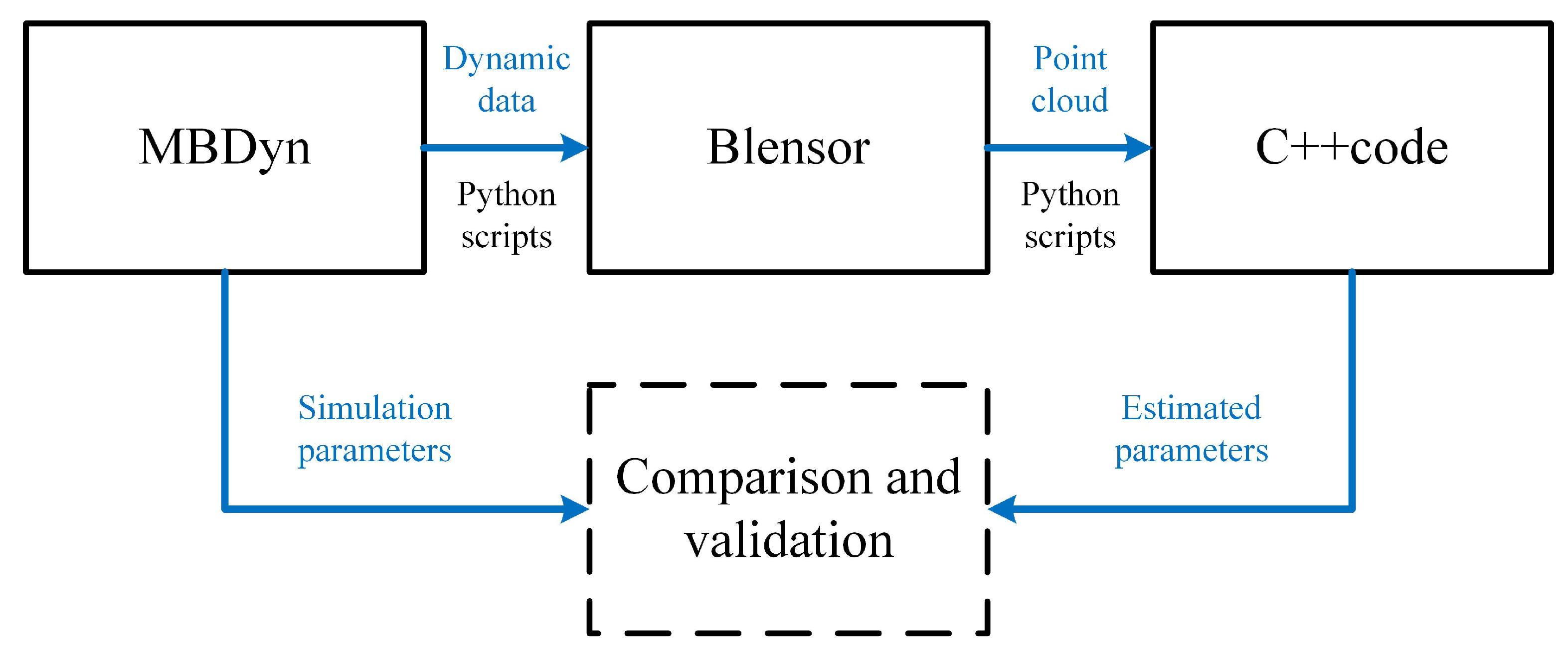
The MBDyn sofware, developed by our research group, is adopted to calculate the dynamic of the debris and rope net dynamics. It has rich flexible body calculation codes (such as ANCF and other FEM models suitable for rope nets), which can meet the requirements in this paper. After the dynamic calculation, MBDyn can reconstruct the whole satellite 3D model at each moment by using the coordinates of the node and the deformation parameters of the element. Then, the reconstructed model is imported into Blensor through Python script code, photographed by LiDAR, and the point cloud data is output to the algorithm C++ code of this paper for dynamic parameter identification. Comparing the results of our method with the calculation results of MBDyn, the effectiveness of the proposed method is verified. The simulation flow is shown in Figure 5.
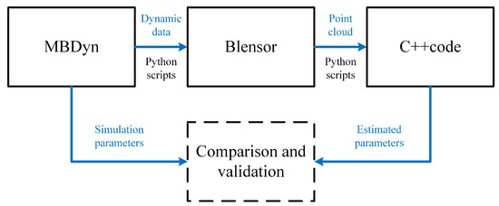
Figure 5.
Simulation flow.
4.2. Hypothesis Analysis
In response to the assumption of space debris and rope net momentum adopted in this article, this section provides a reasonable proof of this assumption to demonstrate the effectiveness of the proposed method.
4.2.1. Analysis of the Torque-Free Assumption of the Space Debris
For the dynamic modeling of space debris, this paper ignores the influence of the spatial perturbation force on space debris in a short period and adopts the Euler–Poinsot model for debris dynamic modeling, which is the modeling method used in most of the paper. The correctness of the assumption will be explored through numerical simulations in this section. The dimensions and inertial parameters of the space debris used in the simulation are referenced in Table 1. Meanwhile, from the data in the [20], it can be seen that the space debris has the highest orbital density near 825 km. Thus this section of the simulation puts the debris at that orbital altitude. At the same time, the debris orbit parameters are set with reference to the payload debris of NOAA-8. Referring to [21], J perturbation, perturbation of sun and the moon, Earth tide and ocean tide, atmospheric drag, and solar radiation pressure were set. The total simulation time is 500 s, and the simulation results of the debris’s angular kinetic energy and angular momentum are shown in Figure 6.
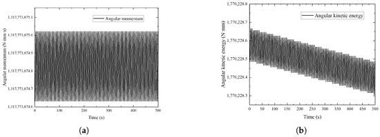
Figure 6.
Simulation analysis of the torque-free assumption. (a) Changes in angular kinetic energy of the debris after 500 s. (b) Changes in angular momentum of the debris after 500 s.
It can be seen that, after 500 s, the angular kinetic energy of the system only decreased by 1.9810%, angular momentum only decreased by 1.5210%, and the periodic oscillation amplitude of the system kinetic energy within 500 s only accounts for 8.4710% of the total angular kinetic energy, with a momentum periodic oscillation amplitude accounting for 2.6610% of the total angular momentum. Therefore, the influence of spatial perturbation torque on the dynamic characteristics of debris in a short period of time is extremely weak, proving the correctness of this hypothesis.
4.2.2. Analysis of the Torque-Free Assumption of the Rope Net
In this paper, the dynamics calculation process of the rope network adopts the MBdyn software developed by our group, which has been successfully applied in the fields of nonlinear dynamics analysis and control of large flexible structures, rope driven snake manipulator and space dobby robots, etc. [22,23,24,25]. In this paper, the ANCF method code in the MBdyn software is adopted for rope net calculation, in which unit generalized coordinates contain the node position and gradient at the node, i.e.:
where is the shape function. The unit dynamic equations were derived using D’Alembert’s principle:
where is the elastic force, while is the external force action. And the dynamics model of the rope net system is constructed:
where is the mass matrix, is the generalized coordinate, the generalized force vector, is the constraint equation, and is the strain energy. Since the rope net dynamics model in this paper is only used in the numerical simulation and the identification method for the dynamic parameter mentioned in the paper is weakly related, it will not be repeated. The detailed modeling process can be referred to in the authors’ published paper [22].
Since the ANCF method describes the deformation, kinetic energy and internal energy of each unit, it is difficult to achieve a more efficient calculation when the method is applied to models with more units. For example, in this paper, the size of the rope net is 5.78 m × 12 m and at least 13,800 meshes are required to ensure that the calculation process is not divergence. In our previous work, the ANCF method was applied to the parameter identification, which achieved good computational accuracy, but the single identification time of the dynamic characteristics of the rope net was more than 30 s, which made it difficult to realize higher computational efficiency. In order to improve the computational efficiency of dynamic parameter identification, the following assumptions are used in this paper:
- (a)
- The angular momentum of the rope net node is ignored; only the linear momentum of the rope net is considered. (But the influence of angular momentum brought by the overall movement of the system needs to be considered.)
- (b)
- The mass of the rope network is uniformly discretized to the node. The linear momentum of the rope net subsystem is equal to the sum of the linear momentum of the motion with the satellite and the linear momentum of the deformation.
For the above assumption (a), due to the target debris and rope net collision process being short (less than 0.5 s), the friction between the rope net and debris is smaller compared to the contact collision force, so the friction force on the rope net movement has less impact. Due to the smaller mesh size of the single rope net (0.48 m0.5 m) and the fixed boundary node on the rigid rod, the rope net meshes have some stiffness. Hence, the torsional movement of the rope net node is limited after the collision and thus its angular momentum is limited. Therefore, the angular momentum of the rope mesh nodes is ignored (but not the rotation of the rope mesh subsystem with the satellite) to improve the computational efficiency of the identification process. At the same time, in order to quickly calculate the overall linear momentum of the net, the reconstruction of each unit was not carried out but distributed the mass of the rope mesh to the nodes of the rope mesh equally, and collected the coordinate positions of the nodes of the rope mesh to improve the efficiency of the calculation of linear momentum, i.e., assumption (b). The main reason for making assumption (b) is to consider that the individual rope mesh has a certain stiffness, so the deformation of the rope mesh is linear and the maximum deformation is concentrated at the nodes. Therefore, we made assumption (b).
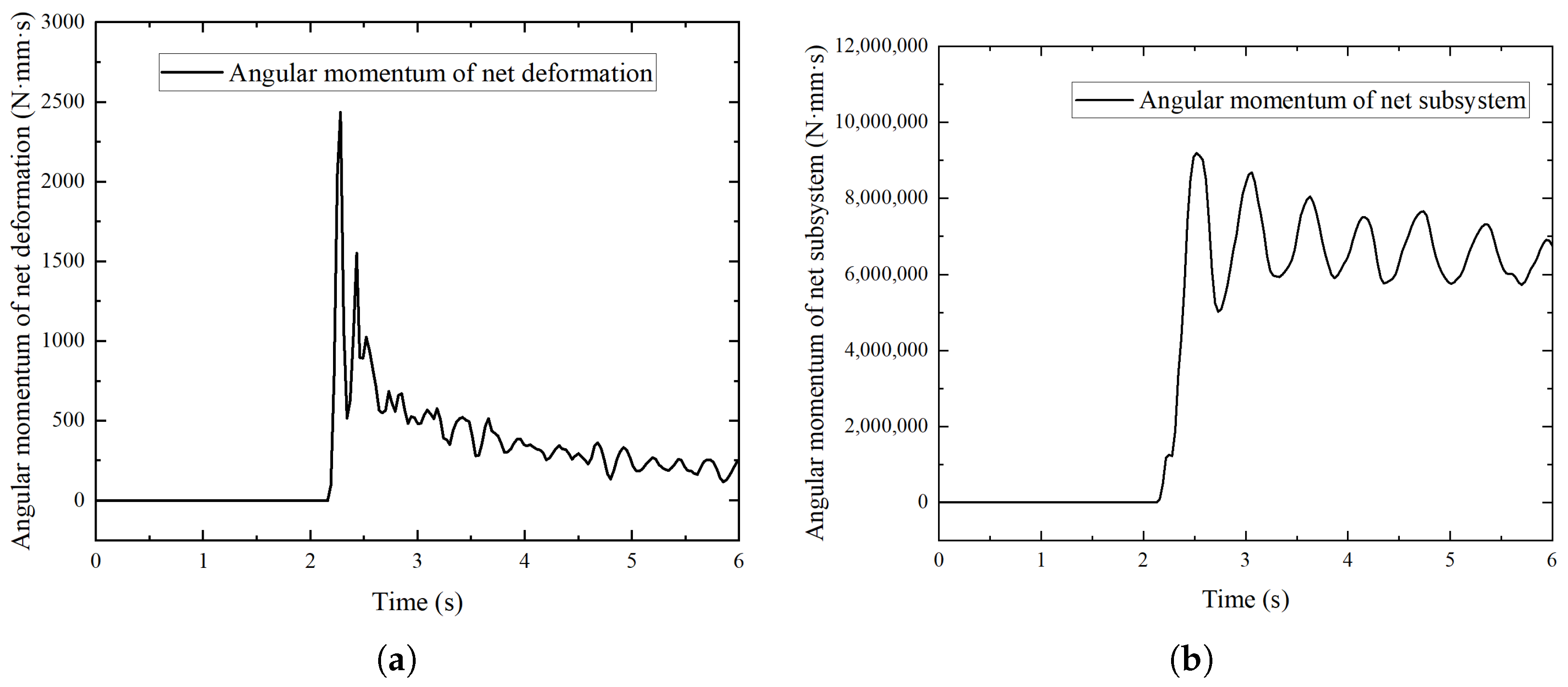
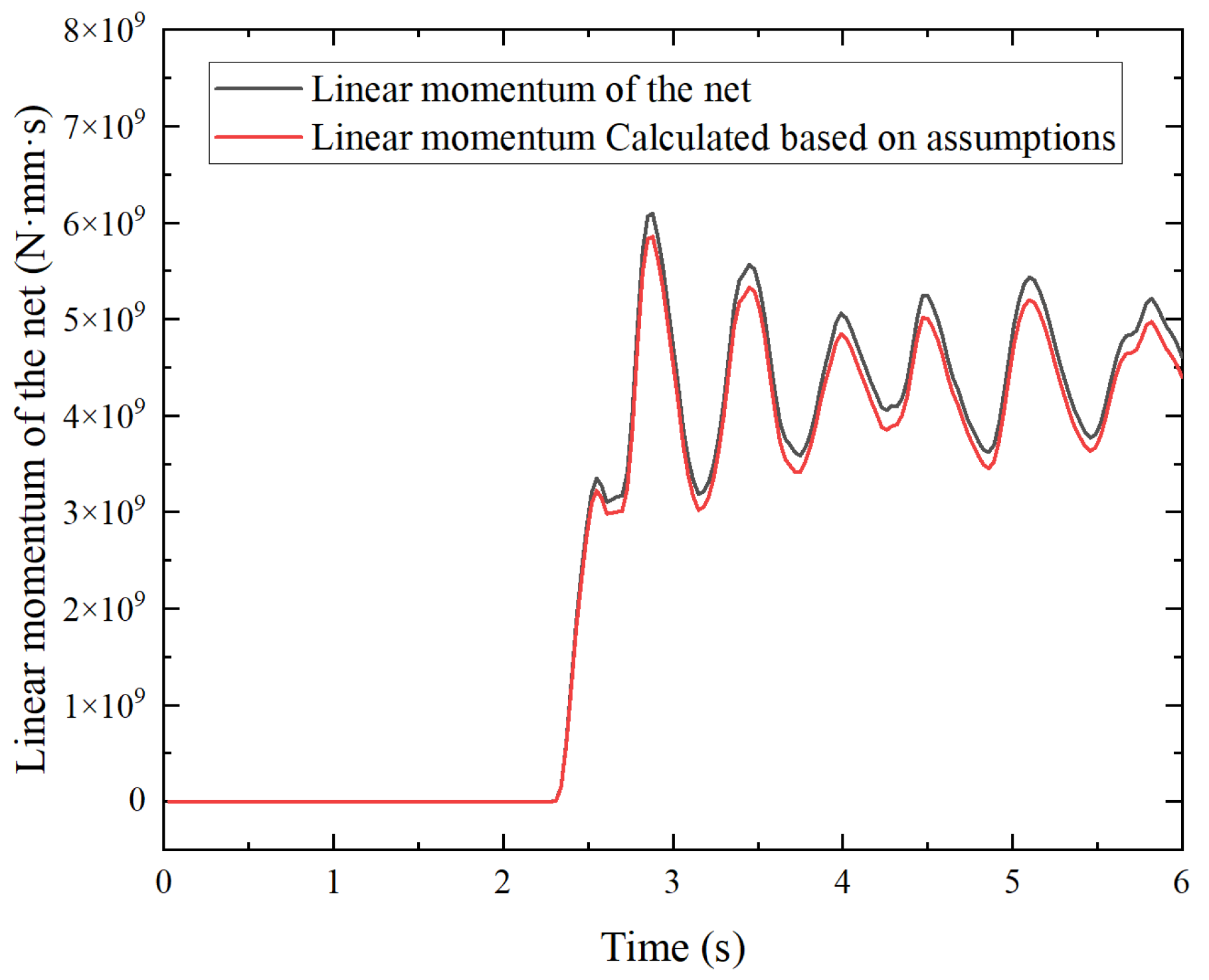
For the rope mesh hypothesis, a simulation study of the collision between debris and rope mesh was carried out. The parameters of the debris and flexible rope net are shown in Table 1 and Table 2, and the angular momentum and linear momentum of the rope net after collision are shown in Figure 7. It can be seen that, after the collision, most of the angular momentum of the rope net is generated by the cooperative motion with the satellite, while the angular momentum generated by the deformation of the rope during the LiDAR acquisition process only accounts for 0.39% to 0.65% of the subsystem’s angular momentum and therefore it can be ignored in the calculation process. And the simulation of the linear momentum of the rope net nodes is shown in Figure 8. It can be seen that the maximum error of the calculated momentum by this assumption is 3.79%, which proves the simplification made to the rope net in this paper has little effect on the calculation process.
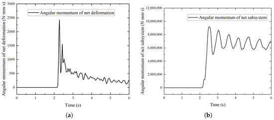
Figure 7.
Simulation analysis of angular momentum of the rope net. (a) Angular momentum due to deformation of rope mesh nodes. (b) Overall angular momentum of the rope net.
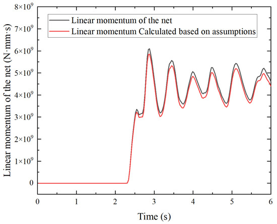
Figure 8.
Results of simulation of the assumption of net linear momentum.
At the same time, the amount of data collected during the identification process on the impact of the error was calculated; the results are shown in Table 4. It can be seen that, when the collection time is greater than 300 s, the computational accuracy of the identification algorithm no longer grows, while when it is less than 300 s it is difficult for the calculation error to meet the method’s demand. Hence, the amount of data collected has a greater impact on system identification. Therefore, in this paper, the relevant parameters are solved after 300 s of data collection.
Table 4.
Impact of the amount of data collected on identification.
4.3. Identification of Centroid and Normalized Dynamic Parameters
Firstly, the solving effect of the DTD-NDT algorithm is evaluated, the point cloud sampling results for the two moments are shown in Table 5. The average error of the solution in the simulation is 8.49% and the average calculation time is 0.11 s. Although this algorithm is faster than other point cloud registration algorithms, it is still not able to achieve real-time measurements as with contact sensors. Since parameter identification is considered as an unconstrained optimization problem in this paper, the calculation accuracy of the method can be guaranteed only when the number of samples is sufficient. But it is difficult for the LiDAR to collect enough sample data in a short period of time. Therefore, considering the influence of factors such as point cloud registration time and the registration errors, 300 s data are collected before the normalized parameters are calculated to ensure the accuracy of the subsequent identification algorithm.
Table 5.
Simulation error of the DTD-NDT algorithm.
The center of mass position is identified for the initial moment and the identification results are shown in Equation (7). It can be seen that the average error of the mass center identification is less than 0.81% after 0.16 s, and the results of mass center identification for the whole process of debris motion before and after collision are shown in Figure 9, Figure 10 and Table 6. It can be seen that the average error of a single centroid is less than 0.5%, the maximum error is less than 1.3% and the calculation time is below 0.17 s. The simulation results show that the identification method can identify the real-time and accurate position of the center of mass.
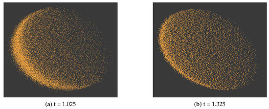
Figure 9.
Simulation results: the point cloud sampling.
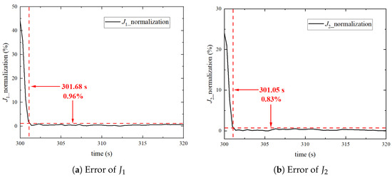
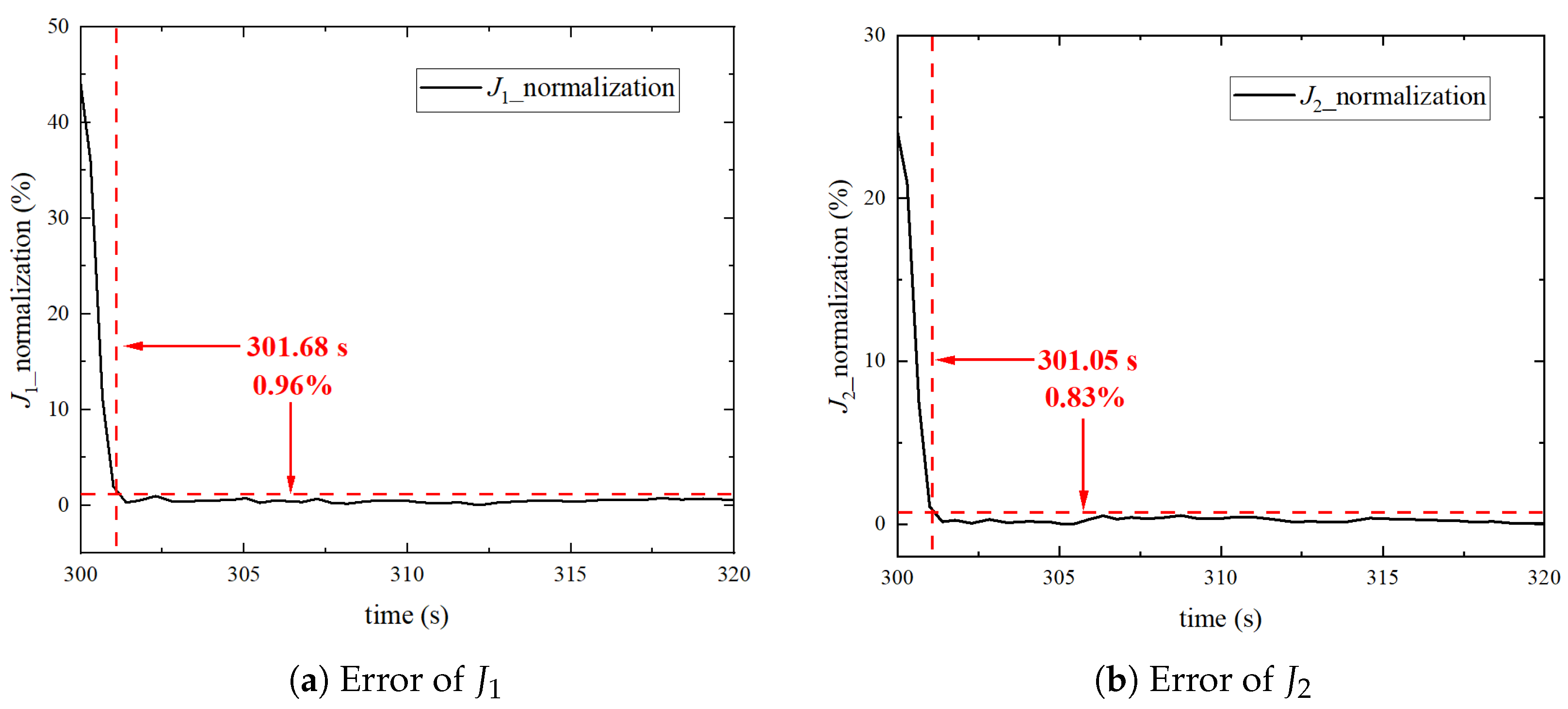
Figure 10.
Simulation results: error of normalized principal moment of inertia.
Table 6.
Identification results of the center of mass.
The identification results of the inertia ratios are shown in Figure 10. It can be seen that the error of converges to less than 0.96% after 301.68 s (actual identification time 1.68 s) and the error of converges to less than 0.83% after 301.05 s (actual identification time 1.05 s). It is proved that the method proposed in this paper can quickly identify the accurate inertia ratios under the condition of sufficient data.
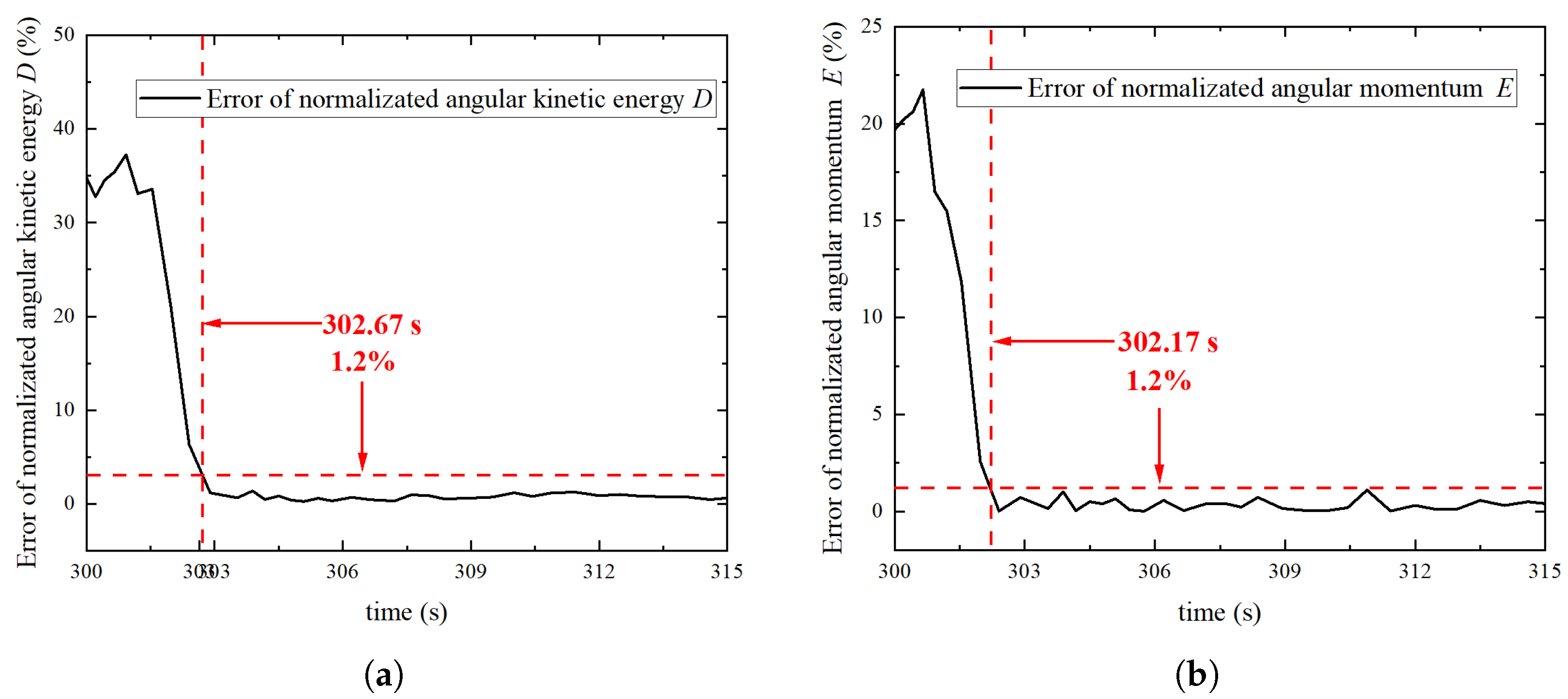
After the normalized inertia tensor is obtained, the normalized angular kinetic energy D and the normalized angular momentum F can be solved. The results are shown in Figure 11 and Figure 12, and Table 7. It can be seen that the error of normalized angular kinetic energy D converges below 1.2% when the simulation reaches 302.67 s (the actual identification time is 2.67 s). At 302.17 s (actual identification time is 2.17 s), the error of normalized angular momentum F converges to less than 1.2%. And, as shown in Figure 13b, when the actual identification time reaches 3.77 s, the triaxial errors of the angular momentum direction are all below 0.61%, which proves that the proposed method can identify the normalized parameters of space debris accurately and efficiently. Compared with the identification of the normalized principal moment of inertia, the calculation speed of parameters D and F is faster, mainly because each equation contains only one unknown, so the calculation speed of its equations is faster than that of J.
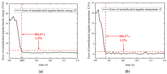
Figure 11.
Simulation results: identification of the normalized parameters. (a) Error of the normalized angular kinetic energy. (b) Error of the normalized angular momentum.
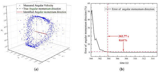
Figure 12.
Simulation results: identification of the direction of the angular momentum. (a) Identification results of the direction of the angular momentum. (b) Error of the direction of the angular momentum.
Table 7.
Simulation results: statistical results of the normalized angular momentum calculation errors.
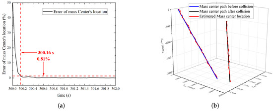
Figure 13.
Simulation results: error of mass center. (a) Error of initial mass center. (b) Error of the trajectory of the mass center.
4.4. Simulation of the Estimation of Dynamic Parameters’ True Values
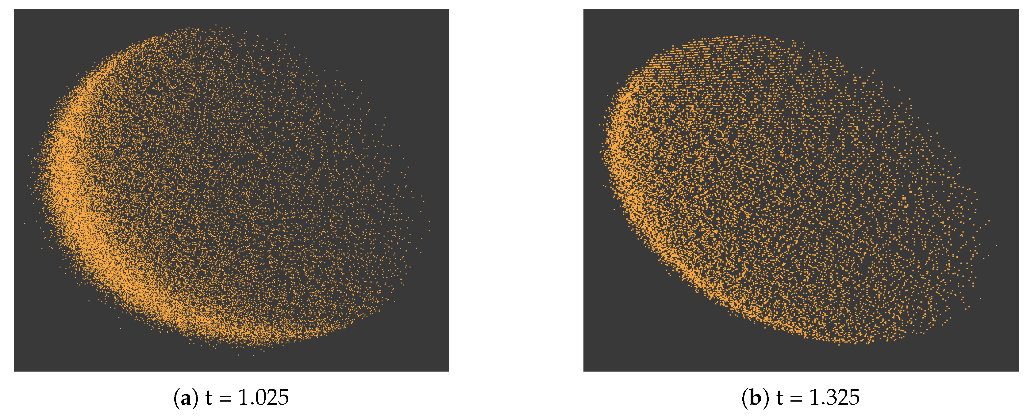
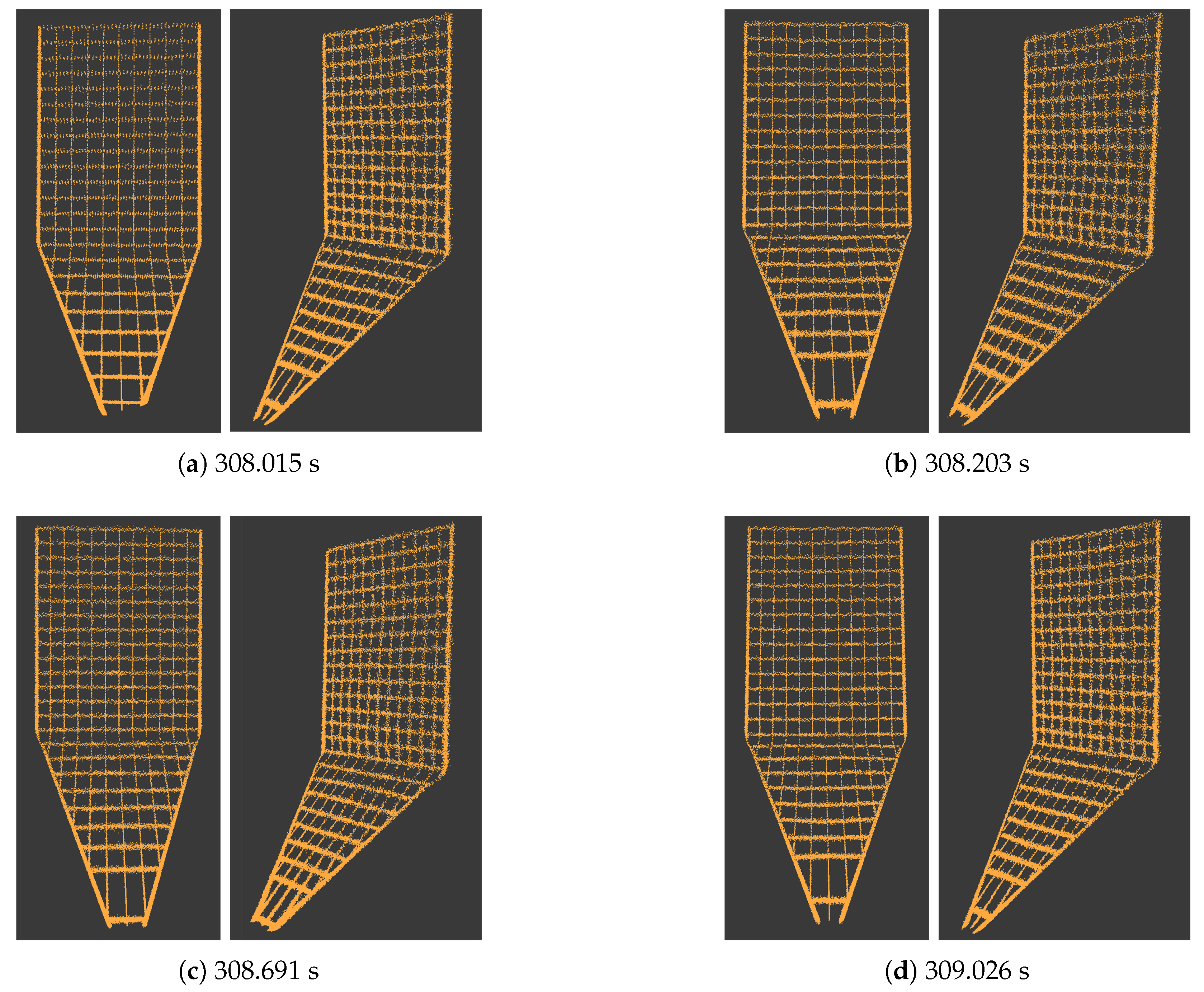
In order to estimate the true value of dynamic parameters, it is necessary to estimate the real-time position of the nodes at first. The estimation results of the four moments after collision are shown in Figure 14 and Table 8. It can be seen that the estimation results of the nodes after collision are good, with the average position errors less than 5.2% and the single calculation time less than 0.06 s, which proves that it can provide a good data basis for the subsequent estimation of the true value of mass and principal moment of inertia.
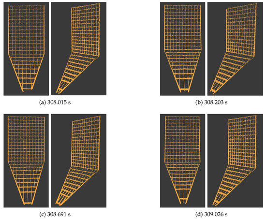
Figure 14.
Identification of the rope net nodes.
Table 8.
Simulation results: statistical results of node calculation errors.
Then, the mass and angular momentum parameters are identified by using the identified node positions of the rope net. The results are shown in Figure 15a,b. It can be seen that the identification error of debris mass is less than 0.72% after 312.49 s (12.49 s after calculation) and less than 0.59% after 311.26 s (11.26 s after calculation). The relative errors of normalized angular kinetic energy and angular momentum calculated based on the results are less than 2.37%. The simulation results show that the true value of full dynamic parameters of space debris can be obtained after 20 s of actual operation and the relative errors are less than 3%, which proves that this method can provide an accurate data foundation for detumbling capture operation quickly.
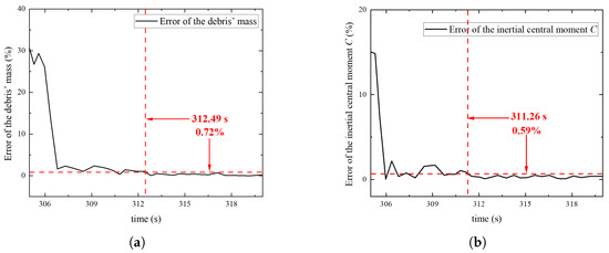
Figure 15.
Simulation results: identification of the true value of inertial parameters. (a) Identification of the mass. (b) Identification of the central principle moment of inertia.
5. Conclusions
In this paper, an efficient method for identifying full dynamic parameters of large space debris by analyzing the collision characteristics based on visual flexible collision with rope mesh is proposed. The method consists of two steps: (1) normalization parameter identification before collision, (2) true value calculation of dynamic parameters after collision. Before the collision, the space debris point cloud is obtained by LiDAR, the motion parameters of the debris are calculated through the point cloud registration, and the real-time position of the debris mass center is optimized by using the motion data and the motion equation of the feature points. Furthermore, through the initial position of center of mass and the point cloud transformation matrix at each moment, the transformation relationship between the LiDAR coordinate system and the debris fixed coordinate system is obtained, and the debris motion data is transferred to the debris fixed coordinate system. Thus, the normalized inertia tensor, normalized kinetic energy and angular momentum direction of the debris are solved based on the debris dynamic model and dynamic parameter characteristics. After the collision, the debris, satellite and rope network are regarded as a whole system, and real-time momentum characteristics of the rope net which are difficult to measure are calculated based on the change in node point cloud position of the rope network. The mass and true value of the main moment of inertia of the debris are calculated by the conservation of linear momentum and angular momentum of the system, and the true value of the kinetic energy and momentum of the debris are obtained after the true value of the moment of inertia is substituted into the normalized parameters. Finally, full dynamic parameters of large space debris are identified. The identification of center of mass and normalized dynamic parameters is performed. The results show that the average error of the initial position of the mass center is less than 0.81%, the average error of the single calculation of mass center is less than 0.5%, the maximum error is less than 1.3% and the calculation time is less than 0.17 s. When the actual identification time reaches 1.68 s, the deviation of the normalized principal moment of inertia converges to less than 0.96%. The error of normalized angular kinetic energy converges to less than 1.2% after 2.67 s (the actual identification time). When the actual identification time reaches 2.17 s, the error of normalized angular momentum converges to less than 1.2%; meanwhile, when the actual identification time reaches 3.77 s, the triaxial error of angular momentum direction is all less than 0.61%. After the debris collides, the simulation of identifying the true value of the dynamic parameters is carried out. The average position calculation error of the nodes is less than 5.2%, and the single calculation time is less than 0.06 s. The identification error of debris mass is less than 0.72% after 12.49 s and the identification error of the inertial central moment less than 0.59% after 11.26 s. The relative errors are less than 2.37% after substituting the inertial central moment into the normalized angular kinetic energy and angular momentum values. The simulation results show that all the dynamic parameters of space debris can be obtained after 20 s of actual operation and the relative errors are less than 3%, which proves that our method is more in line with the actual needs of detumbling and capture mission.
In this paper, we adopted the conservation of momentum before and after debris collision to achieve a high-precision solution of the real values of the dynamic parameters of large space debris. However, due to the time consuming solving of the point cloud transformation matrix, 300 s of point cloud data sampling is required before identification to achieve a relatively high-precision parameter solution. Subsequently, we will carry out research on a point cloud registration algorithm based on the debris motion characteristics of space debris and the characteristics of point cloud data, so as to improve the solving efficiency of the high-point cloud transformation matrix and further improve the identification effect of the dynamic parameters of large space debris.
Author Contributions
Methodology, C.W.; formal analysis, C.T.; investigation and writing—original draft preparation, H.Z.; writing—review and editing, C.T., J.Y. and L.L.; supervision, Y.Z. All authors have read and agreed to the published version of the manuscript.
Funding
This work was financially supported by the National Natural Science Foundation of China (Number U21B2075) and the Stable Supporting Fund of National Key Laboratory of Underwater Acoustic Technology (JCKYS2023604SSJS012).
Data Availability Statement
Data are unavailable due to privacy or ethical restrictions.
Acknowledgments
Thanks to the Harbin Institute of Technology and Harbin Engineering University for their financial and equipment support for this project.
Conflicts of Interest
The authors declare no conflict of interest.
References
- Tao, J.; Cao, Y.; Ding, M. Progress of Space Debris Detection Technology. Laser Optoelectron. Prog. 2022, 59, 1415010. [Google Scholar]
- Sun, C.; Wan, W.; Deng, L. Adaptive space debris capture approach based on origami principle. Int. J. Adv. Robot. Syst. 2019, 16, 1729881419885219. [Google Scholar] [CrossRef]
- Sun, Y.; Wang, Q.; Jiao, R.; Liu, R.; Jin, M. Design of a non-cooperative target capture mechanism for capturing satellite launch adapter ring. Proc. Inst. Mech. Eng. Part J. Aerosp. Eng. 2023, 237, 1060–1077. [Google Scholar] [CrossRef]
- Peng, S.; Zhang, H.; Qi, C.; Xu, J.; Ma, R.; Dai, S. Impact Pressure Distribution Recognition for Large Non-Cooperative Target in Ground Detumbling Experiment. Aerospace 2022, 9, 226. [Google Scholar] [CrossRef]
- Pardini, C.; Anselmo, L. Revisiting the collision risk with cataloged objects for the Iridium and COSMO-SkyMed satellite constellations. ACTA Astronaut. 2017, 134, 23–32. [Google Scholar] [CrossRef]
- Navabi, M.; Hamrah, R. Close approach analysis of space objects and estimation of satellite-debris collision probability. Aircr. Eng. Aerosp. Technol. 2015, 87, 483–492. [Google Scholar] [CrossRef]
- Setterfield, T.P.; Miller, D.W.; Saenz-Otero, A.; Frazzoli, E.; Leonard, J.J. Inertial Properties Estimation of a Passive On-orbit Object Using Polhode Analysis. J. Guid. Control. Dyn. 2018, 41, 2214–2231. [Google Scholar] [CrossRef]
- Setterfield, T.P.; Miller, D.W.; Leonard, J.J.; Saenz-Otero, A. Mapping and determining the center of mass of a rotating object using a moving observer. Int. J. Robot. Res. 2018, 37, 83–103. [Google Scholar] [CrossRef]
- Setterfield, T.P. On-Orbit Inspection of a Rotating Object Using a Moving Observer; Massachusetts Institute of Technology: Cambridge, MA, USA, 2017. [Google Scholar]
- Tweddle, B.E.; Setterfield, T.P.; Saenz-Otero, A.; Miller, D.W. An Open Research Facility for Vision-Based Navigation Onboard the International Space Station. J. Field Robot. 2016, 33, 157–186. [Google Scholar] [CrossRef]
- Tweddle, B.E. Computer Vision-Based Localization and Mapping of an Unknown, Uncooperative and Spinning Target for Spacecraft Proximity Operations; Massachusetts Institute of Technology: Cambridge, MA, USA, 2013. [Google Scholar]
- Tweddle, B.E.; Saenz-Otero, A.; Leonard, J.J.; Miller, D.W. Factor Graph Modeling of Rigid-body Dynamics for Localization, Mapping, and Parameter Estimation of a Spinning Object in Space. J. Field Robot. 2015, 32, 897–933. [Google Scholar] [CrossRef]
- Yao, J.; Liu, Y.; Zhang, H.; Dai, S. Dynamic Parameter Estimation of Large Space Debris Based on Inertial and Visual Data Fusion. Actuators 2021, 10, 149. [Google Scholar] [CrossRef]
- Che, D.; Zheng, Z.; Yuan, J. An Innovate Detumbling Method for a Non-Cooperative Space Target via Repeated Tentative Contacts. IEEE Access 2022, 10, 64435–64450. [Google Scholar] [CrossRef]
- Bourabah, D.; Field, L.; Botta, E.M. An Impact Pressure Distribution Recognition for Large Non-Cooperative Target in Ground Detumbling Experiment. ACTA Astronaut. 2023, 202, 909–926. [Google Scholar] [CrossRef]
- Chu, Z.; Ma, Y.; Hou, Y.; Wang, F. Inertial parameter identification using contact force information for an unknown object captured by a space manipulator. ACTA Astronaut. 2023, 131, 69–82. [Google Scholar] [CrossRef]
- Meng, Q.; Liang, J.; Ma, O. Identification of all the inertial parameters of a non-cooperative object in orbit. Aerosp. Sci. Technol. 2019, 91, 571–582. [Google Scholar] [CrossRef]
- Meng, Q.; Zhao, C.; Ji, H.; Liang, J. Identify the full inertial parameters of a non-cooperative target with eddy current detumbling. Adv. Space Res. 2020, 66, 1792–1802. [Google Scholar] [CrossRef]
- Stoyanov, T.; Magnusson, M.; Andreasson, H.; Lilienthal, A.J. Fast and accurate scan registration through minimization of the distance between compact 3D NDT representations. Int. J. Robot. Res. 2012, 31, 1377–1393. [Google Scholar] [CrossRef]
- Anz-Meador, P.D.; Opiela, J.; Shoots, D.; Liou, J.C. History of On-Orbit Satellite Fragmentations; NASA/TM-2018-220037; NASA: Washington, DC, USA, 2018.
- Xu, G.; Xu, J. Chapter 4: Perturbations on the Orbits. In Orbits 2nd Order Singularity-Free Solutions; Xu, G., Xu, J., Eds.; Springer: Berlin/Heidelberg, Germany, 2013; pp. 39–68. [Google Scholar]
- Tang, C.; Huang, Z.; Wei, C.; Zhao, Y. Dynamic and sliding mode control of space netted pocket system capturing and attitude maneuver non-cooperative target. Mech. Sci. 2022, 13, 751–760. [Google Scholar] [CrossRef]
- Gu, H.; Gao, H.; Wei, C.; Huang, Z. A dexterous motion control method of rope driven snake manipulator considering the rope-hole properties. Mech. Mach. Theory 2023, 183, 105219. [Google Scholar] [CrossRef]
- Jiang, J.; Wei, C.; Yu, Y.; Sun, S. Autonomous Planning of Discontinuous Terrain-Dependent Crawling for Space Dobby Robots. Sensors 2023, 23, 3334. [Google Scholar] [CrossRef]
- Zhang, Y.; Wei, C.; Zhao, Y.; Tan, C.; Liu, Y. Adaptive ANCF method and its application in planar flexible cables. Acta Mech. Sin. 2018, 34, 199–213. [Google Scholar] [CrossRef]


Disclaimer/Publisher’s Note: The statements, opinions and data contained in all publications are solely those of the individual author(s) and contributor(s) and not of MDPI and/or the editor(s). MDPI and/or the editor(s) disclaim responsibility for any injury to people or property resulting from any ideas, methods, instructions or products referred to in the content. |
© 2023 by the authors. Licensee MDPI, Basel, Switzerland. This article is an open access article distributed under the terms and conditions of the Creative Commons Attribution (CC BY) license (https://creativecommons.org/licenses/by/4.0/).