Research on Magnetic Characteristics and Fuzzy PID Control of Electromagnetic Suspension

Abstract

This paper proposes an electromagnetic suspension with an electromagnetic actuator, which can improve the riding comfort and stability of the vehicle without changing the safety of traditional MacPherson suspension. First, the electromagnetic suspension structure is introduced, and the principle of the proposed actuator is described in detail. Second, a magnetic flux density model of a single PM ring (permanent magnetic ring) and a magnet assembly are built, and a theoretical analysis of the magnetic flux density is carried out for comparison. Then, the magnetic flux distribution of the magnetic field is simulated and analyzed using the finite element method (FEM), and is compared with theoretical and other experimental data. Finally, a vehicle dynamics model with 7 DOF is built, and vehicle simulations based on the fuzzy PID algorithm are carried out on a C-grade road surface and a deceleration strip. The theoretical results and simulation analyses of the FEM indicate that compared with the MacPherson suspension, the root mean square values of the acceleration of centroid acceleration for the electromagnetic suspension are increased by 59.08% and 33.34%, respectively, on a C-grade road surface and a deceleration strip, and other physical quantities have also been improved. The structure and characteristics of the proposed electromagnetic suspension that improve the riding comfort of the suspension and enhance the stability of the MacPherson suspension are feasible.

1. Introduction

The rapid growth in the number of vehicles, driven by the development of transportation and the improvement of people’s quality of life, has attracted increasing attention on body vibration and tire wear. This concerns not only the safety and integrity of the goods transported by automobiles but also the riding comfort and handling stability of the vehicle [1]. As a key component of the vehicle’s body, the chassis not only supports the vehicle but also accepts the thrust generated by the engine, ensuring the normal operation of the vehicle [2,3]. Suspension systems, as key components of automobile chassis, have garnered significant research interest.

Suspension systems play a key role in supporting the vehicle body and ensuring the comfort, stability, and safety of vehicles. The research and development of comprehensive suspension system performance is a key factor affecting vehicle performance, body direction and attitude control, handling stability, and the driving and riding experience. McPherson-independent suspension, widely used in the front suspension of modern cars, has several shortcomings, including small brake resistance, weak suspension stiffness, poor stability, and a noticeable turning roll. Therefore, designing a high-performance automobile suspension system can fundamentally improve the performance of an automobile [4,5]. Suspension systems are developing towards the direction of lighter weight, smaller volume, faster responses, more stable running state, and greater safety and reliability. With the development of cities and increasing road pressure, vehicles, particularly their suspension systems, are more susceptible to problems [6]. The performance of a suspension system mainly depends on the response ability of its actuator or the motor-to-road conditions. Therefore, it is of great significance to research and discuss automobile suspension systems and their related components.

Compared with passive suspension systems, semi-active suspension systems can change the damping of shock absorbers by controlling the input of a single variable so as to adapt to different road conditions [7,8,9]. At present, there are two types of adjustable shock absorbers in semi-active suspension systems, which differ in terms of the amount of control they exert. One adjusts the damping size of the damper solenoid valve by adjusting the effective area of the throttle, but this method cannot avoid suspension system noise and stability and reliability problems. The other adjusts the spring rigidity of the whole shock absorber by changing the spring stiffness of the variable spring, but this may produce bumps during the driving process.

Because there are no components with controllable forces installed in the system, a semi-active suspension system cannot control the stiffness of the spring. Therefore, research on semi-active suspension is greatly limited, and the improvement of vehicle performance when using this suspension type is also greatly limited [10].

In recent years, researchers have designed various active suspension systems, including those with rack and pinion rotating motors [11,12,13,14], ball screw mechanisms [15,16,17,18], hydraulic actuating quarter-car active suspension systems [19], and electromagnetic suspension [20,21,22], among others. With the development of electromagnetic control technology and PM material, electromagnetic suspension as a new type of suspension structure has become of interest for researchers, such as traditional hydraulic dampers with a linear motor [23], mechanisms with a ball screw mechanism and two one-way clutches [24], coreless linear tube actuators with a special topology [25,26], electromagnetic and hydraulic suspensions [27], and rotating semi-active electromagnetic variable stiffness devices [28], and so on. They use these mechanisms instead of the dampers or springs of traditional suspensions, or even both can be used. However, safety was not considered in the event of suspension failure or power failure.

Suspension using a motor, magnetorheological fluid damper [29,30], and suspension using an electromagnetic actuator are examples of active electromagnetic suspension. Compared with the first two types of active suspension, electromagnetic actuator suspension is simpler and more efficient in terms of its structure, performance, magnetic force, processing, and so on. An electromagnetic actuator can greatly improve the reaction speed of a suspension system, and thus, it has become the research focus of more and more scholars [31,32]. In addition, electromagnetic actuators also have the advantages of simple system configuration, fast response speed, and energy recycling, and as a result, they are more and more widely used.

Integrating control methods into active suspension systems can significantly enhance their performance. In [33], the semi-active suspension of automotive magnetorheological fluids was controlled by a fuzzy control algorithm, and the overall performance of the suspension was improved. In [34], a semi-active 1/4 suspension with three degrees of freedom utilizing a magneto-rheological shock absorber was controlled by a hybrid fuzzy and fuzzy PID controller. In [35], a fuzzy PID controller was applied in a half vehicle active suspension system to enhance the vibration levels of the vehicle chassis and passenger seat. Therefore, the fuzzy PID control algorithm combines the advantages of fuzzy control and PID control, which makes it suitable for research on controlling electromagnetic suspension.

This paper aims to make up for the ride comfort and stability of the vehicle without changing the safety of the McPherson suspension. In this paper, we propose an electromagnetic suspension structure that can improve the stability and ride comfort performance of vehicles and make up for the defects of the McPherson suspension. Firstly, the structure of the proposed suspension is introduced, and its principle is described in detail. Secondly, the magnetic flux density model of a single PM ring and a magnet component is established, and the theoretical analysis of the magnetic flux density is carried out. Then, the magnetic flux distribution of the magnetic field is analyzed via the two-dimensional finite element method, and the magnetic flux density is simulated via finite element analysis. Finally, a vehicle dynamics model with seven degrees of freedom is established, and a vehicle simulation on C-grade roads and a deceleration strip is carried out based on the fuzzy PID algorithm. After improving the MacPherson suspension system, active control, four-wheel ride comfort, and stability issues were studied with C-grade roads and a deceleration strip.

2. Structure and Principle

The proposed structure of the electromagnetic actuator uses a 1/4 MacPherson-type independent suspension system, as shown in Figure 1a. The electromagnetic actuator is inserted into the gap between the hydraulic damper and the spring, the coil assembly of the electromagnetic actuator is connected with the upper cover, and the magnet assembly of the electromagnetic actuator is connected with the cylinder tube of the hydraulic damper, as shown in Figure 1b. The spring, electromagnetic actuator, and hydraulic damper are connected in parallel. The magnet assembly adopts a double-layer PM magnet ring form, and the coil assembly moves in the air gap of the magnet assembly. Compared to the magnet assembly, the coil weighs less; the coils are connected to the upper cover of the shock absorber, which facilitates connection to the vehicle’s internal circuit. Consequently, the electromagnetic suspension can be controlled by inputting a current to resolve the disadvantages of the MacPherson-type independent suspension. In this application, it is necessary to maintain a safe distance between the electromagnetic actuator and the spring. When the spring compresses to its lowest point, the distance between the upper cover and lower cover is longer than the axial distance of the electromagnetic actuator, which means that it can avoid the strike of the upper cover and the lower cover at the compression limit. A characteristic of this electromagnetic suspension is that it does not change the structure of the MacPherson suspension. It not only ensures the safety of the MacPherson suspension, but it also improves the stability of the MacPherson suspension.

The structure of the proposed electromagnetic actuator is shown in Figure 2. The coil assembly involves a group of coils moving along the axis of the actuator. The magnet assembly consists of the outer wall, six small PM rings, and six large PM rings for radial magnetization, heat-dissipated rings, and a fixed plug. Each PM ring is composed of eight identical pieces, and their material is Nd–Fe–B, and the PM rings are magnetized inside as the S pole and the outside as the N pole. The outer wall and the fixed plug are used to fix the PM rings. The heat-dissipated ring is used for dissipating heat between two PM rings to avoid the phenomenon of heat accumulation. The fixed plug plays a role in fixing the PM rings and heat-dissipated rings. Large PM rings and small PM rings are placed side by side; the magnet assembly can generate a quasi-parallel magnetic field.

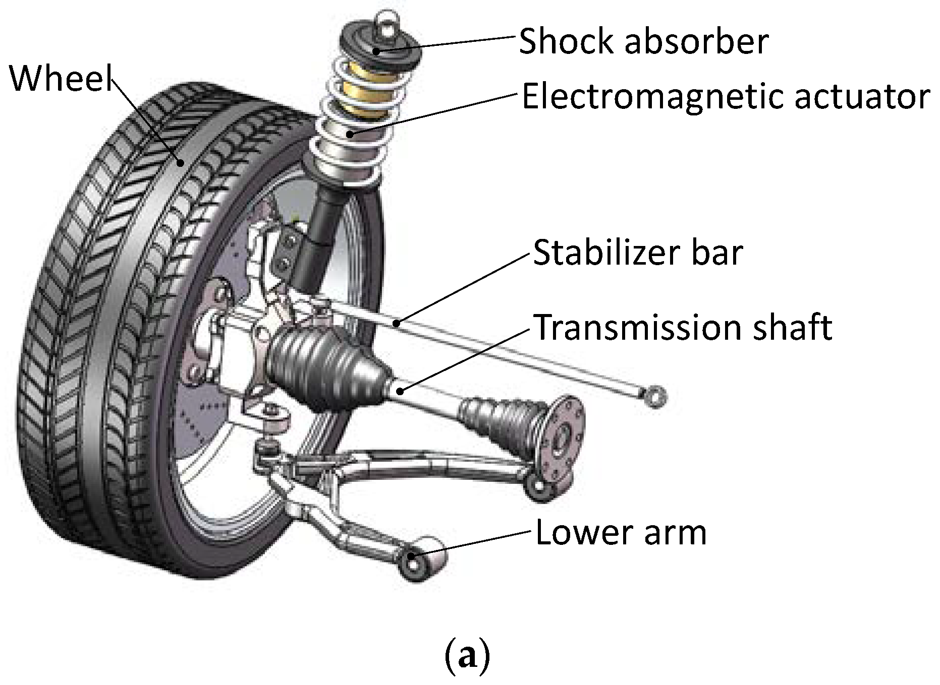
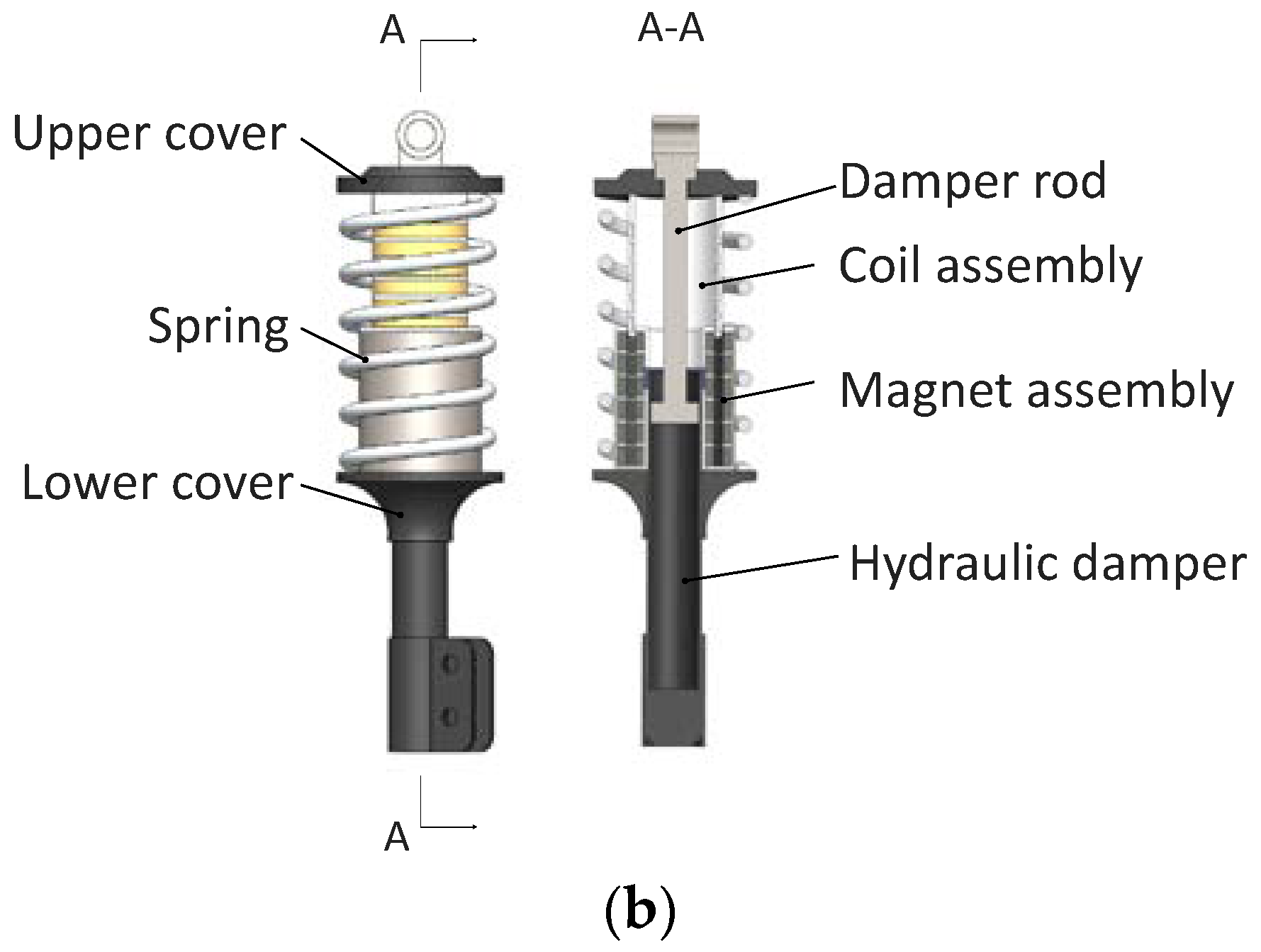
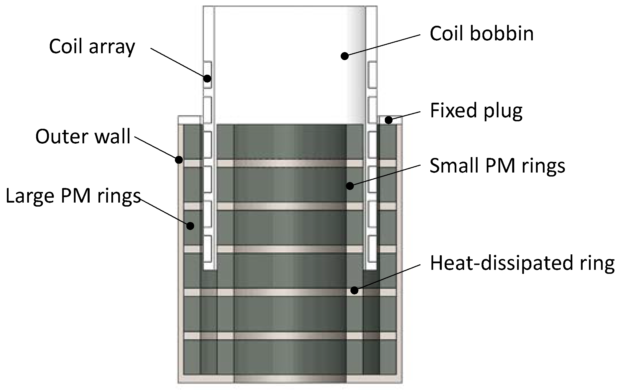
2.1. Design of the Electromagnetic Actuator

For electromagnetic actuators, it is necessary to achieve a compact size and a large magnetic force. The influence of the height and radial length of large/small PM rings and the height of coils on the magnetic force of the proposed actuator was analyzed using orthogonal experimental methods. As shown in

Table 1. Factors and levels in the orthogonal experiment method.

Level	Height of Large/Small PM Rings (mm) A	Radial Length of Large/Small PM Rings (mm) B	Height of Coils (mm) C
1	10.5	10	5.5
2	11.5	11	9.5
3	12.5	12	12.5

, height and radial length of large/small PM rings and the height of coils were determined as three factors for the orthogonal experimental method, with each factor having three levels. The simulation parameters are that the coercivity of the PM ring is 868 KA/m and the residual magnetic flux density of the PM ring is 1.38–1.44 T. The L₉ (3² × 3²) size optimization simulations of the actuator by the orthogonal experiment method are shown in

Table 2. L₉ (3² × 3²) size optimization simulations of the actuator by the orthogonal experiment method.

Number	Height of Large/Small PM Rings (mm)	Radial Length of Large/Small PM Rings (mm)	Height of Coils (mm)	Magnetic Force (N)
1	A1	B1	C1	156
2	A1	B2	C2	171
3	A1	B3	C3	156
4	A2	B1	C2	135
5	A2	B2	C3	159
6	A2	B3	C1	171
7	A3	B1	C3	165
8	A3	B2	C1	150
9	A3	B3	C2	180

.

The analysis by the orthogonal experiment method (L₉ (3² × 3²) size) is shown in

Table 3. Analysis by the orthogonal experiment method.

Value Name	Height of Coil2 (mm)	Thickness of Coil2 (mm)	Height of Soft Iron Ring1 (mm)
Kj1	543	516	537
Kj2	525	540	546
Kj3	555	567	540
Kjp1	181	172	179
Kjp2	175	180	182
Kjp3	185	189	180
Rj	10	17	3
Primary and secondary order	B > A > C
Optimal levels	A3	B3	C2
Optimal combination	A3B3C2

Note: K_jk (k = 1, 2, 3) is the sum of the simulation results with the same level k in the j^th column. K_jpk is the mean value of the simulation results with the same level k in the j^th column. R_j is the range of K_jpk.

. As can be observed, the combination (A3B3C2) is the optimal parameters, which are the height of large/small PM rings (12.5 mm), the radial length of large/small PM rings (12 mm), and the height of coils (9.5 mm).

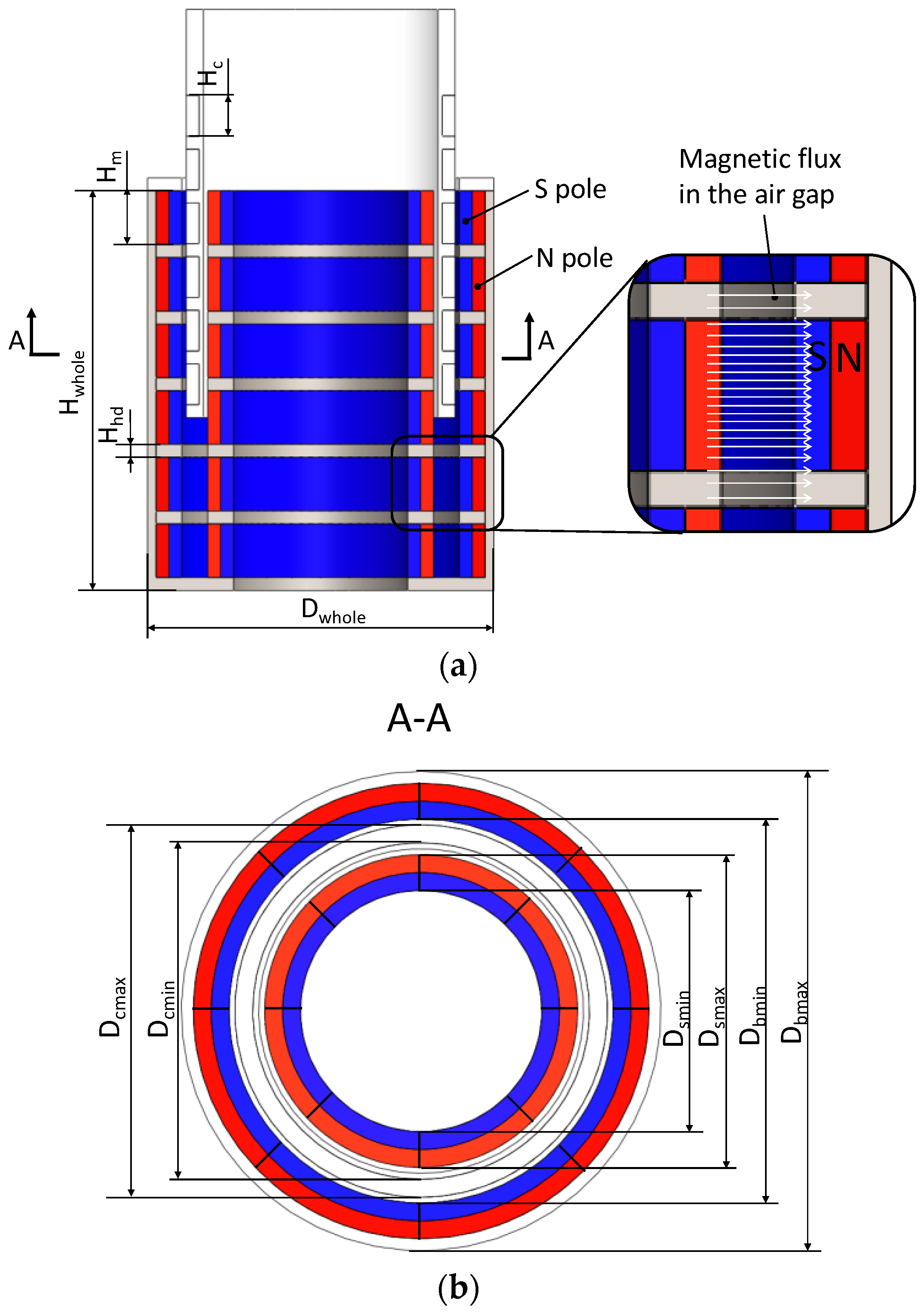
2.2. Sizes and Principles of the Electromagnetic Actuator

According to Section 2.1, the dimension mark and magnetic flux in the air gap are as shown in Figure 3. Figure 3a,b, respectively, show sectional views in the radial direction and in the axial direction. The magnetic flux is emitted from the N pole of the small PM rings through the air gap, the coils, and the coil bobbin. Then, it is gathered at the S level of the large PM ring. This structure for dual PM rings can generate magnetic flux in the same direction as the air gap, which is equivalent to increasing the magnetic focusing effect. Six groups of the dual PM rings generate magnetic flux in the same direction within the air gap. When the coils move in the axial direction, they cause as much magnetic flux as possible. The size parameters of the electromagnetic actuator are shown in

Table 4. Size parameters of the electromagnetic actuator.

Size Parameter	Description	Value (Unit: mm)
Hc	Axial length of the coils	9.5
Hm	Axial length of the PM ring	12.5
Hhd	Axial length of the heat-dissipated ring	3
Hwhole	Axial length of the actuator	96
Dwhole	Outside diameter of the actuator	80.6
Dcmax	Outside diameter of the coils	62.3
Dcmin	Inside diameter of the coils	56.6
Dsmax	Outside diameter of the small PM rings	52.6
Dsmin	Inside diameter of the small PM rings	40.6
Dbmax	Outside diameter of the large PM rings	76.6
Dbmin	Inside diameter of the large PM rings	64.6

.

3. Model and Analysis of the Magnetic Field

In the electromagnetic actuator, the magnetic field in the air gap of the stator is the main factor for improving performance. The homogeneity of the magnetic field in the air gap along the actuator’s axial direction decides the stability and linearity of the actuator’s thrust force. The magnetic flux density in the air gap decides the thrust force of an actuator and the ride comfort of a vehicle. First, the model of the magnetic flux density in an air gap is built, and the characteristic of the magnetic field is theoretically analyzed.

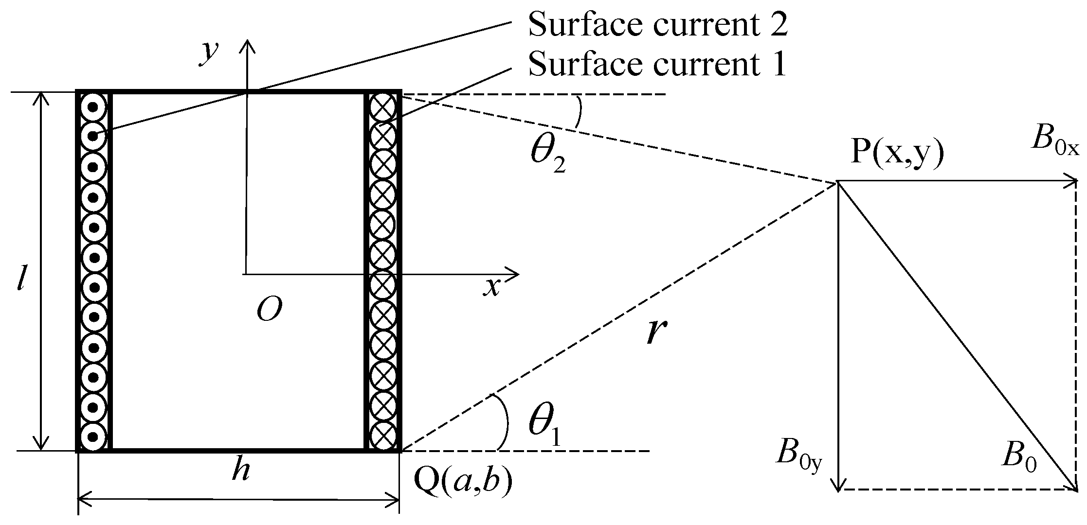
3.1. Magnetic Flux Density Model of a Single PM Ring

To analyze the quasi-parallel magnetic field in the air gap between the PM ring arrays and the inner wall of the actuator, the mathematical model of the magnetic flux density of the magnet field is built in the y direction according to the Ampere molecular circulation hypothesis, as shown in Figure 4. When the positive direction of the magnet field is +y direction, the spatial magnetic field is equivalent to the magnetic field generated by Surface Currents 1 and 2 [36,37].

A schematic diagram of the magnetic field of a single PM ring is shown in Figure 4. The description of the variables in the formulas is shown in

Table 5. Variable table.

Variable	Description
Q(a, b)	Horizontal and vertical coordinates of any current source
P(x, y)	Horizontal and vertical coordinates of any point in a plane
j	Ring number from left to right, j = 1–6
θ1, θ2	Angle between the upper and lower points of surface current 1
θ	Angle between the line of point Q and point P and the horizontal line
r	Distance between point Q and point P
Byj1	Magnetic flux density of surface current 1
Byj2	Magnetic flux density of surface current 2
By1	Magnetic flux density of large PM rings
By2	Magnetic flux density of small PM rings
By	Magnetic flux density of the PM ring array

. The magnetic flux density formula at point P(x, y) in the y direction can be expressed as follows [38,39,40]:

$$B_{\mathrm{oy}}=-B_o\cos \theta$$

(1)

where

$$B_{\mathrm{o}}=\frac{{\mu }_0{k}_{\mathrm{v}}}{2\mathsf{\pi }r};\theta =\arcsin (\frac{y-b}{r})$$

The magnetic flux density B_y11 and B_y12 generated by the surface currents 1 and 2 can be expressed as (2) and (3) [41,42,43]:

$$\begin{array}{ll}{B}_{y11}& ={\displaystyle {\int }_{{\theta }_1}^{{\theta }_2}\frac{{\mu }_0{k}_v}{2\mathsf{\pi }r}}\sin \theta \mathrm{d}b\\ & =\frac{{\mu }_0{k}_v}{2\mathsf{\pi }}[\arctan (\frac{y-l/2}{x-h/2})-\arctan (\frac{y+l/2}{x-h/2})]\end{array}$$

(2)

$$\begin{array}{ll}{B}_{y12}& =-{\displaystyle {\int }_{{\theta }_1}^{{\theta }_2}\frac{{\mu }_0{k}_v}{2\mathsf{\pi }r}}\cos \theta \mathrm{d}b\\ & =\frac{{\mu }_0{k}_v}{2\mathsf{\pi }}[\arctan (\frac{y+l/2}{x+h/2})-\arctan (\frac{y-l/2}{x+h/2})]\end{array}$$

(3)

where

$$\begin{array}{ll}r=\frac{x-h/2}{\cos \theta }& db=-\frac{x-h/2}{{\left(\cos \theta \right)}^2}d\theta \\ {\theta }_1=\arctan (\frac{y+l/2}{x-h/2})& {\theta }_2=\arctan (\frac{y-l/2}{x-h/2})\end{array}$$

3.2. Magnetic Flux Density Model of the Magnet Assembly

To analyze the magnetic fields of two groups of PM ring arrays, the magnetic flux density of the PM ring array B_y in the air gap can be expressed as (4) [43]:

$$\begin{array}{l}{B}_y=B_{y1}+B_{y2}\\ B_y{}_j={\displaystyle \sum _{i=1}^6{B}_{yj1}+}{\displaystyle \sum _{i=1}^6{B}_{yj2}}\end{array}$$

(4)

$$B_{yj1}=\frac{{\mu }_0{k}_v}{2\pi }\arctan (\frac{y-l/2}{x-(j-1)·(h+s)-h/2})-\frac{{\mu }_0{k}_v}{2\pi }\arctan (\frac{y+l/2}{x-(j-1)·(h+s)-h/2})$$

(5)

$$B_{yj2}=\frac{{\mu }_0{k}_v}{2\pi }\arctan (\frac{y+l/2}{x-(j-1)·(h+s)+h/2})-\frac{{\mu }_0{k}_v}{2\pi }\arctan (\frac{y-l/2}{x-(j-1)·(h+s)+h/2})$$

(6)

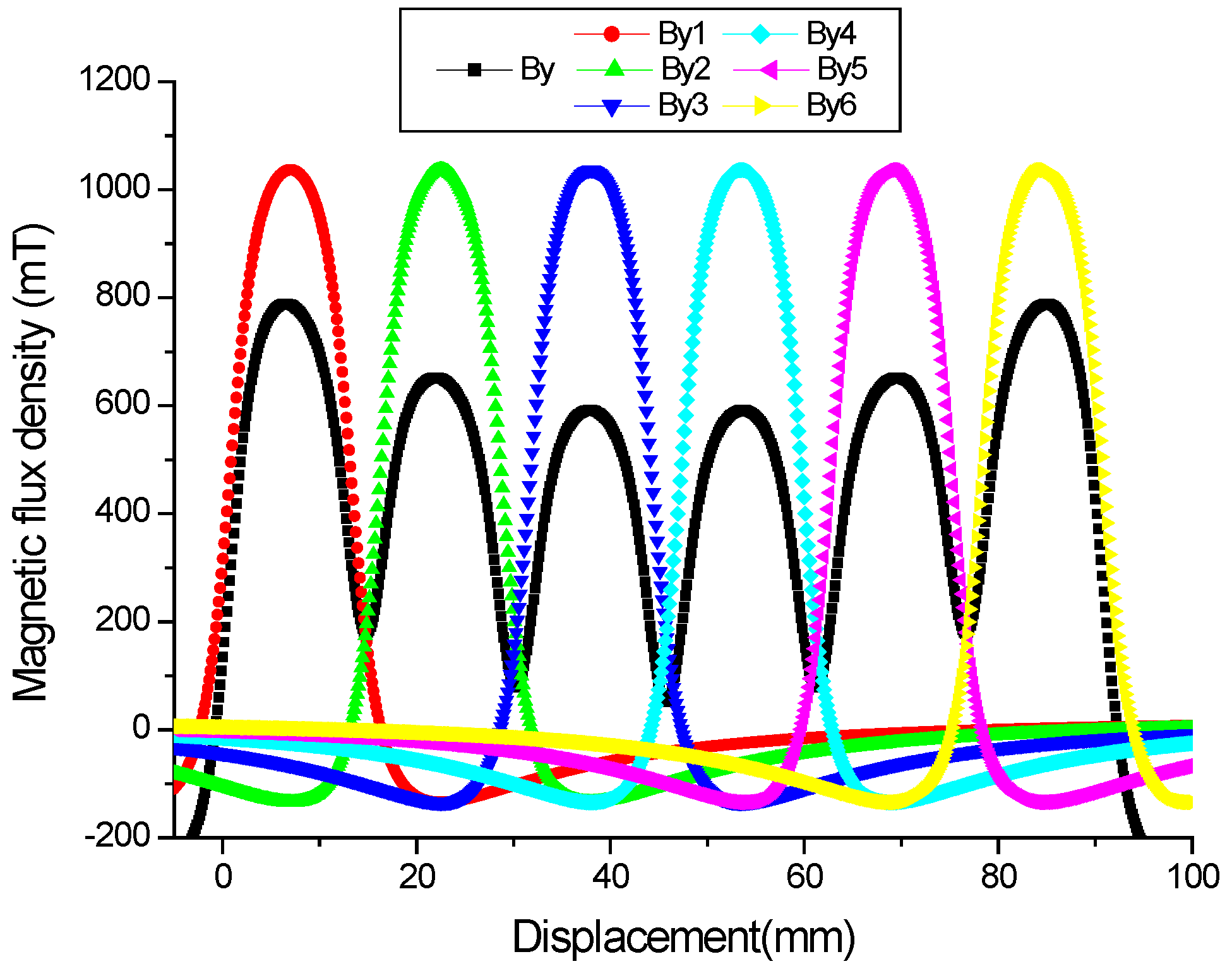
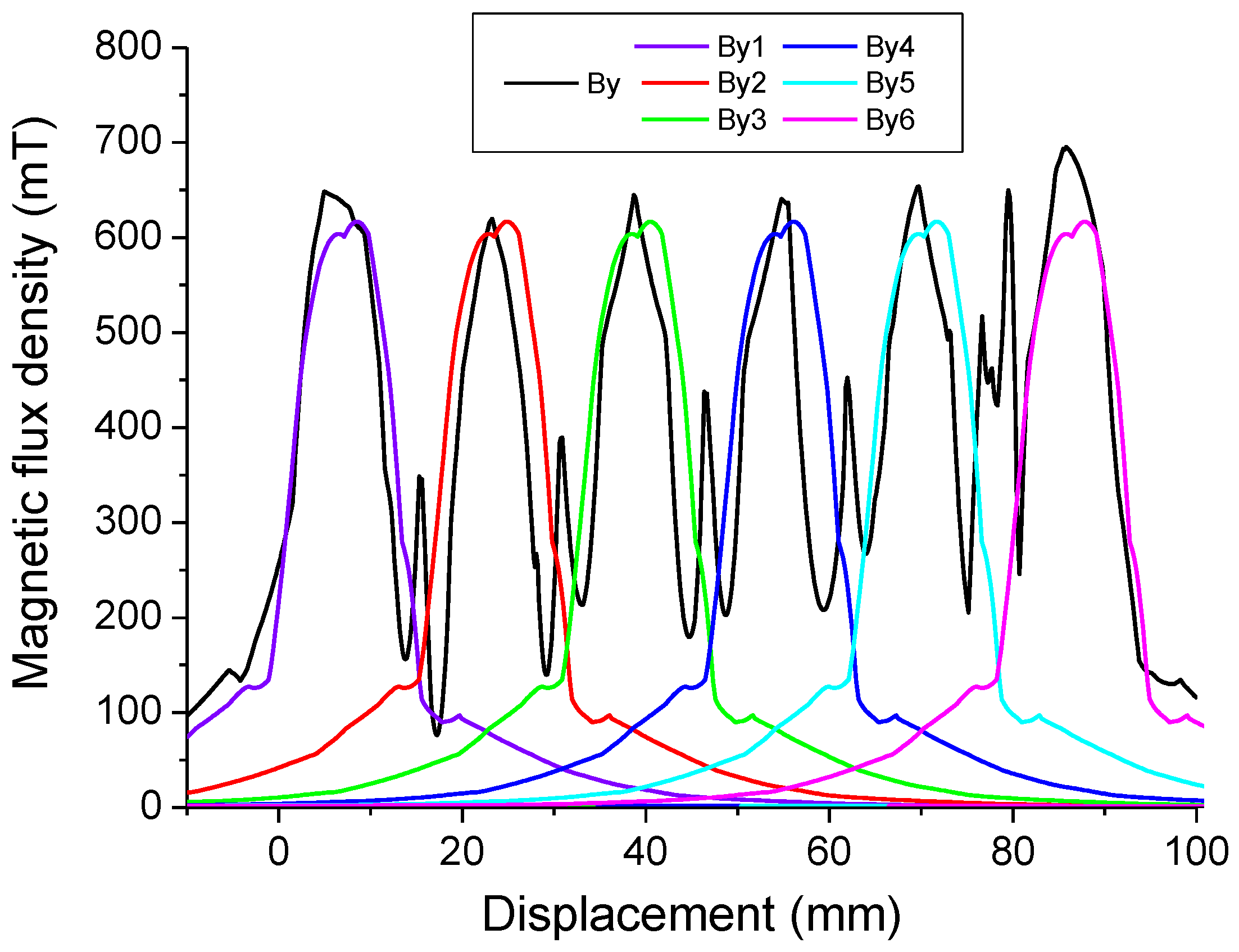
3.3. Theoretical Analysis of Magnetic Flux Density

According to the magnetic flux density model of the actuator’s magnet assembly, the magnetic flux density was calculated by (4) in the middle of the air gap and along the whole axial length of 90 mm. The calculated results of the magnetic flux density of each PM ring and the superimposed magnetic flux density of the six PM ring arrays are shown in Figure 5. The results of each PM ring are shown as a normal distribution curve, the superimposed magnetic flux density B_y is shown as regular fluctuations, and its value varies between 51.73 and 788.49 mT.

4. FEM Analysis of the Magnetic Field

4.1. FEM Analysis Model

To compare with the magnetic field theory model, a 2-D FEM analysis on the magnetic field and magnetic flux density was conducted using a magnetic field analysis software program. A half 2-D FEM model was built with the same dimension parameters as in Table 4, since the structure of the actuator is axisymmetric. In the FEM model, the remanence Br of the permanent magnet was 1.38–1.44 T, and the coercivity was −876 KA/m.

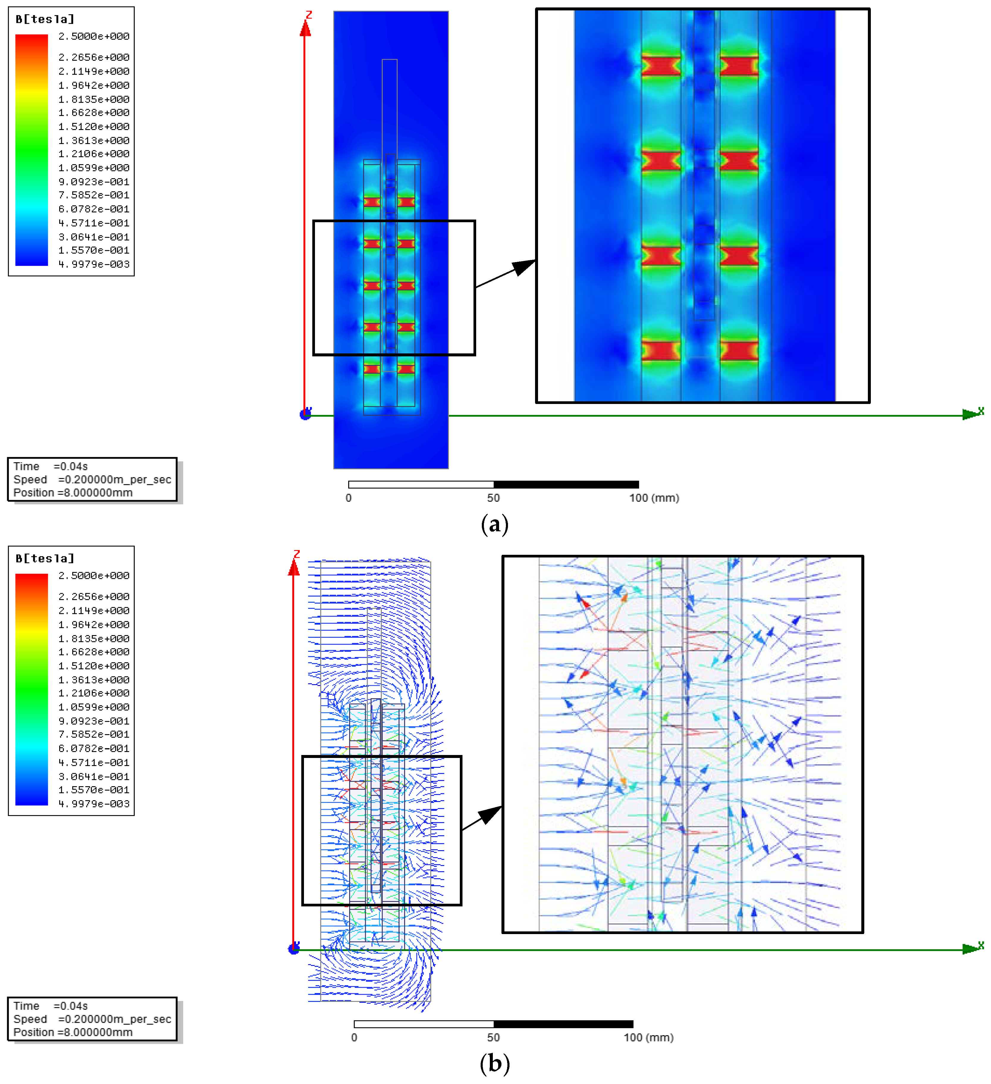
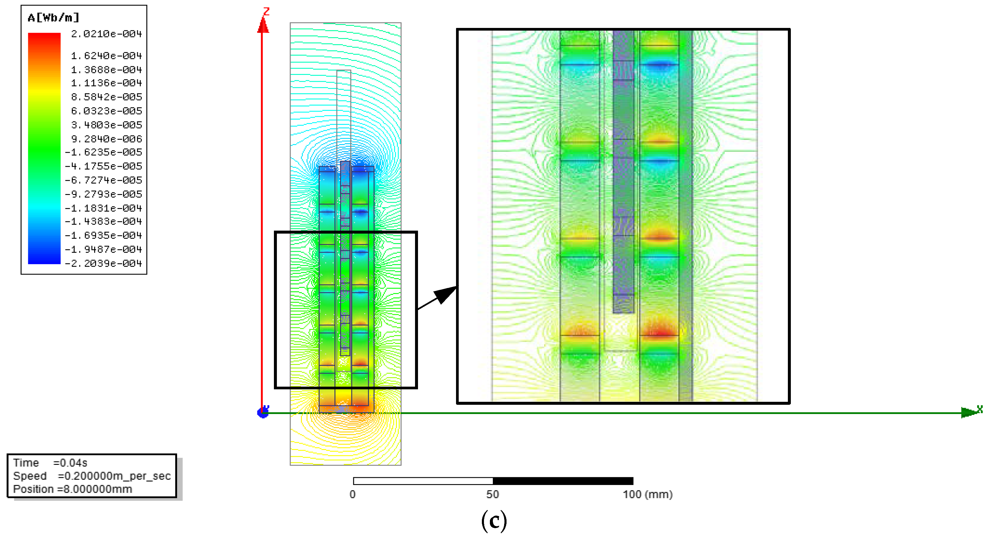
4.2. FEM Analysis on the Magnetic Field

Based on the cylinder coordinate system, the electromagnetic actuator is simulated to obtain the magnetic density and magnetic flux trend by FEM. The simulation adopts a cylindrical coordinate system. The axle of the actuator is z-axis, shown in Figure 6, and the same graphical scales of 0–100 mm are used. The result of the FEM analysis clarifies the characteristics of the quasi-parallel magnetic field for the actuator using PM ring arrays. Since the S pole of the large PM rings is parallel to the N pole of the small PM rings in the air gap of the electromagnetic actuator, there is less magnetic flux leakage. The magnetic flux is nearly parallel in the air gap and its distribution is relatively even in the air gap except for the two ends. This proves that when it moves in the air gap, the coil moves through, cutting the parallel magnetic flux.

Assumption: Each coil has a diameter of 1 mm and a current of 0.8 A is applied. After applying direct current to each coil, the eddy current loss in the simulation is approximately 3 W. Figure 6 shows the simulation structure of the electromagnetic actuator at 0.04 s.

Figure 6a shows the FEM simulation results for the magnetic flux density. From the legend on the left, the magnetic flux density ranges from 4.9979 × 10⁻³ T to 2.500 T. From the magnetic flux density results in the radial direction, it can be seen that the magnetic flux density in the air gap between the large PM rings and the small PM rings is about 550 mT, and the magnetic flux density at both ends is about 670 mT. The magnetic flux density of the large and small heat-dissipated rings is about 1.9 T. The magnetic flux density of the heat-dissipated rings in the middle of the same-size PM rings in the axial direction is relatively large.

Figure 6b shows the FEM simulation results in the direction of magnetic flux. From the legend on the left, the magnetic flux density for the direction of magnetic flux ranges from 4.9979 × 10⁻³ T to 2.500 T, which is the same as in Figure 6a. The results show that the magnetic flux between the large PM rings and the small PM rings is perpendicular to the axial direction of the electromagnetic actuator, and the directions of the multiple magnetic fluxes are parallel to each other. There will be divergence at the edge of each PM ring. Therefore, a magnetic field will be generated at the heat-dissipated rings. In theoretical calculations, the edge effects of the PM rings are assumed to be 0 mT, and this is reflected in the FEM simulation.

Figure 6c shows the FEM simulation results of the magnetic flux trend. From the legend on the left, the magnetic flux distribution for the magnetic flux trend ranges from −2.214 × 10⁻⁴ T to 2.024 × 10⁻⁴ T. The results show that the parallel magnetic field between the large PM rings and the small PM rings is visible, and the magnetic flux in the large heat-dissipated rings and the small heat-dissipated rings is repulsive; in the simulation boundary, due to the inevitable phenomenon of magnetic leakage, the magnetic flux must exist outside the electromagnetic actuator.

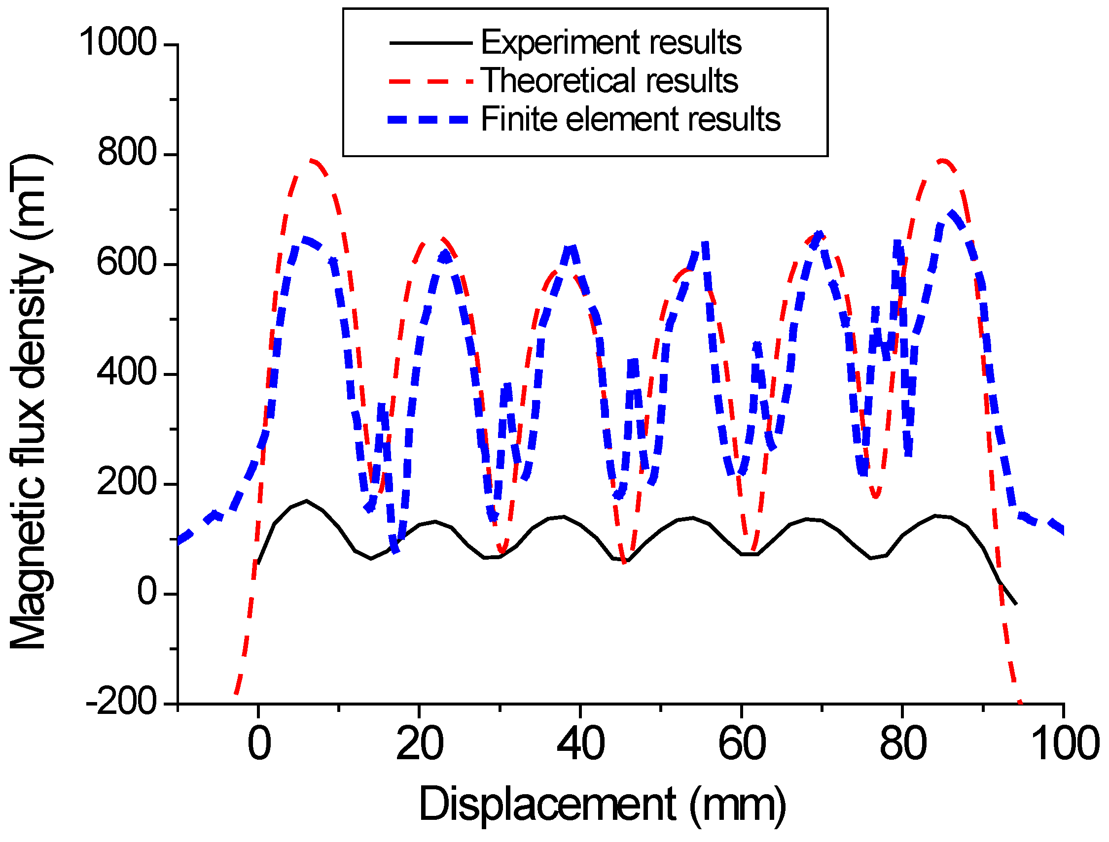
4.3. FEM Analysis of the Magnetic Flux Density

To compare with the theoretical results of the magnetic field model, the superimposed magnetic flux density of the magnet assembly was also analyzed using the 2-D FEM model. The FEM analysis results in Figure 7 clarify the characteristics of the quasi-parallel magnetic field for the magnet assembly using PM ring arrays. The positions of the axial air gap of the PM ring arrays were analyzed, which is the same as the theoretical calculation positions.

Curve By is the magnetic flux density of the PM ring arrays in the axial air gap. Curve By1 to curve By6 are the magnetic flux densities of six magnetic rings from the lower to upper cover. In an air gap magnetic field, the magnetic flux density is roughly in the range of 100 mT–650 mT. Compared to the theoretical result curves, these curves roughly exhibit an irregular sinusoidal shape. At the axial center of the permanent magnet, the magnetic flux density is the highest. At the axial center of the heat-dissipation ring, the magnetic flux density is the smallest. The theoretical calculation curve trend is consistent with the FEM simulation curve trend, with a slightly lower peak magnetic flux density at the middle magnetic rings. The irregular shape of the curve may be due to the consideration of eddy current losses, edge effects of magnets, and other factors in the FEM simulation.

To verify the curve trend of theoretical results and finite element results, the PM arrangement in [44] is similar to that used in this paper. Reference [44] studied an electromagnetic actuator for an active suspension (as shown in Figure 3 of [44]), which uses a single-layer magnetic ring array. The arrangement of magnetic poles is that the outer side is N pole, the inner side is S pole, and each magnetic ring is composed of eight same pieces. The magnetic flux (as shown in Figure 3 of [44]) is emitted from the N pole of the PM rings, passes through the air gap, the outer and inner walls, and then returns to the S pole of the PM rings. This paper adopts a double-layer magnetic ring array, in which the N poles of the small magnetic rings are in face of the S poles of the large magnetic rings in the air gap. Each magnetic ring is also composed of eight same pieces.

In the air gap, compared with the magnet ring array (as shown in Figure 6 of [44]), adding a layer of magnetic ring array will increase the magnetic flux density of the air gap. The theoretical and finite element results of the magnetic ring array are compared and analyzed with the experimental results, as shown in Figure 8. The magnetic field trends of the three curves are consistent, and each curve owns six peaks at the same position. This can prove the correctness of the magnetic flux density trend of the theoretical model derived in this paper. Due to the same position of six peaks, the magnetic flux density will increase as the volume of the magnet rings increases. The experimental results of magnetic field density in [44] are approximately in the range of 50–200 mT, and the theoretical and simulation results of magnetic field intensity in this paper are approximately in the range of 100–650 mT. Therefore, the arrangement of the magnet ring array in this paper with a large magnetic flux density in the air gap is superior to that in [44].

4.4. FEM Analysis on Magnetic Force

Based on the magnetic field characteristics of the electromagnetic actuator, it is necessary to analyze the magnetic force characteristics of the electromagnetic actuator, as shown in Figure 9. The magnetic force characteristics are divided into the current–magnetic force characteristics and the displacement–magnetic force characteristics.

The current–magnetic force curve is shown in Figure 9a. The current range is −1.8 A to 1.8 A, and the magnetic force range of the electromagnetic actuator is −219.8 N to 220.9 N. The current–magnetic force characteristic curve passes through the origin [0,0]. When the current is 1 A, the magnetic force is 122.2 N. When the current is −1 A, the magnetic force is −122.0 N. The slope of the current force curve is approximately 122.2.

The displacement–magnetic force curve is shown in Figure 9b, which is the displacement–magnetic force curve when the current is 0.5 A, 1.0 A, and 1.5 A, respectively. With increasing displacement, the magnetic attenuation is 0.187 N/mm. When the current is 1.0 A and 1.5 A, the magnetic attenuation is 0.376 N/mm and 0.618 N/mm, respectively.

5. Vehicle Simulation Based on the Fuzzy PID Algorithm

To obtain the dynamic characteristics of the electromagnetic suspension, a seven-DOF dynamics model of the whole vehicle was established, and then the fuzzy PID simulation analysis was carried out.

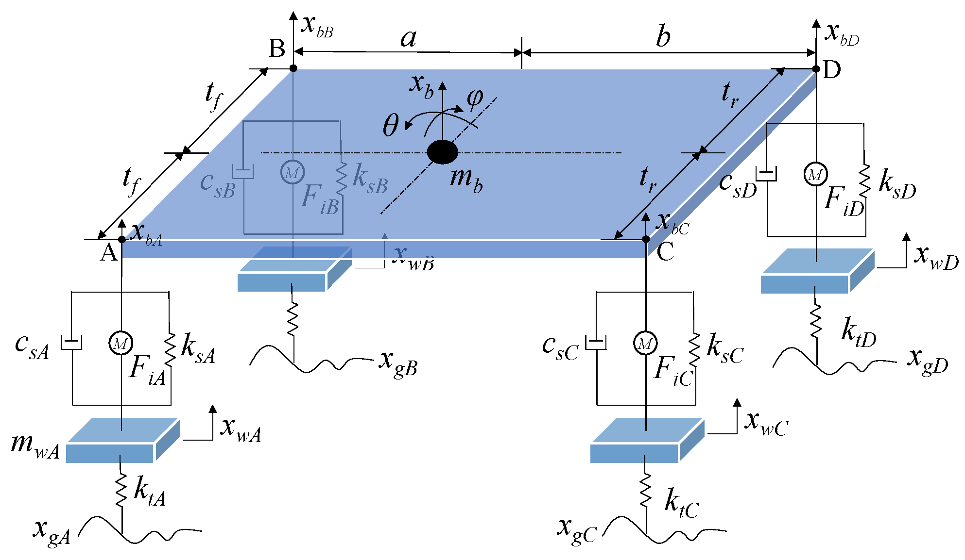
5.1. Vehicle Dynamics Model

The pitch and roll characteristics of the whole vehicle are analyzed through the seven DOF dynamics model. The seven-DOF dynamics model based on fuzzy PID control is shown in Figure 10, and its parameters and descriptions are shown in

Table 6. Variable table for seven-degree-of-freedom vehicle suspension.

Variable	Description
xb	Displacement of body centroid
mb	Mass of body centroid
θ	Pitch angle
φ	Roll angle
a	Distance from the center of mass to the front axle
b	Distance from the center of mass to the rear axle
tf	1/2 front track
tr	1/2 rear track
mwA	Mass of the left front wheel
mwB	Mass of the right front wheel
mwC	Mass of the left rear wheel
mwD	Mass of the right rear wheel
xwA	Displacement of the left front wheel
xwB	Displacement of the right front wheel
xwC	Displacement of the left rear wheel
xwD	Displacement of the right rear wheel
ktA	Stiffness of the left front wheel
ktB	Stiffness of the right front wheel
ktC	Stiffness of the left rear wheel
ktD	Stiffness of the right rear wheel
ksA	Stiffness of the left front wheel spring
ksB	Stiffness of the right front wheel spring
ksC	Stiffness of the left rear wheel
ksD	Stiffness of the right rear wheel
csA	Left front wheel damping coefficient
csB	Right front wheel damping coefficient
csC	Left rear wheel damping coefficient
csD	Right rear wheel damping coefficient
xgA	Left front wheel road displacement
xgB	Right front wheel road displacement
xgC	Left rear wheel road displacement
xgD	Right rear wheel road displacement
xbA	Left front wheel spring mass displacement
xbB	Right front wheel spring mass displacement
xbC	Left rear wheel sprung mass displacement
xbD	Right rear wheel sprung mass displacement

. Based on the dynamics model of the passive suspension of the whole vehicle, electromagnetic suspension actuators are introduced at the four shock absorbers, and the magnetic forces F_iA, F_iB, F_iC, and F_iD are generated.

According to the dynamics model of the whole vehicle with seven DOF, the dynamics model of the whole suspension system is established using Newton’s law. The seven DOF are centroid acceleration, pitch angle acceleration, roll angle acceleration, and vertical displacements of four wheels. Then, the vertical displacements of the four wheels can be expressed by Equations (7)–(10), and the centroid acceleration, pitch angle acceleration, and roll angle acceleration can be expressed by Equations (11)–(13), respectively. The seven-DOF dynamics model is as follows, and the physical quantities in Equations (7)–(13) can be seen in Figure 10.

$$m_{wA}{\ddot{x}}_{wA}=k_{tA}(x_{gA}-x_{wA})+k_{sA}(x_{bA}-x_{wA})+c_{sA}({\dot{x}}_{bA}-{\dot{x}}_{wA})+F_{iA}$$

(7)

$$m_{wB}{\ddot{x}}_{wB}=k_{tB}(x_{gB}-x_{wB})+k_{sB}(x_{bB}-x_{wB})+c_{sB}({\dot{x}}_{bB}-{\dot{x}}_{wB})+F_{iB}$$

(8)

$$m_{wC}{\ddot{x}}_{wC}=k_{tC}(x_{gC}-x_{wC})+k_{sC}(x_{bC}-x_{wC})+c_{sC}({\dot{x}}_{bC}-{\dot{x}}_{wC})+F_{iC}$$

(9)

$$m_{wD}{\ddot{x}}_{wD}=k_{tD}(x_{gD}-x_{wD})+k_{sD}(x_{bD}-x_{wD})+c_{sD}({\dot{x}}_{bD}-{\dot{x}}_{wD})+F_{iD}$$

(10)

$$\begin{array}{ll}{m}_b{\ddot{x}}_b=& c_{sA}({\dot{x}}_{wA}-{\dot{x}}_{bA})+k_{sA}(x_{wA}-x_{bA})+c_{sB}({\dot{x}}_{wB}-{\dot{x}}_{bB})+k_{sB}(x_{wB}-x_{bB})+c_{sC}({\dot{x}}_{wC}-{\dot{x}}_{bC})\hfill \\ & +k_{sC}(x_{wC}-x_{bC})+c_{sD}({\dot{x}}_{wD}-{\dot{x}}_{bD})+k_{sD}(x_{wD}-x_{bD})+F_{iA}+F_{iB}+F_{iC}+F_{iD}\hfill \end{array}$$

(11)

$$\begin{array}{ll}{I}_p\ddot{\theta }=& \left[c_{sC}\right({\dot{x}}_{wC}-{\dot{x}}_{bC})+k_{sC}(x_{wC}-x_{bC})+F_{iC}+c_{sD}({\dot{x}}_{wD}-{\dot{x}}_{bD})+k_{sD}(x_{wD}-x_{bD})+F_{iD}]\cdot b\hfill \\ & -\left[c_{sA}\right({\dot{x}}_{wA}-{\dot{x}}_{bA})+k_{sA}(x_{wA}-x_{bA})+F_{iA}+c_{sB}({\dot{x}}_{wB}-{\dot{x}}_{bB})+k_{sB}(x_{wB}-x_{bB})+F_{iB}]\cdot a\hfill \end{array}$$

(12)

$$\begin{array}{ll}{I}_{\mathrm{r}}\ddot{\phi }=& \left[c_{\mathrm{sA}}\right({\dot{x}}_{\mathrm{wA}}-{\dot{x}}_{\mathrm{bA}})+k_{\mathrm{sA}}(x_{\mathrm{wA}}-x_{\mathrm{bA}})+F_{\mathrm{iA}}-c_{\mathrm{sB}}({\dot{x}}_{\mathrm{wB}}-{\dot{x}}_{\mathrm{bB}})-k_{\mathrm{sB}}(x_{\mathrm{wB}}-x_{\mathrm{bB}})-F_{\mathrm{iB}}]\cdot t_{\mathrm{f}}\\ & +[c_{\mathrm{sC}}({\dot{x}}_{\mathrm{wC}}-{\dot{x}}_{\mathrm{bC}})+k_{\mathrm{sC}}(x_{\mathrm{wC}}-x_{\mathrm{bC}})+F_{\mathrm{iC}}-c_{\mathrm{sD}}({\dot{x}}_{\mathrm{wD}}-{\dot{x}}_{\mathrm{bD}})-k_{\mathrm{sD}}(x_{\mathrm{wD}}-x_{\mathrm{bD}})-F_{\mathrm{iD}}]\cdot t_{\mathrm{r}}\end{array}$$

(13)

where

$$\begin{gathered} x_{bA}=x_b-a\cdot \theta +t_f\cdot \phi F_{iA}=k_{iA}\cdot I_A \\ {x}_{bB}=x_b-a\cdot \theta -t_f\cdot \phi F_{iB}=k_{iB}\cdot I_B \\ {x}_{bC}=x_b+b\cdot \theta +t_r\cdot \phi F_{iC}=k_{iC}\cdot I_C \\ {x}_{bD}=x_b+b\cdot \theta -t_r\cdot \phi F_{iD}=k_{iD}\cdot I_D \end{gathered}$$

Vehicle parameters are shown in

Table 7. Vehicle parameters.

Parameters (Unit)	Value	Parameters (Unit)	Value
ms (kg)	1836	csA (N/(m/s))	1800
mwA (kg)	50	csB (N/(m/s))	1800
mwB (kg)	50	csC (N/(m/s))	2000
mwC (kg)	50	csD (N/(m/s))	2000
mwD (kg)	50	ktA (N/m)	230,000
Ip (kg·m2)	3411	ktB (N/m)	230,000
Ir (kg·m2)	676	ktC (N/m)	230,000
ksA (N/m)	57,000	ktD (N/m)	230,000
ksB (N/m)	57,000	a (m)	1.455
ksC (N/m)	64,000	b (m)	1.514
ksD (N/m)	64,000	tl (m)/tr (m)	0.805

.

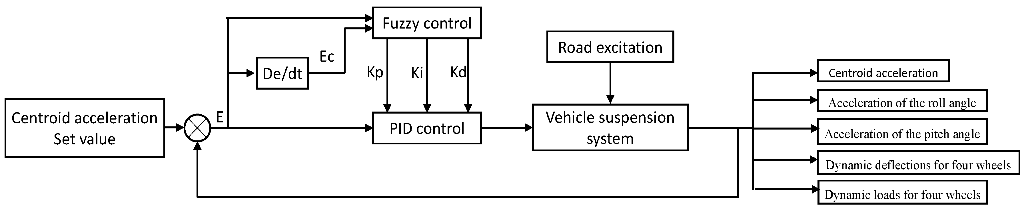
5.2. Fuzzy PID Control Algorithm

The fuzzy PID control block diagram is shown in Figure 11. The external disturbance of the vehicle suspension system is road excitation. The centroid acceleration is set to 0 mm/s², and the input of the fuzzy controller is the deviation e and the variation of the deviation ec. Based on fuzzy control rules, PID parameters are adjusted online to meet different requirements for PID parameters with different deviations e and incremental deviations ec. The simulation employs a variable-step solver with a maximum sampling step of 0.01 s, utilizing the Ode45 solver algorithm. The simulation is set to run for a duration of 5 s. The actives of the simulation are centroid acceleration, acceleration of the roll angle, acceleration of the pitch angle, dynamic deflections for four wheels, and dynamic loads for four wheels.

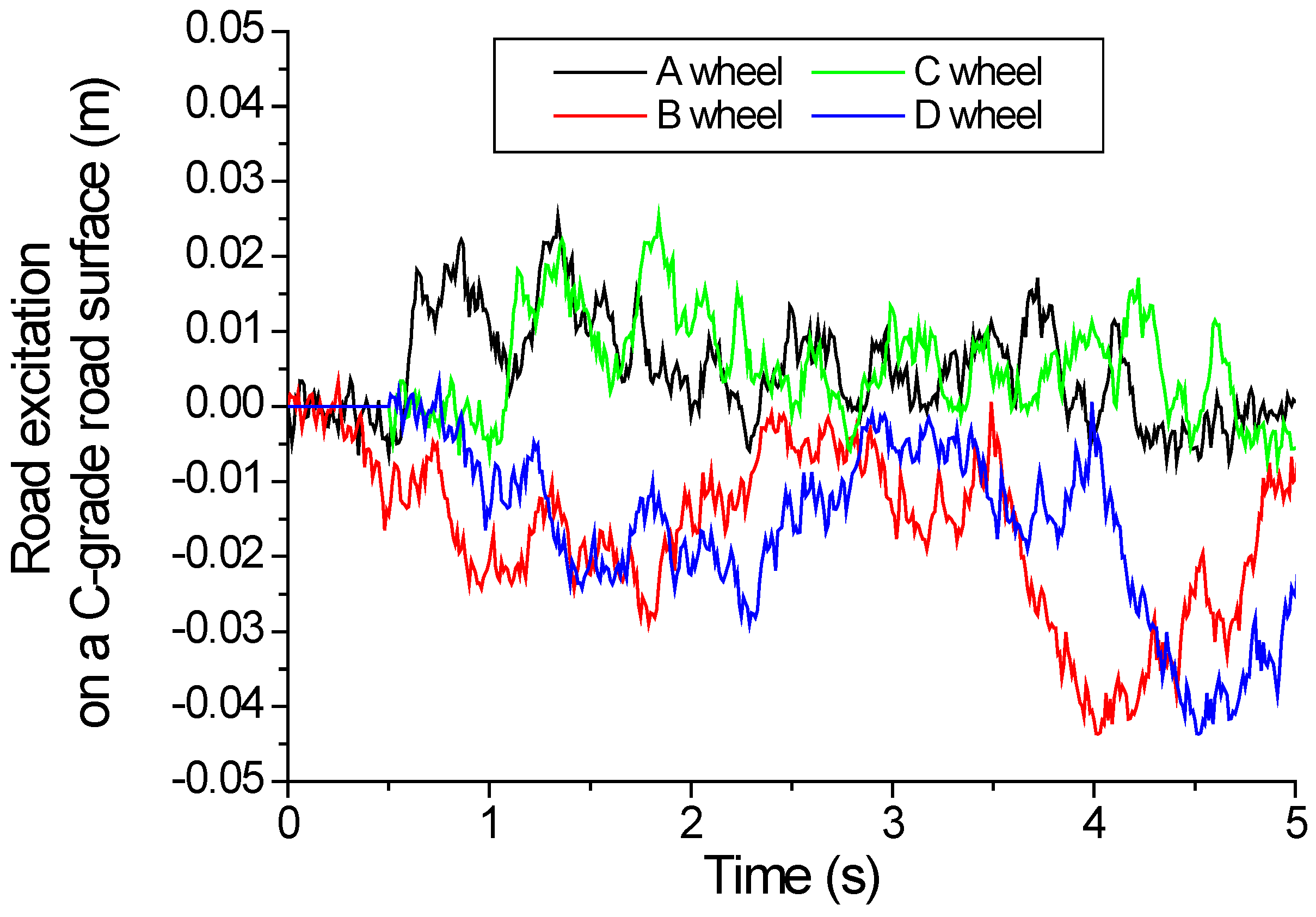
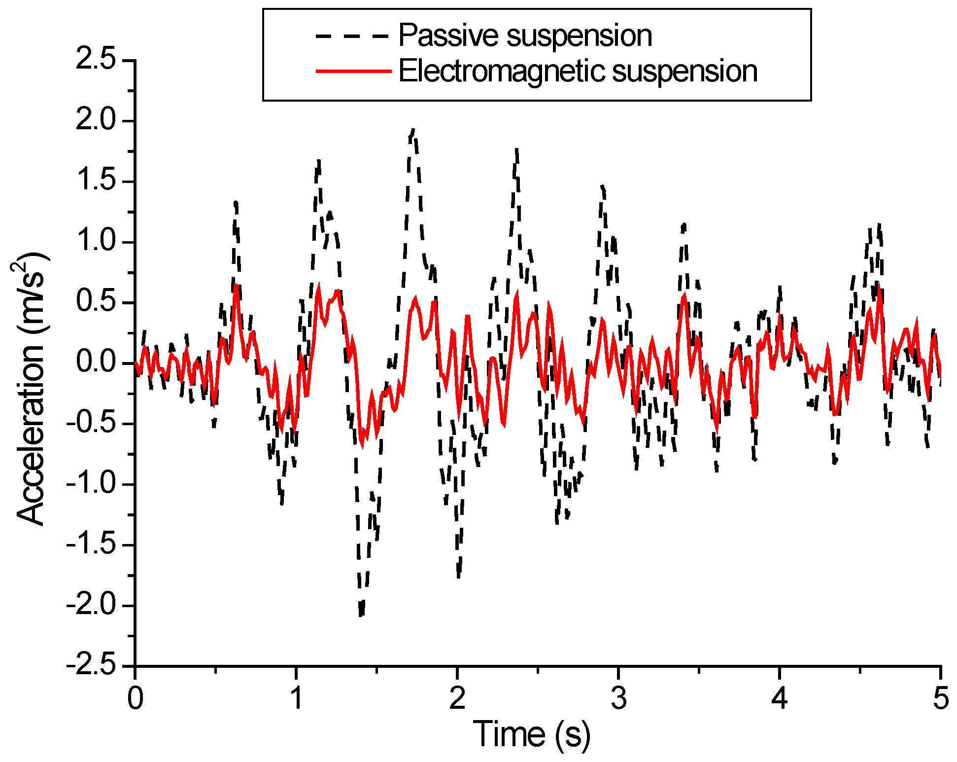
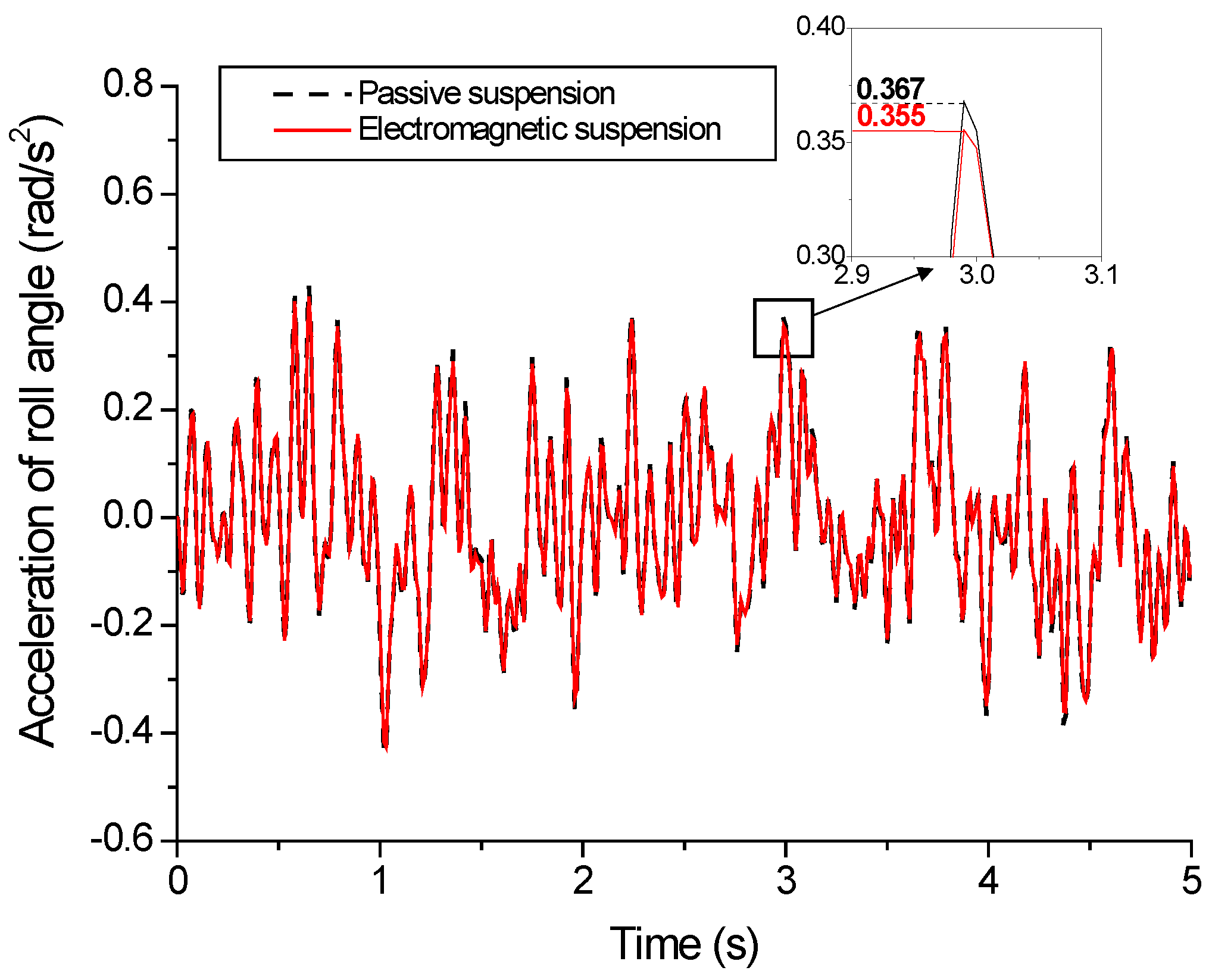
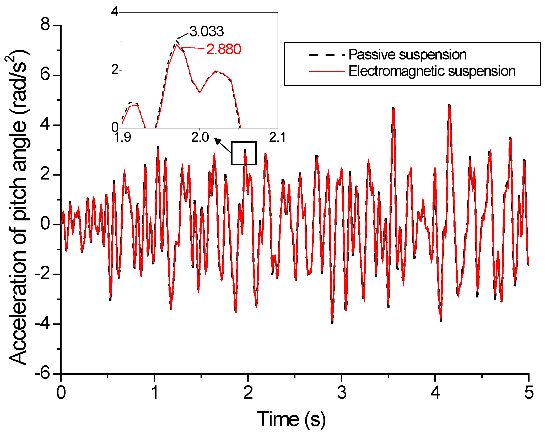
5.3. Vehicle Simulation Results Based on Fuzzy PID under C-Grade Surface

Based on Matlab/Simulink simulation software, the fuzzy PID control simulation analysis of electromagnetic suspension is carried out and compared with the passive suspension. Three evaluation indicators of vehicle ride comfort are analyzed, namely body acceleration, roll angle, and pitch angle. Take the C-grade road surface (as shown in Figure 12) as the input road surface and set the vehicle speed to 20 km/h. The fuzzy PID simulation parameters are adjusted and determined by the parameter setting method. Therefore, the fuzzy PID control law is shown in

Table 8. Control law on C-grade road surface for fuzzy PID algorithm.

U		Ec
		NB	NM	NS	Z	PS	PM	PB
E	NB	PB	PB	PM	PM	PS	Z	Z
	NM	PB	PB	PM	PS	PS	Z	NS
	NS	PM	PM	PS	PS	Z	NS	NS
	Z	PM	PM	PS	Z	NS	NM	NM
	PS	PS	PS	Z	NS	NS	NM	NM
	PM	PS	Z	NS	NM	NM	NM	NB
	PB	Z	Z	NM	NM	NM	NB	NB

. The PID control parameters are k_p = 1, k_i = 20, and k_d = 0.01.

The simulation results of centroid acceleration, acceleration of the roll angle, and acceleration of the pitch angle based on the fuzzy PID controller are shown in Figure 13, Figure 14 and Figure 15, which show the simulation comparison results of three main evaluation indicators. The trend of active suspension and passive suspension of the three curves is the same. The root mean square (RMS) values of the centroid acceleration, acceleration of the roll angle, and acceleration of the pitch angle are 59.08%, 3.06%, and 3.54% higher than those of passive suspension, respectively. The tracking response of these three curves is fast.

In the simulation results of vehicle body acceleration in Figure 13, there is a slight delay, with a delay time of 0.05 s. The acceleration of roll angle curve is shown in Figure 14. At 3 s, the peak value of the electromagnetic suspension is 0.012 rad/s² less than that of the passive suspension. The acceleration of the pitch angle curve is shown in Figure 15. At 1.96 s, the maximum value of the electromagnetic suspension is 0.153 rad/s² less than that of the passive suspension.

The simulation results of the dynamic deflections for the four wheels are shown in Figure 16. The simulation results of the suspension’s dynamic deflection for wheels A, B, C, and D are analyzed. The simulation results show that the maximum dynamic deflections of the electromagnetic active suspension are slightly lower than those of the passive suspension, and the controller has good tracking performance. The suspension dynamic deflections of wheels A, B, C, and D are 13.20%, 9.84%, 11.98%, and 16.42%, respectively, which are lower than the corresponding root mean square (RMS) value of the passive suspension.

The simulation results of the dynamic load for four wheels are shown in Figure 17. The dynamic load is closely related to the tire operation life and the impact of road damage. The simulation results show that the dynamic load of the four wheels of the electromagnetic suspension is less than the dynamic load of the passive suspension, which can reduce the impact of the tire on the road and the wear of the tire itself. The dynamic loads of the tires for the electromagnetic suspension show partial attenuation near each peak. The RMS values of the dynamic loads of wheels A, B, C, and D are 2.87%, 1.42%, 2.09%, and 5.04% lower than those of the passive suspension, respectively.

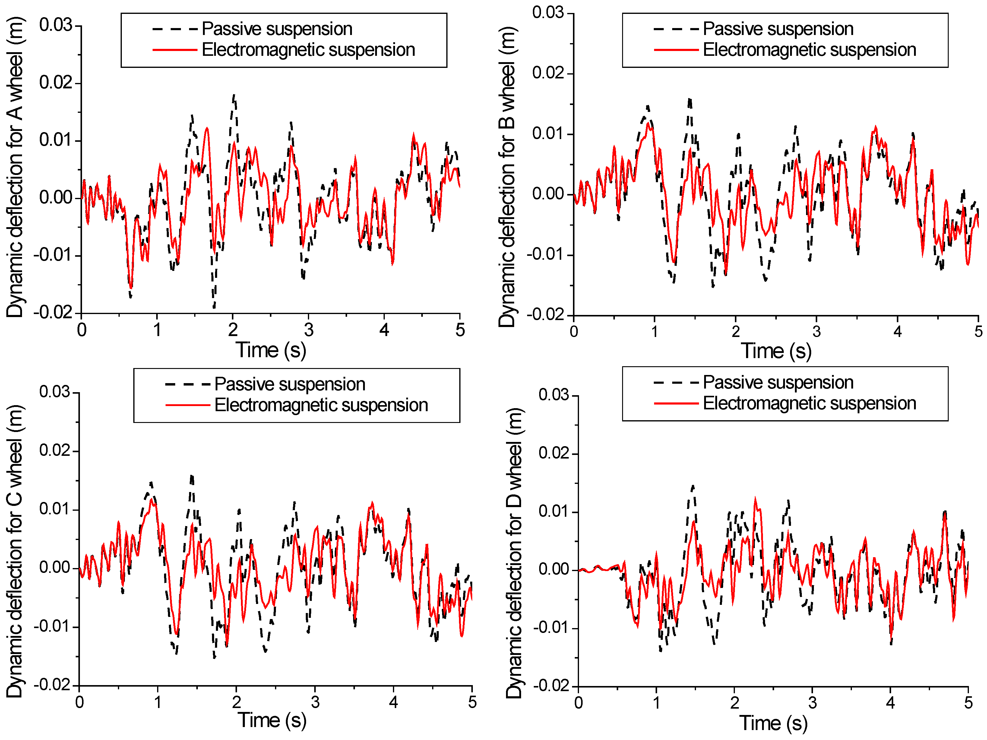
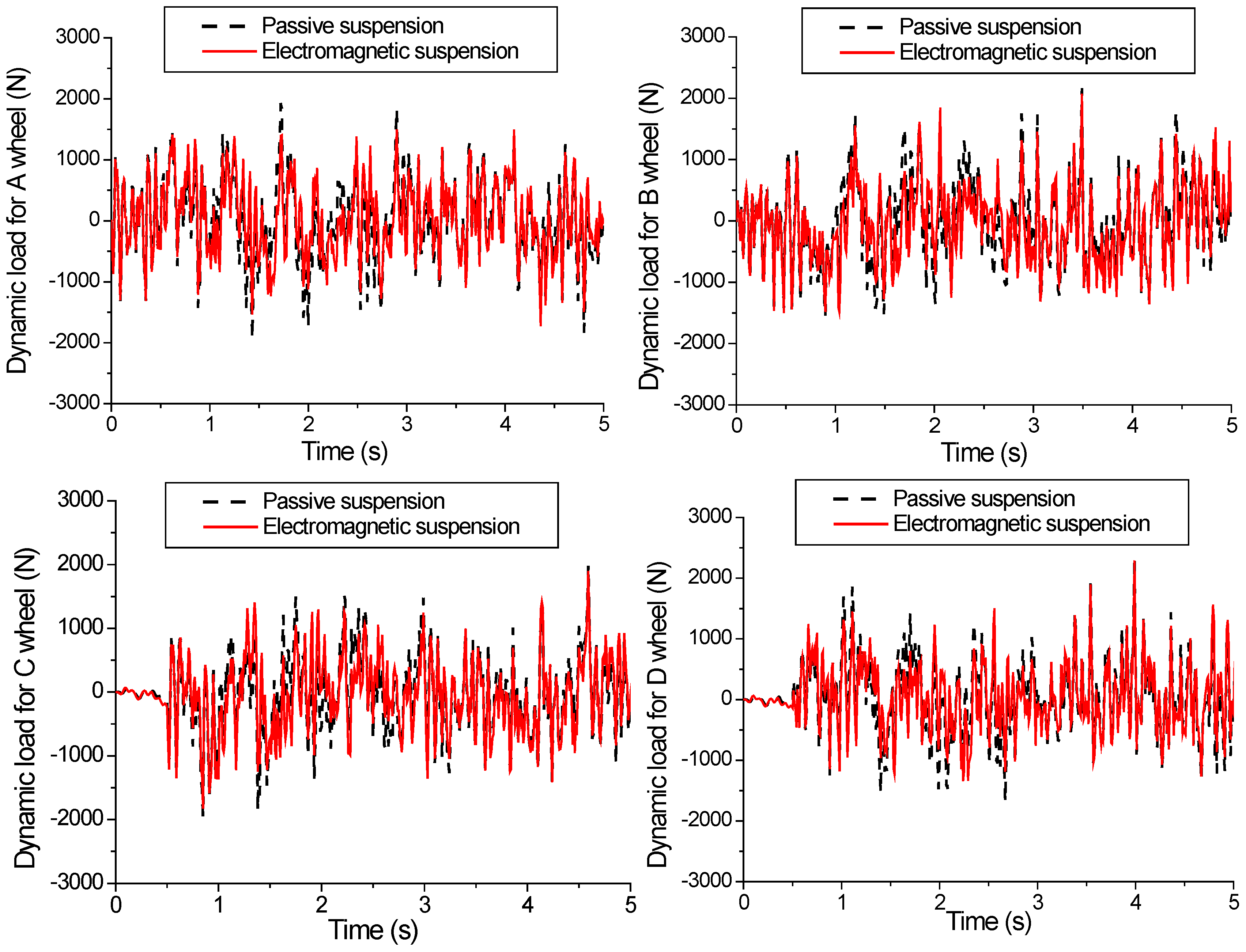
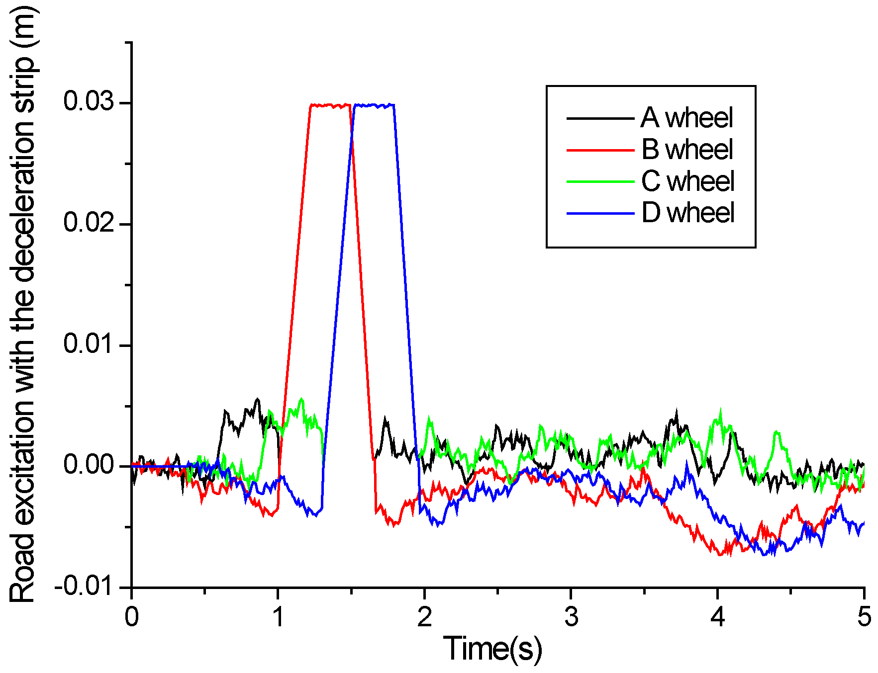
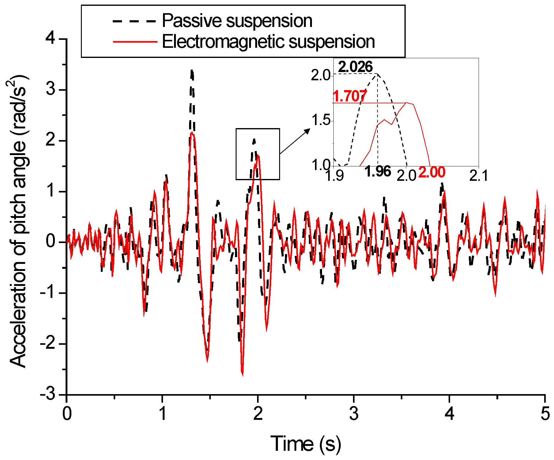
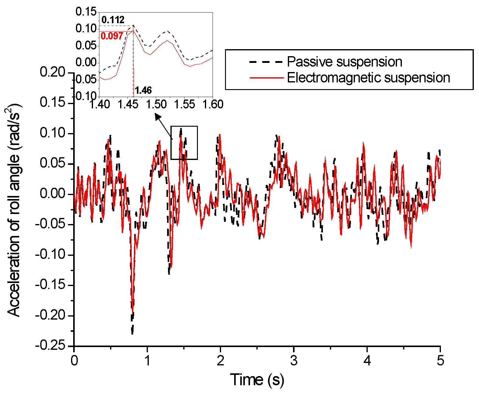
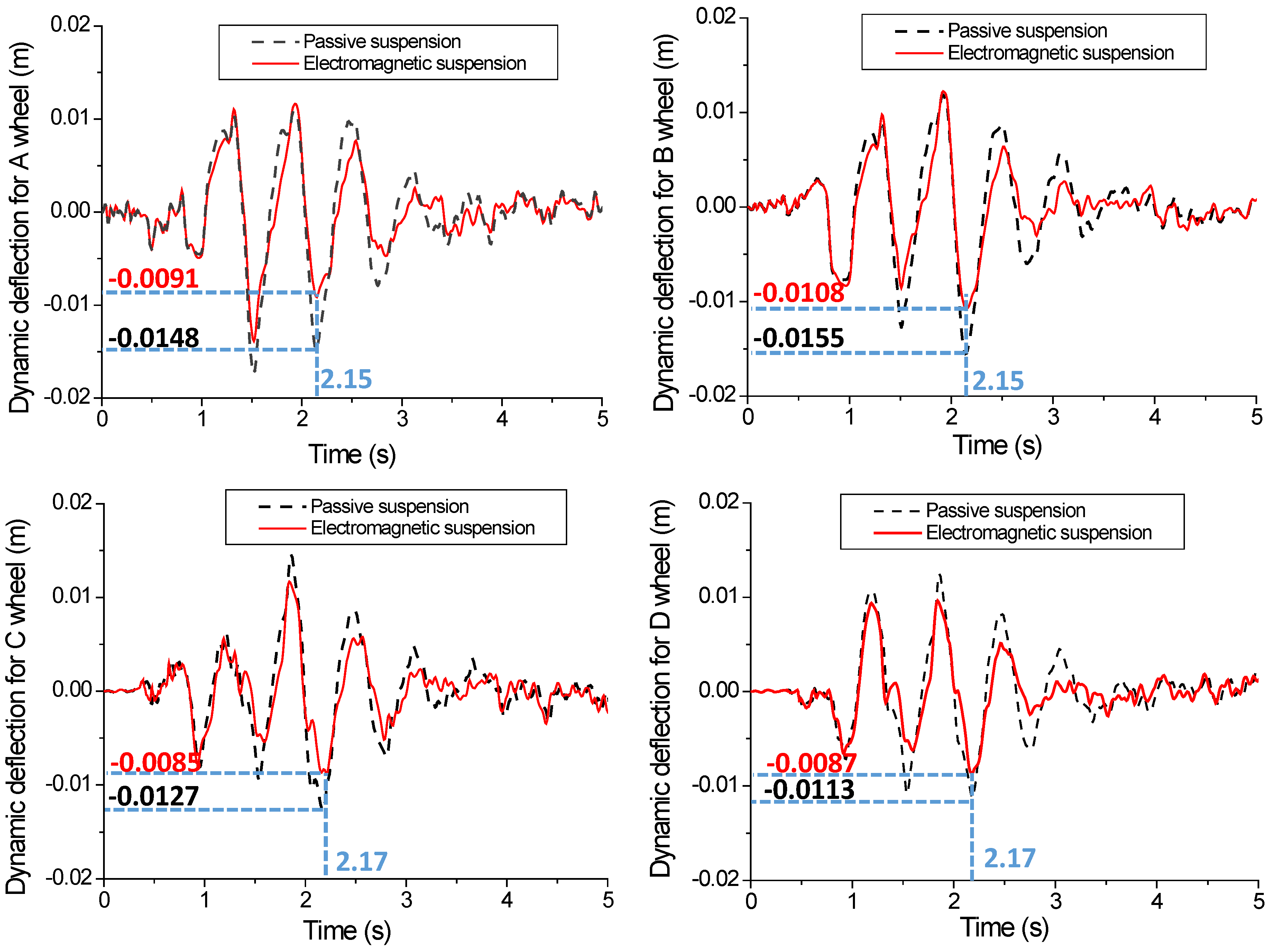
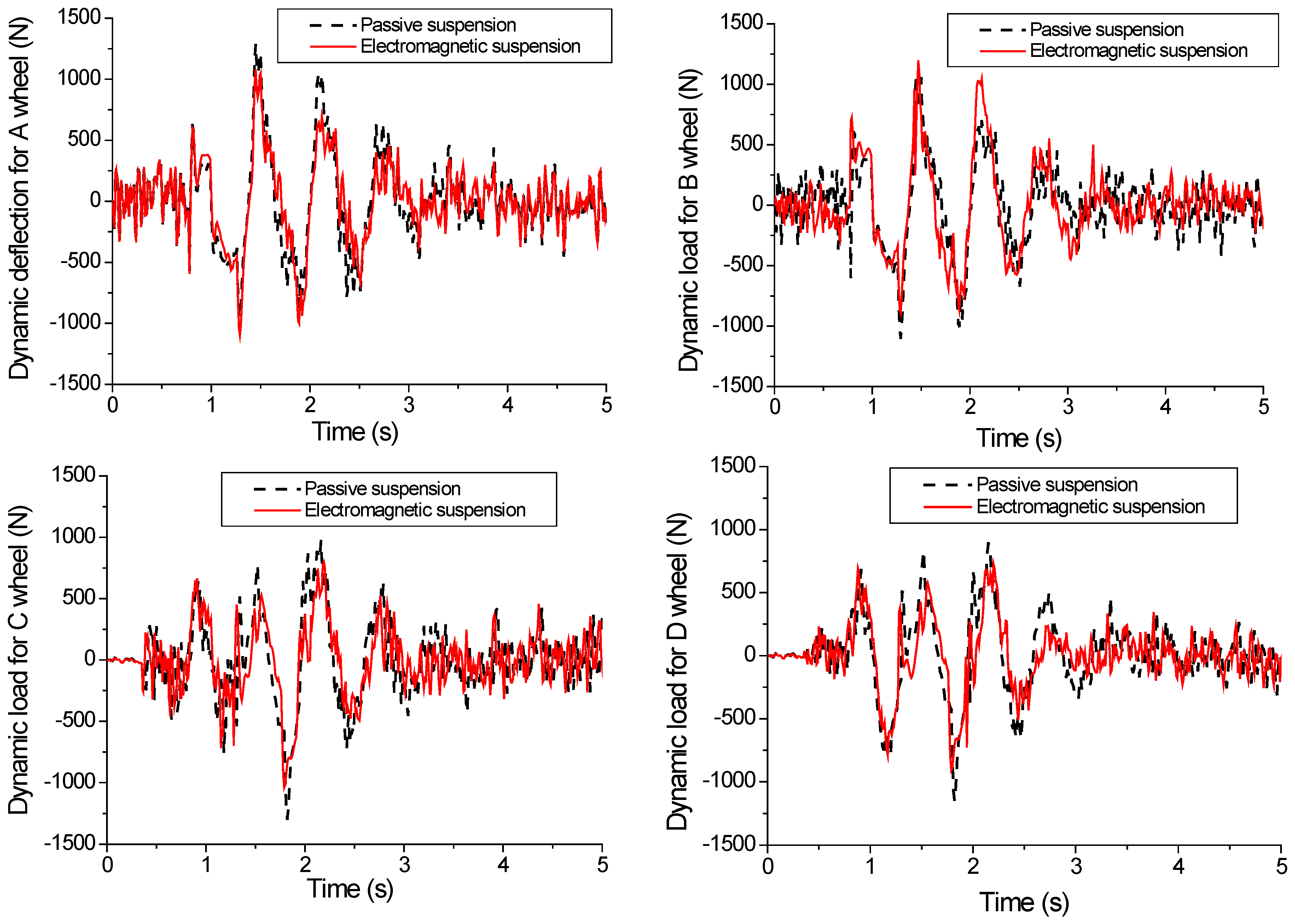
5.4. Vehicle Simulation Results Based on Fuzzy PID under a Deceleration Strip Surface

Based on the simulation on a C-level road surface in Section 5.3, a road excitation with a deceleration strip is introduced as shown in Figure 18. The deceleration strip adopts a trapezoidal shape with an upper edge of 200 mm, a lower edge of 400 mm, and a height of 30 mm. A fuzzy PID control simulation analysis was conducted on the electromagnetic suspension and compared with the passive suspension with a vehicle speed of 20 km/h. The fuzzy PID simulation parameters are adjusted and determined by setting the parameters. The fuzzy PID control law is shown in

Table 9. Control law with a deceleration strip for fuzzy PID algorithm.

U		Ec
		NB	NM	NS	Z	PS	PM	PB
E	NB	PB	PB	PM	PM	PS	Z	Z
	NM	PB	PB	PM	PS	PS	Z	NS
	NS	PM	PM	PS	PS	Z	NS	NS
	Z	PM	PM	PS	Z	NS	NM	NM
	PS	PS	PS	Z	NS	NS	NM	NM
	PM	PS	Z	NS	NS	NM	NB	NB
	PB	Z	Z	NM	NM	NM	NB	NB

. The PID control parameters are k_p = 0.8, k_i = 50, and k_d = 0.001. This simulation analysis can provide a detailed analysis of the pitch and roll characteristics to showcase the advantages of the electromagnetic suspension.

The simulation results of the centroid acceleration, acceleration of the roll angle, and acceleration of the pitch angle based on a fuzzy PID controller are shown in Figure 19, Figure 20 and Figure 21, which show the simulation comparison results of the three main evaluation indicators. The RMS values of the centroid acceleration, acceleration of the roll angle, and acceleration of the pitch angle of active suspension are 33.34%, 4.82%, and 4.10% higher than those of passive suspension, respectively.

The centroid acceleration result shows that the tracking performance of acceleration is good without any delay phenomena. At 2.13 s, the peak value of centroid acceleration using electromagnetic suspension is 0.557 m/s² smaller than when using passive suspension. In the simulation results of the acceleration of the roll angle, there is a slight delay, with a delay time of 0.04 s. The peak values of the accelerations of the roll angle and the pitch angle decreased by 0.319 rad/s² and 0.015 rad/s², respectively.

The dynamic deflections of the four wheels of the vehicle are shown in Figure 22. The RMS values of the dynamic deflection of wheels A, B, C, and D decreased by 21.26%, 21.40%, 25.01%, and 24.24%, respectively. When the rear wheels pass through the reducer, the shock absorbers generate a downward dynamic deflection. After fuzzy PID control, the dynamic deflections of the four dampers decrease by 0.0057 m, 0.0047 m, 0.0042 m, and 0.0026 m, respectively. The fluctuation of the rear wheel is delayed by 0.02 s relative to the fluctuation of the front wheel. The dynamic deflections of the four wheels of the passive suspension are −0.0148 m, −0.0155 m, −0.0127 m, and −0.0113 m, and it can be seen that the difference between the maximum and minimum is 0.0042 m. The dynamic deflections of wheels A, B, C, and D of the electromagnetic suspension are −0.0091 m, −0.0108 m, −0.0085 m, and −0.0087 m, and it can be seen that the difference between the maximum and minimum is 0.0023 m. These results indicate that electromagnetic suspension can be effectively controlled on a deceleration strip or when braking, which makes up for the poor stability of the MacPherson suspension.

The simulation results of the dynamic load for the four wheels are shown in Figure 23. The RMS values of the dynamic loads of wheels A, B, C, and D are 11.43%, 11.91%, 14.91%, and 15.03% lower than those of the passive suspension, respectively. When passing through the deceleration strip, the dynamic loads of the front wheel tires are larger than those of the rear wheel tires. The results show that when the vehicle passes through the deceleration strip, the dynamic load of the tires can be reduced and the excessive friction of the tires can be effectively prevented via the fuzzy PID control algorithm.

6. Conclusions

This paper proposes an electromagnetic suspension that can ensure the safety of a vehicle and improve the ride comfort and stability of the MacPherson suspension. This suspension does not change the safety of the MacPherson suspension with embedding an electromagnetic actuator. Once the electromagnetic actuator fails, the safety of the electromagnetic suspension can be guaranteed.

This paper mainly studies its magnetic characteristics and fuzzy PID control. First, an electromagnetic suspension is proposed, and its theoretical magnetic field model is established and analyzed. Second, on the basis of the electromagnetic suspension system, a FEM model is established, and the magnetic field, magnetic flux density, and magnetic force are simulated and analyzed. Finally, on the basis of the fuzzy PID control algorithm, a vehicle simulation analysis of the electromagnetic suspension is carried out. The results show that the magnetic field trends of the theoretical results and the finite element results are consistent via a comparison. The direction and the trend of the magnetic flux density in the FEM simulation show that the magnetic fluxes are parallel to each other in the air gap of the magnet assembly. Comparing the theoretical results, finite element results, and experimental results in [44], the electromagnetic suspension proposed in this paper owns a larger magnetic flux density in the air gap. At the same time, it can also prove the correctness of the trend of the theoretical results and the feasibility of the proposed electromagnetic actuator. Based on the fuzzy PID control algorithm, the vehicle dynamics of the electromagnetic suspension are simulated. The simulation results show that compared to a passive suspension system, RMS values of the acceleration, the acceleration of roll angle, and the acceleration of pitch angle for the vehicle body are reduced by 59.08%, 3.06%, and 3.54%, respectively, and the dynamic deflection of the four suspension systems and the dynamic load of the four wheels are reduced. Therefore, this control algorithm is suitable for an electromagnetic suspension system.

In the future, we will build an experimental prototype of this electromagnetic actuator for magnetic field and current experiments. At the same time, research is being conducted on the stability and smoothness control of electromagnetic suspension with extreme road surfaces.

References

1. Tseng, H.E.; Hrovat, D. State of the art survey: Active and semi-active suspension control. Veh. Syst. Dyn. 2015, 53, 1034–1062. [Google Scholar] [CrossRef]
2. Cao, D.; Song, X.; Ahmadian, M. Editors’ perspectives: Road vehicle suspension design, dynamics, and control. Veh. Syst. Dyn. 2011, 49, 3–28. [Google Scholar] [CrossRef]
3. Kim, K.H.; Woo, D.K. Linear tubular permanent magnet motor for an electromagnetic active suspension system. IET Electr. Power Appl. 2021, 15, 1648–1665. [Google Scholar] [CrossRef]
4. Zhou, H.; Zhen, L.; Zhao, W.; Liu, G.; Xu, L. Design and analysis of low-cost tubular fault-tolerant interior permanent-magnet motor. IEEE Trans. Magn. 2016, 52, 8104804. [Google Scholar] [CrossRef]
5. Basaran, S.; Basaran, M. Vibration control of truck cabins with the adaptive vectorial backstepping design of electromagnetic active suspension system. IEEE Access 2020, 8, 173056–173067. [Google Scholar] [CrossRef]
6. Harikrishnan, P.M.; Varun, P.G. Vehicle vibration signal processing for road surface monitoring. IEEE Sens. J. 2017, 17, 5192–5197. [Google Scholar] [CrossRef]
7. Majdoub, K.E.; Giri, F.; Chaoui, F.Z. Adaptive backstepping control design for semi-active suspension of half-vehicle with magnetorheological damper. IEEE/CAA J. Autom. Sin. 2022, 8, 582–596. [Google Scholar] [CrossRef]
8. Envelope, K.; Envelope, K.H. Vibration control of semi-active suspension by the neural network that learned the optimal preview control of MLD model. IFAC-Pap. 2022, 55, 515–520. [Google Scholar]
9. Basargan, H.; Mihály, A.; Gáspár, P.; Sename, O. An LPV-based online reconfigurable adaptive semi-active suspension control with MR damper. Energies 2022, 15, 3648. [Google Scholar] [CrossRef]
10. Liu, W.; Wang, R.; Ding, R.; Meng, X.; Yang, L. On-line estimation of road profile in semi-active suspension based on unsprung mass acceleration. Mech. Syst. Signal Process. 2020, 135, 106370. [Google Scholar] [CrossRef]
11. Beno, J.H.; Weeks, D.A.; Bresie, D.A.; Guenin, A.M.; Wisecup, J.S.; Bylsma, W. Experimental comparison of losses for conventional passive and energy efficient active suspension systems. SAE Technical Paper Series. In Proceedings of the SAE International SAE 2002 World Congress & Exhibition, Detroit, MI, USA, 4 May 2002. SAE Technology Paper, 2002-01-0282. [Google Scholar]
12. Weeks, D.A.; Beno, J.H.; Guenin, A.M.; Bresie, D.A. Electro mechanical active suspension demonstration for off-road vehicles. In Direct Injection SI Engine Technology, Proceedings of the SAE 2000 World Congress, Detroit, MI, USA, 6 March 2000; SAE International: Warrendale, PA, USA, 2000; SAE Technology Paper, 2000-01-0102. [Google Scholar]
13. Bylsma, W.; Guenin, A.M.; Beno, J.H.; Weeks, D.A.; Bresie, D.A.; Raymond, M.E. Electromechanical suspension performance testing. SAE Technical Paper Series. In Proceedings of the 2001 SAE International SAE 2001 World Congress, Detroit, MI, USA, 5–8 March 2001. SAE Technology Paper, 2001-01-0492. [Google Scholar]
14. Hayes, R.J.; Beno, J.H.; Weeks, D.A.; Guenin, A.M.; Mock, J.R.; Worthington, M.S.; Triche, E.J.; Chojecki, D.; Lippert, D. Design and testing of an active suspension system for a 2-1/2 ton military truck. SAE Technology Paper. In Proceedings of the SAE International SAE 2005 World Congress & Exhibition, Detroit, MI, USA, 11 April 2005. SAE Technology Paper, 2005-01-1715. [Google Scholar]
15. Yu, F.; Cao, M.; Zheng, X.C. Research on the feasibility of vehicle active suspension with energy regeneration. Vib. Shock. 2005, 24, 27–30. [Google Scholar]
16. Yu, F.; Fang, T.; Pattipati, K.R. A novel congruent organizational design methodology using group technology and a nested genetic algorithm. IEEE Trans. Syst. Man Cybern. Part A Syst. Hum. 2005, 36, 5–18. [Google Scholar]
17. Zhang, Y.C.; Yu, F.; Gu, Y.H. Isolation and energy-regenerative performance experimental verification of automotive electrical suspension. J. Shanghai Jiaotong Univ. 2008, 42, 874–877. [Google Scholar]
18. Huang, K.; Yu, F.; Zhang, Y.C. Model predictive controller design for electromagnetic active suspension. J. Shanghai Jiaotong Univ. 2010, 44, 1619–1624. [Google Scholar]
19. Huang, S.J.; Chen, H.Y. Adaptive sliding controller with self-tuning fuzzy compensation for vehicle suspension control. Mechatronics 2006, 16, 607–622. [Google Scholar] [CrossRef]
20. Kawamoto, Y.; Suda, Y.; Inoue, H.; Kondo, T. Modeling of electromagnetic damper for automobile suspension. J. Syst. Des. Dyn. 2007, 1, 524–535. [Google Scholar] [CrossRef]
21. Hayashi, R.; Suda, Y.; Nakano, K. Anti-rolling suspension for an automobile by coupled electromagnetic devices. J. Mech. Syst. Transp. Logist. 2008, 1, 43–55. [Google Scholar] [CrossRef]
22. Kawamoto, Y.; Suda, Y.; Inoue, H.; Kondo, T. Electro-mechanical suspension system considering energy consumption and vehicle manoeuvre. Veh. Syst. Dyn. 2008, 46, 1053–1063. [Google Scholar] [CrossRef]
23. Asadi, E.; Ribeiro, R.; Khamesee, M.B.; Khajepour, A. Analysis, prototyping and experimental characterization of an adaptive hybrid-electromagnetic damper for automotive suspension systems. IEEE Trans. Veh. Technol. 2017, 66, 3703–3713. [Google Scholar] [CrossRef]
24. Liu, Y.; Xu, L.; Zuo, L. Design, modeling, lab, and field tests of a mechanical-motion-rectifier-based energy harvester using a ball-screw mechanism. IEEE/ASME Trans. Mechatron. 2017, 22, 1933–1943. [Google Scholar] [CrossRef]
25. Eckert, P.R.; Flores Filho, A.F.; Perondi, E.A.; Dorrell, D.G. Dual quasi-halbach linear tubular actuator with coreless moving-coil for semiactive and active suspension. IEEE Trans. Ind. Electron. 2018, 65, 9873–9883. [Google Scholar] [CrossRef]
26. Eckert, P.R.; Flores Filho, A.F.; Perondi, E.; Ferri, J.; Goltz, E. Design Methodology of a Dual-Halbach Array Linear Actuator with Thermal-Electromagnetic Coupling. Sensors 2016, 16, 360. [Google Scholar] [CrossRef] [PubMed]
27. Beltran-Carbajal, F.; Valderrabano-Gonzalez, A.; Favela-Contreras, A. An active vehicle suspension control approach with electromagnetic and hydraulic actuators. Actuators 2019, 8, 35. [Google Scholar] [CrossRef]
28. Ning, D.; Du, H.; Sun, S.; Zheng, M.; Li, W.; Zhang, N.; Jia, Z. An electromagnetic variable stiffness device for semiactive seat suspension vibration control. IEEE Trans. Ind. Electron. 2020, 67, 6773–6784. [Google Scholar] [CrossRef]
29. Wang, J.J.; Cai, Y.F.; Chen, L.; Shi, D.; Wang, S.; Zhu, Z. Research on compound coordinated control for a power-split hybrid electric vehicle based on compensation of non-ideal communication network. IEEE Trans. Veh. Technol. 2020, 69, 14818–14833. [Google Scholar] [CrossRef]
30. Wang, J.J.; Cai, Y.F.; Chen, L.; Shi, D.; Wang, R.; Zhu, Z. Review on multi-power sources dynamic coordinated control of hybrid electric vehicle during driving mode transition process. Int. J. Energy Res. 2020, 44, 6128–6148. [Google Scholar] [CrossRef]
31. Wei, W.; Li, Q.; Xu, F.; Zhang, X.; Jin, J.; Jin, J.; Sun, F. Research on an electromagnetic actuator for vibration suppression and energy regeneration. Actuators 2020, 9, 42. [Google Scholar] [CrossRef]
32. Wei, W.; Sun, F.; Jin, J.Q.; Zhao, Z.Y.; Miao, L.G.; Li, Q.; Zhang, X.Y. Proposal of energy-recycle type active suspension using magnetic force. Int. J. Appl. Electromagn. Mech. 2019, 59, 577–585. [Google Scholar] [CrossRef]
33. Ye, X.M.; Long, H.Y.; Pei, W.C.; Li, Y.G.; Zhang, S.; Chu, J. Fuzzy control of automotive magnetorheological semi-active suspension. J. North China Univ. Sci. Technol. 2018, 40, 79–87. [Google Scholar]
34. Bashir, A.O.; Rui, X.; Zhang, J. Ride comfort improvement of a semi-active vehicle suspension based on hybrid fuzzy and fuzzy-PID controller. Stud. Inform. Control. 2019, 28, 421–430. [Google Scholar] [CrossRef]
35. El-Taweel, H.; Elhafiz, M.; Metered, H. Vibration Control of Active Vehicle Suspension System Using Optimized Fuzzy-PID. SAE Technical Paper Series. In Proceedings of the WCX World Congress Experience, Detroit, MI, USA, 3 April 2018. SAE International by Univ of California Berkeley, 2018-01-1402. [Google Scholar]
36. Wang, X.; Yang, B.T.; Zhu, Y. Adaptive model-based feedforward to compensate Lorentz force variation of voice coil motor for the fine stage of lithographic equipment. Optik 2019, 135, 27–35. [Google Scholar] [CrossRef]
37. Lian, J.Q.; Xie, S.Y.; Wang, J. Analysis of cogging torque of PM motor with radial magnetic field and parallel magnetic field. Appl. Mech. Mater. 2011, 105–107, 2289–2294. [Google Scholar] [CrossRef]
38. Jing, L.B.; Zhang, Y.S.; Li, C.; Zhang, K. Magnetic field computa-tion and optimization design for a concentric magnetic gear with hal-bach permanent-magnet arrays. Proc. CSEE 2013, 33, 163–169. [Google Scholar]
39. Wang, X.; Yang, B.T.; Zhu, Y. Modeling and analysis of a novel rectan-gular voice coil motor for the 6-DOF fine stage of lithographic equip-ment. Optik 2016, 127, 2246–2250. [Google Scholar] [CrossRef]
40. Liu, Y.; Zhang, M.; Zhu, Y. Optimization of voice coil motor to enhance dynamic response based on an improved magnetic equivalent circuit model. IEEE Trans. Magn. 2011, 47, 2247–2251. [Google Scholar] [CrossRef]
41. Babic, S.I.; Akyel, C. Improvement in the Analytical Calculation of the Magnetic Field Produced by Permanent Magnet Rings. Prog. Electromagn. Res. C 2016, 5, 71–82. [Google Scholar]
42. Xia, Z.P.; Zhu, Z.Q.; Howe, D. Senior member. analytical magnetic Field analysis of halbach Magnetized permanent-magnet machines. IEEE Trans. Magn. 2004, 40, 1864–1872. [Google Scholar] [CrossRef]
43. Chen, Y.; Zhang, K.L. Analytic calculation of the magnetic field created by Halbach permanent magnets array. J. Magn. Mater. Devices 2014, 45, 1–4. [Google Scholar]
44. Wei, W.; Li, Q.; Sun, F.; Zhang, X.Y. Vibration control and energy regeneration of active suspension based on electromagnetic actuator—Development of electromagnetic actuator. In Proceedings of the International Conference on Precision Engineering (ICPE), Hakodate, Japan, 5–7 September 2018. C03-1. [Google Scholar]
Figure 1. Structure of the electromagnetic suspension system. (a) 1/4 MacPherson-type independent suspension. (b) Electromagnetic shock absorber.
Actuators 12 00203 g001aActuators 12 00203 g001b
Figure 2. Structure of the magnet assembly.
Actuators 12 00203 g002
Figure 3. Dimensional drawing. (a) Sectional view in the radial direction. (b) Sectional view in the axial direction.
Actuators 12 00203 g003
Figure 4. Schematic diagram of the magnetic field of a single PM ring.
Actuators 12 00203 g004
Figure 5. Theoretical results of magnetic flux density.
Actuators 12 00203 g005
Figure 6. FEM analysis of magnetic field for half of the actuator. (a) The magnetic flux density. (b) The direction of magnetic flux. (c) The trend of magnetic flux.
Actuators 12 00203 g006aActuators 12 00203 g006b
Figure 7. Simulation results of magnetic flux density.
Actuators 12 00203 g007
Figure 8. Three results of magnetic flux density.
Actuators 12 00203 g008
Figure 9. Simulation results of magnetic force characteristics. (a) The current–magnetic force curve. (b) The displacement–magnetic force curve.
Actuators 12 00203 g009
Figure 10. Seven-DOF dynamics model based on fuzzy PID control.
Actuators 12 00203 g010
Figure 11. Fuzzy PID control block diagram.
Actuators 12 00203 g011
Figure 12. Road excitation on a C-grade road surface for four wheels.
Actuators 12 00203 g012
Figure 13. Centroid acceleration on a C-grade road surface.
Actuators 12 00203 g013
Figure 14. Acceleration of the roll angle on a C-grade road surface.
Actuators 12 00203 g014
Figure 15. Acceleration of the pitch angle on a C-grade road surface.
Actuators 12 00203 g015
Figure 16. Dynamic deflections on a C-grade road surface for four wheels.
Actuators 12 00203 g016
Figure 17. Dynamic loads on a C-grade road surface for four wheels.
Actuators 12 00203 g017
Figure 18. Road excitation with the C deceleration strip for four wheels.
Actuators 12 00203 g018
Figure 19. Centroid acceleration on a deceleration strip.
Actuators 12 00203 g019
Figure 20. Acceleration of the roll angle on a deceleration strip.
Actuators 12 00203 g020
Figure 21. Acceleration of the pitch angle on a deceleration strip.
Actuators 12 00203 g021
Figure 22. Dynamic deflections on a deceleration strip for four wheels.
Actuators 12 00203 g022
Figure 23. Dynamic loads on a deceleration strip for four wheels.
Actuators 12 00203 g023