Abstract
This paper presents a comparative study on the effects of the input configurations of linear quadratic (LQ) controllers on path tracking performance under low friction conditions. For the last decade, the path tracking controller has adopted several control inputs, input configurations, and actuators. However, these have not been compared with one another on a single frame in terms of common measures. For this reason, this paper compares input configurations of LQ controllers and available actuators in terms of common measures. For this purpose, the control inputs of the LQ controller were composed of front and rear steering and control yaw moment. By combining these control inputs, five input configurations of the LQ controller were set. If the control yaw moment is selected as a control input, then an actuator is needed to generate a control allocation, which should be adopted to convert the control yaw moment into longitudinal and lateral tire forces of actuators. As an actuator for control yaw moment generation, front/rear and 4-wheel steering, 4-wheel independent steering, braking, and driving were adopted. By applying the weighted least square based method, control allocation was formulated as a quadratic programming problem, which can be algebraically solved. For comparison on path tracking performance, new measures were adopted. To check the path tracking performance of each input configuration, a simulation was conducted on vehicle simulation software. From the simulation results, it was shown that front or 4-wheel steering itself is enough for path tracking on low friction roads and that the control yaw moment or an additional actuator is not recommended as a control input for path tracking on low friction roads.
1. Introduction
For the last decade, a lot of papers have been published on autonomous driving, which is regarded as an emerging solution for future transportation in the automotive industry and research community [1,2,3]. According to the literature on autonomous driving, it is known that a generic modular system pipeline for autonomous driving consists of object detection, tracking, localization, assessment, behavior prediction, planning, and control [2]. Among these topics of autonomous driving, the last step is path tracking control (PTC), which has also been intensively studied [4,5]. As a result of intensive study on PTC, a great deal of papers have also been published for the last decade in the area of PTC [4,5,6,7,8,9,10]. This paper focuses on PTC.
Compared to a lot of papers focusing on PTC on high friction roads, a small number of papers focusing on PTC under low friction conditions have been published since 2015 [11,12,13,14,15,16,17,18,19,20,21,22,23,24,25,26,27,28]. Most of these papers adopted linear quadratic regulator (LQR) and model predictive control (MPC) as controller design methodologies. However, the input configurations and available actuators were different from one another. For this reason, it is necessary to compare those controllers on a single framework in terms of some measures for path tracking performance. For this purpose, this paper compares the input configurations and available actuators of LQR-based path tracking controllers.
From the literature survey, the common features of the papers focusing on LQ path tracking controllers can be summarized into three categories: input configurations of LQ controllers, actuator combinations corresponding to input configuration, and driving conditions [11,12,13,14,15,16,17,18,19,20,21,22,23,24,25,26,27,28]. These features are investigated in this paper.
In view of input configuration, several control inputs such as front and rear steering angles and control yaw moment have been combined in LQ path tracking controllers such as a linear quadratic regulator (LQR), a model predictive control (MPC), and an H∞ control. Among these, MPC is the most widely adopted controller for PTC [11,13,14,17,19,20,21,22,23,24,25,26,27,28]. The advantage of these controllers is that it is easy to combine several types of control inputs. For example, the most commonly selected input configuration in LQR and MPC is the combination of front wheel steering (FWS), δf, and longitudinal forces, ΔFx, [17,19,20,23,24,26]. The next is the combination of FWS and control yaw moment, ΔMz, [11,12,15,25,27]. If ΔMz is adopted in a particular input configuration, then a control allocation method or yaw moment distribution procedure is needed to convert it into longitudinal and lateral tire forces. In previous work, LQR and MPC with three input configurations, δf, [δf δr]T, and [δf ΔMz]T, were designed and compared under various speeds and friction conditions [11]. In another study, several path tracking controllers with FWS and 4WS were designed and compared with one another under high friction conditions [28,29]. Following the idea of these papers, the aim of this paper was to check the path tracking performance of several input configurations available in LQR.
In view of the actuator combination for path tracking, front wheel steering (FWS), rear wheel steering (RWS), 4-wheel steering (4WS), 4-wheel independent steering (4WIS), 4-wheel independent braking (4WIB), and 4-wheel independent driving (4WID) have been selected to date [30]. Among these, rear wheel independent steering (RWIS) has not been used as an actuator for path tracking. In this paper, 4WS stands for the combination of FWS and RWS. To date, most path tracking controllers used for autonomous driving have been designed for a vehicle with front-wheel steering (FWS), which resulted in conventional Ackerman steering being adopted for PTC [7,8]. On the other hand, the other actuators, except for FWS, have been widely adopted as actuators in the area of vehicle stability control (VSC) [30,31,32]. In this paper, the term VSC means the yaw rate tracking and lateral stability control. For the last decade, thanks to the development of in-wheel motor (IWM) systems, independent steering, braking, and driving systems such as 4WIS, 4WIB, and 4WID have become available for VSC [33,34,35]. These actuators have also been used for PTC [12,13,14,15,16,17,18,19,20,21,22,23,24,25,26,27,28,36]. Generally, FWS, RWS, and 4WS can be easily included in the input configuration of LQR as a control input. On the contrary, 4WIS, 4WIB, and 4WID cannot be included in the input configuration of LQR because the input matrix of the state-space equation cannot be derived with these actuators. To utilize these actuators for path tracking, ΔFx or ΔMz should be included in the input configuration. After calculating these control inputs, these should be converted into longitudinal and later tire force by a control allocation method. This paper checks the effects of these actuators on path tracking performance.
In view of driving condition, some path tracking controllers have been simulated on the low tire-road friction coefficient, μ [12,13,14,15,16,17,18,19,20,21,22,23,24,25,26,27,28]. In the literature, μ was set between 0.3 and 0.4. From the viewpoint of VSC, a vehicle driving on low μ roads can easily lose its lateral stability in spite of maintaining yaw rate tracking performance [37,38]. This is caused by the fact that the lateral force of low μ roads is much smaller than that on high μ ones. Generally, the lateral stability of a vehicle is measured with the side-slip angle, β [38]. For this reason, β should be kept small as not to diverge for lateral stability. The most common method for lateral stability is to add β into the quadratic objective function of LQR and MPC [12,15,17,39,40]. Another method is to use some schemes coordinating path tracking and lateral stability [17,19]. In these papers, switching criteria based on a phase plane drawn by the side-slip angle and its angular velocity were proposed. However, in LQR-based path tracking controllers, the lateral offset error rate is equivalent to the lateral velocity or side-slip angle of a vehicle. For this reason, lateral stability can be kept on low μ roads by setting higher weights on the lateral offset error rate in the LQ objective function. If this weight is set too high, then the heading error is not reduced by the controller, which results in poor path tracking performance. This tendency becomes worse if 4WS is adopted as an actuator. For this reason, exhaustive and time-consuming tuning on weights is needed for lateral stability in LQR-based path tracking controllers. In this paper, the effects of several input configurations and actuator combinations on path tracking performance are checked under low μ conditions.
The contents mentioned above are summarized in Table 1. In Table 1, the symbol FF stands for feedforward control. From Table 1, the input configurations of LQR-based path tracking controllers can be classified seven ways from IC#1 to IC#7, as given in Table 2. In Table 2, the symbol IC is the abbreviation of the input configuration. As shown in Table 2, there are four control inputs, i.e., the front and rear steering angles, δf and δr, the control yaw moment, ΔMz, and the longitudinal control tire force, ΔFx. Among these, ΔFx can be converted into ΔMz by using force-moment equilibrium with geometric dimensions such as wheelbase and tread [17,19,20]. For this reason, IC#6 and IC#7 are neglected hereafter. As a result, three control inputs, δf, δr and ΔMz, constitute five input configurations from IC#1 to IC#5.

Table 1.
Summary of the LQ-based path tracking controllers on low friction roads.
Table 2.
Input configurations, control inputs, and available actuators.
The third column of Table 2 represents the available actuators for each input configuration. For IC#1 and IC#2, FWS and 4WS are available, respectively. For this reason, the other actuators should not be set to IC#1 and IC#2 because they will break the optimality of the FWS and 4WS of IC#1 and IC#2. For IC#3, RWS, RWIS, 4WIB, and 4WID are available because these actuators can generate ΔMz. However, 4WS or 4WIS cannot be used for IC#3 because they will break the optimality of FWS in IC#3. If active front steering (AFS) is assumed to be available, then 4WS can be used for IC#3. However, it is assumed that AFS is not available in this paper. For IC#4, only 4WIB and 4WID are available because 4WS is already set in IC#3. In fact, 4WIS cannot be used for the input configuration with FWS and 4WS, i.e., IC#1, IC#2, IC#3, and IC#4, because it will break the optimality of the control inputs of these input configurations. On the other hand, all the actuators, i.e., FWS, 4WS, 4WIS, 4WIB, and 4WID, are available for IC#5 because there are no actuators set to IC#5. The relationship between the input configurations and actuators is captured in a control allocation method.
The aim of this paper was to check the path tracking performance of five input configurations of LQR with various actuator combinations on low μ roads. Figure 1 shows the schematic diagram of the LQ path tracking controller designed in this paper. The notations in Figure 1 are given in the Nomenclature. The state-space model was built from a bicycle model and a target path. Using the state-space model, LQR was designed for five input configurations, as given in Table 2. To fully utilize 4WS, 4WIS, 4WIB, and 4WID from ΔMz for path tracking, a control allocation procedure was adopted. A simulation was conducted to verify the path tracking performance for each input configuration of LQR on a vehicle simulation package, CarSim. From the simulation results, it was shown that FWS or 4WS is enough for path tracking on low μ roads and that the control yaw moment or an additional actuator is not recommended as a control input of LQR.
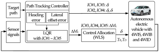
Figure 1.
Schematic diagram of the LQ path tracking controller.
This paper consists of five sections. In Section 2, a design procedure for the LQ path tracking controller with several input configurations is presented. In Section 3, performance measures for path tracking are presented. In Section 4, the simulation is shown, and the simulation results are analyzed in terms of the measures. The conclusion of this paper is given in Section 5.
2. Design of Path Tracking Controller with LQR
In this section, the state-space model was derived from 2-DOF bicycle and lateral offset and heading errors. With the model, LQR was designed with five input configurations given in Table 2. To convert the control yaw moment into tire forces for IC#3, IC#4, and IC#5, a weighted least square (WLS)-based method was adopted.
2.1. Design of LQR
For PTC, LQR was designed with the state-space equation derived from the lateral offset and heading errors. To obtain the state-space equation for PTC, a 2-DOF bicycle model was adopted. Figure 2 shows the coordinates and variables of the model and the target path used for path tracking [38]. For this model, it was assumed that the longitudinal velocity, vx, is constant. The equations of motions of the model are derived as Equation (1) with the state variables [34]. The slip angles of front and rear wheels, αf and αr, are defined as Equation (2). In Equation (1), the lateral tire forces of front and rear wheels, Fyf and Fyr, are assumed to be linear to αf and αr, as shown in Equation (3), respectively. In Equation (1), ΔMz is the control yaw moment needed for VSC and PTC. By combining Equations (1)–(3), the linear equations for the 2-DOF bicycle model were obtained as Equation (4).
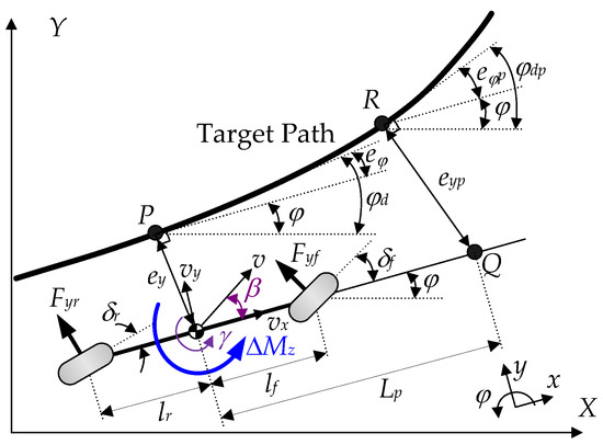
Figure 2.
Coordinates and variables of the 2-DOF bicycle model and target path.
In the literature of PTC, a lookahead or preview function is adopted to improve path tracking performance when deriving the lateral offset and heading errors [15,36,41,42,43,44,45]. Generally, the lateral offset and heading errors, ey and eφ, are defined at the point P in Figure 2. In this paper, lookahead distance Lp is calculated by Equation (5). Generally, kv is set between 1 and 2 s [41,44]. With Lp in Figure 2, the point Q is obtained along the heading of a vehicle. From the point Q, the point R is obtained on the target path along the perpendicular direction to the heading of the vehicle. In this paper, the lateral offset and heading errors are calculated at the point R.
Let the position of the center of gravity (CoG) of a vehicle be (x,y). The lateral offset and heading errors at the point P are defined as Equation (6). Those at the point R, i.e., eφp and eyp, are derived as Equation (6) [46,47,48]. As given in (6), if the heading error is smaller than 10°, sineφ and φdp can be approximated as eφ and φd, respectively. In this paper, kv is set to a particular value smaller than 0.1. If vx is smaller than 20 m/s, then the lookahead point Q is located near the center of the front axle, which is nearly the same as the Stanley method [44].
It is known that the derivative of the desired heading angle at the point P is defined as Equation (7), where χ is the curvature of the target path at the points R in Figure 2. From those definitions of Equations (6) and (7), the first- and second-derivatives of the lateral offset and heading errors at the point R are derived as those at the point P in Equation (8) [47]. With those variables, the state vector, x, and the disturbance, w, are defined as Equation (9).
According to available actuators in a vehicle, the control input u can be set as given in Table 1. As shown in Table 2, there are no additional actuators for path tracking for IC#1 and IC#2, except for FWS and 4WS. On the other hand, in IC#3, IC#4, and IC#5, the control yaw moment ΔMz can be converted into the steering angle at the rear wheels or the braking and traction torques at each wheel by a relevant yaw moment distribution procedure, where braking and traction torques are generated by 4WIB and 4WID, respectively. The front steering angle, δf, is available for all ICs. The rear steering angle, δr, is available for all ICs, except for IC#1, while 4WIB and 4WID are available for IC#3, IC#4, and IC#5. As mentioned earlier, the objective of this paper was to compare these input configurations in terms of path tracking performance.
From Equations (2), (3), (8), and (9) and Table 2, the state-space equation for path tracking is derived as Equation (10). In Equation (10), the input matrices for each input configuration, i.e., B2i, are given in Equation (11). In Equation (11), B2(i) represents the i-th column of the input matrix B2 of Equation (10).
The LQ objective functions for each input configuration are given in Equation (12). These functions can be converted into the vector-matrix form of (13). In (13), the matrices Q and Ri are obtained as Equation (14). In Equation (12), the weight ρi is determined by Bryson’s rule, as given in Equation (15). In Equation (15), ξi is the maximum allowable value of each term in Equation (12) [49]. For each input configuration, the control input ui of LQR is obtained as Equation (16), where Pi is the solution of the Riccati equation.
2.2. Control Allocation with the WLS-Based Method
Once ΔMz is obtained in IC#3, IC#4, and IC#5, it should be converted into lateral and longitudinal tire forces generated by actuators. The actuators used to generate the lateral tire forces are FWS/RWS, 4WS, and 4WIS. The actuators used to generate the longitudinal tire forces are 4WIB and 4WID. The procedure needed to convert ΔMz into the tire forces of each wheel is called control allocation or yaw moment distribution. For control allocation in this paper, a WLS-based method was adopted [12,14,15,16,17,25].
Figure 3 shows the coordinates of the tire forces and ΔMz, when ΔMz is positive [34]. The wheels in Figure 3 are numbered as 1, 2, 3, and 4 following the order of front left, front right, rear left, and rear right wheels. In Figure 3, ΔFx1 to ΔFx4 are the longitudinal tire forces generated by 4WIB and 4WID. If a longitudinal tire force is positive, then it is generated by 4WID. Otherwise, it is generated by 4WIB. Additionally, ΔFy1 to ΔFy4 stand for the lateral tire forces generated by FWS/RWS, 4WS, and 4WIS. Among them, ΔFy1 and ΔFy2 are generated by FWS, and ΔFy3 and ΔFy4 are generated by RWS or 4WS. To determine eight tire forces, the WLS-based method was used.
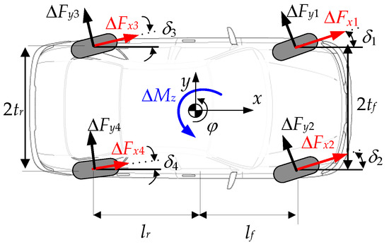
Figure 3.
The coordinate system corresponding to the tire forces and the control yaw moment.
From the geometrical relationship given in Figure 3, the force-moment equilibrium between ΔMz and tire forces is derived as Equation (17), where the elements of the vector g are calculated as Equation (18). In Equation (17), there are no constraints on the lateral forces, ΔFy1, ΔFy2, ΔFy3, and ΔFy4. As a result, the corresponding steering angles, δ1, δ2, δ3, and δ4, can be freely generated by 4WIS. For this reason, Equation (17) cannot represent the relationship between the tire forces and the corresponding steering angles imposed by RWS and 4WS. For RWS and 4WS, the steering angles of the front or rear wheels should be identical to each other, which is represented by the constraints, in Equation (19).
The objective function of WLS consists of two parts. The first part, JF, represents energy minimization, which is defined as Equation (20). In Equation (20), the radii of friction circles, μFzi, must be estimated. For the purpose in this paper, Fzi was estimated using longitudinal and lateral accelerations [50]. In Equation (20), κ is the vector of virtual weights, κi. κi serves to select the combination of each actuator [20,22]. The second part, JC, represents constraint satisfaction, which is defined as Equation (21). This is derived from Equation (17). In the previous study, Equation (17) should be satisfied in order to generate ΔMz. Under the condition, if ΔMz is large, then the lateral forces become much larger, which cannot be generated in real vehicles. To cope with this problem, the force-moment equilibrium Equation (17) is relaxed as Equation (21). By summing JF and JC with the tuning parameter η, the objective function JCA of WLS is obtained as Equation (22). In Equation (22), η is set to 1 or over it. Otherwise, the equality constraint, Equation (17), has no effect on JCA.
Generally, the friction circle constraints, as given in (23), are added in the optimization for VSC or PTC [33,50,51]. This is a nonlinear constraint, which causes a time-consuming iterative procedure to solve the constrained optimization problem. To avoid this, the friction circle constraint was not added to the optimization problem in this paper. Instead, the inverse of μFz in W takes the place of the friction circle constraint. The friction circle constraint can be used to measure the tire force margin (TFM), as given in Equation (24). If the TFM is small, the longitudinal and lateral tire forces approach its limits, which means an additional actuator used to generate these forces becomes less effective. As shown in Equation (24), TFM becomes much smaller under low μ conditions.
By differentiating Equation (22) with respect to q and setting it to zero, Equation (25) is obtained. By solving Equation (25), the optimum solution of Equation (22) is algebraically obtained as (26). Generally, quadratic programming with an equality constraint, Equation (27), can be easily solved as Equation (28) by applying the Lagrange multiplier technique [12,14,15,16,17,25,35]. If the constraint, Equation (19), is added when applying FWS, RWS, and 4WS, then the quadratic programming with the objective function, Equation (22), and the equality constraint, Equation (19), is obtained. By expanding and rearranging Equation (22), Equation (29) is obtained, which is equivalent to the objective function of Equation (27). Therefore, the optimum solution of Equation (22) with the constraint Equation (19) is algebraically obtained as Equation (28).
For each input configuration, available actuators are listed in Table 2. When applying WPCA for control allocation, corresponding actuators should be set for a particular input configuration. For this purpose, a set of virtual weights was used in this paper. Various actuator combinations of FWS, RWS, RWIS, 4WS, 4WIS, 4WIB, and 4WID needed to generate ΔMz can be selected by setting the virtual weights, κi [34,52]. As shown in Equation (17), the vector q has two parts, the lateral and longitudinal forces corresponding to the steering and braking/traction actuators. Thus, the virtual weights are set for the lateral and longitudinal forces. The vector of virtual weights corresponding to FWS, RWS, and 4WS/4WIS are given in Equations (30)–(32), respectively. In these equations, εi is a very small value, i.e., 10−4, compared to 1, and ● represents the virtual weights corresponding to the longitudinal tire forces of 4WIB and 4WID. In Equation (17), the first two and next two elements in q correspond to the front and rear wheels, respectively. Thus, Equation (30) represents the fact that the front wheel steering is available because ε1 and ε2 corresponding the front lateral forces are set to a very low value, i.e., 10−4. This makes the other lateral forces of qopt, i.e., ΔFy3 and ΔFy4, equal to zero. For the same reason, the virtual weights for RWS and 4WS/4WIS are set as Equations (31) and (32), respectively. It should be noted that the virtual weights of Equations (30)–(32) should be combined with the constraint, Equation (19), respectively. For example, if FWS is available, then Equations (19) and (30) are to be simultaneously used for optimization. Equation (19) guarantees that the front or rear steering angles are identical to each other, and Equation (30) guarantees that only the front lateral forces are generated by Equation (28).
The virtual weights corresponding to 4WIB and 4WID are given in Equations (33)–(35). Different from Equations (30)–(32), the longitudinal forces should be generated according to the direction of ΔMz. In these equations, εi is a very small value, i.e., 10−4, compared to 1, and ∗ represents the virtual weights corresponding to the lateral tire forces of FWS, RWS, and 4WIS. As shown in Figure 3, only ΔFx1 and ΔFx3 should be generated if 4WIB is available and ΔMz is positive. This is represented by Equation (33). If 4WIB and 4WID are available for generating ΔMz, then no constraints imposed on the longitudinal forces are needed, regardless of the direction of ΔMz. This is represented by Equation (35). The virtual weights given in Equations (30)–(35) can be set according to actuators available for generating ΔMz, as given in Table 2. For example, if 4WS/4WIS, 4WIB, and 4WID are available, then Equations (32) and (35) should be combined. In this case, all the elements in the vector of virtual weights, κ, have identical values. If 4WS is available, then Equation (32) should be imposed when solving Equation (26). As another example, Equations (31) and (34) should be combined if IC#3 in Table 2 is selected and RWS and 4WID are available.
Another usage of the virtual weights is to set the ratio between the tire forces of the vector q, as given in Equation (17) [31,34,52]. This is quite important when using rear-wheel steering in IC#2, IC#3, IC#4, and IC#5. When setting the weights ρi in the LQ objective function of Equation (12), the steering angles of the front and rear wheels become identical to each other if the weights on the heading error and its rate, i.e., ρ3 and ρ4 in Equation (12), are set to a very small value, compared to those on the lateral offset error. As a consequence, β becomes large, which can make a vehicle lose its lateral stability [14]. Moreover, ride comfort also deteriorates. There are three ways to cope with this problem. The first is to set higher weights on the heading error and its rate in Equation (12). The second is to set a bound on ΔMz for IC#3, IC#4, and IC#5. The third is to set the virtual weights of the rear steering angles, i.e., ε3 and ε4 in Equations (31) and (32), higher. As a result, ΔFx3 and ΔFx4 become smaller than ΔFx1 and ΔFx2 in qopt.
The tire force of each wheel determined by WLS, i.e., qopt in Equations (26) and (28), should be converted into a control input of each actuator. According to the sign of ΔFxi, the braking and traction torques, TBi and TBi, are calculated as Equations (36) and (37), respectively. In these equations, rwi, ωi, and ζi are the tire radius, the rotational speed, and the ratio of reduction gear at the i-th wheel, respectively. The function h(●) represents the capacity curve of an electric motor.
Different from the braking and traction torques, it is complex that the steering angles are determined from the lateral tire force ΔFyi obtained in qopt. In this paper, the steering angles were determined by using the definitions of the slip angle, Equation (2), and the linear lateral tire force, Equation (3). The linear lateral tire force, Equation (3), was rewritten as Equation (38). In Equation (38), σ is the parameter needed to tune the magnitude of the cornering stiffness, Ci. In fact, σ is equivalent to a slip ratio [36]. For 4WS, the steering angles of the front and rear wheels are calculated as Equation (39) by combining Equation (2) with Equation (38) [11]. However, this does not hold for 4WIS because the slip angle, Equation (2), is defined not for 4WIS but for 4WS. For 4WIS, the slip angles of each wheel are calculated as Equation (40) by using the geometrical relationship and vehicle dimensions as given in Figure 3. By combining Equation (38) with Equation (40), the steering angles of 4WIS are calculated as Equation (41) [30,34]. In these formulations, β should be measured or estimated. In this paper, the Kalman Filter-based method was adopted to estimate β [53].
3. Performance Measures for Path Tracking Control
To date, the lateral offset and heading errors have been used to evaluate path tracking performance. However, these measures can only represent the reachability of a controller. The responsiveness or agility of a controller should be evaluated for path tracking. For this reason, five measures for path tracking performance are presented in this paper [28].
In this paper, the target path is defined as Equation (42), which represents a double lane change maneuver for collision avoidance [11,13,14,18,19,20,22,23]. The target path is severe enough to evaluate the performance of path tracking controllers. Figure 4 shows the target path and vehicle trajectory, where the points A, B, and C are on the target path, and the points D, E, F, and G are on the vehicle trajectory. The target path can be divided into two step responses: the first is from the origin to the point A, and the second is from A to the destination. From those seven points on the paths, the following five measures are defined as Equation (43) to represent path tracking performance: the center offset ΔX, the lateral offset ΔY, the percentage over-shoot OS%, the response delay ΔDX, and the settling delay ΔSX, as depicted in Figure 4. In Equation (43), X(∗) and Y(∗) stand for the x- and y-positions of the point ∗, respectively.
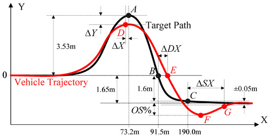
Figure 4.
Measures for path tracking performance.
The measures ΔX and ΔY stand for the agility and the reachability, respectively. If ΔX is negative, it means that the vehicle reached its peak, point D, early before target point A, as shown in Figure 4. In fact, ΔX can be regarded as a rising time to reach the peak. If ΔY is negative, it means that the first peak of the vehicle trajectory, Y(D), did not reach the target position, Y(A). In this paper, if ΔY is larger than −0.05 m, then the path tracking and collision avoidance performance of a controller are regarded as satisfactory.
OS% represents the damping along the lateral and yaw directions, which represents the agility. As shown in Figure 4, the y-position of the centerline of the lower lane is −1.65 m. If the tread of the vehicle is 1.6m and Y(F) is larger than −2.5 m, then the vehicle remains inside the lower lane, which means that the maximum allowable overshoot is 0.85 m. The overshoot of 0.85 m is calculated as 16%, as given in Equation (43). For this reason, it is regarded as acceptable if OS% is less than 16%.
ΔDX is the response delay, which stands for the response speed of the vehicle motion in path tracking. ΔSX is the settling delay, equivalent to the settling time in control theory. ΔSX stands for how fast the vehicle motion converges to a particular range around a target value. When calculating ΔSX, a ±0.05 m range around −1.65 m was set in this paper. If the CoG of the vehicle converges to the range of −1.65 ± 0.05 m, then the vehicle trajectory is considered converged.
Generally, lateral stability is represented by β. In real vehicles, lateral stability is considered maintained if β is controlled not to exceed 3° [31]. Generally, the smaller β the better. In this paper, the maximum absolute value of the side-slip angle is denoted as MASSA.
4. Simulation and Validation
A simulation was performed to compare the performance of the input configurations of an LQ path tracking controller on low μ roads. The controllers were implemented with MATLAB/Simulink, and the simulation was run in a co-simulation environment with MATLAB/Simulink and CarSim [54]. The test scenario was path tracking on the target path, Equation (42). For the simulation, the F-segment sedan model in CarSim was selected [54]. This model is a 27-DOF nonlinear one including a single sprung mass, four wheels, four suspensions with nonlinear springs and dampers, and a steering mechanism. The configurations of suspensions in this model were front and rear independent axles. From the model, the parameters and its values of the 2-DOF bicycle model are referred to as given in Table 3. The position and heading information and dynamic variables such as velocities and tire forces were directly read from CarSim. For a realistic simulation, a sensor noise reflecting real sensors on real vehicles can be added to the signals obtained from CarSim. However, it was not considered in this paper because the aim of this paper was to compare the input configurations of LQ path tracking controllers. The comparison can be conducted without realistic assumptions on sensors and actuators. The control inputs calculated in MATLAB/Simulink are directly fed to CarSim. The realistic behavior of an actuator was modelled with first-order system with a particular time constant. In this paper, the steering actuators, FWS, RWS, RWIS, 4WS, and 4WIS, and the braking and driving actuators, 4WIB and 4WID, were modelled as the first-order systems with time constants of 0.02 and 0.01, respectively. The initial vx and μ were set to 60 km/h and 0.4, respectively. In order to keep the vehicle speed constant, a built-in speed controller provided in CarSim was applied.
Table 3.
Parameters and values from the F-segment sedan model in CarSim.
As mentioned earlier, it is necessary to set a bound on ΔMz in order to make the rear steering angle small for IC#3, IC#4, and IC#5. For this purpose, ΔMz was limited to a certain value. This was performed after ΔMz was obtained from LQR. For IC#3 and IC#4, the maximum of ΔMz was limited to 2000 Nm [11]. The maximum lateral tire force from the F-segment sedan model in CarSim is 7500 N if μ is 1. This was 3000 N for this paper because μ was set to 0.4. From Table 2, the maximum available yaw moment was calculated as 3000 × 2 × (lf + lr) = 18,000 Nm. Thus, the maximum of ΔMz was limited to 18,000 Nm for IC#5, in this paper. The maximum steering angles of the front and rear wheels were set to 30°.
The first simulation was performed for IC#1 and IC#2, which were used as a baseline for comparison to the others. Table 4 shows the parameters and gain elements of the controllers, which were tuned such that ΔY was larger than −0.05 m. In Table 4, ξ is the vector of the maximum allowable values, as given in Equation (15).
Table 4.
The set of parameters used for each controller.
Figure 5 and Figure 6 show the simulation results for IC#1 and IC#2. Table 5 summarizes those results. As shown in Figure 5 and Figure 6, the LQRs with IC#1 and IC#2 gave nearly identical results and showed satisfactory path tracing performance on low μ roads. The side-slip angles of these controllers were kept as small and nearly identical to one another in spite of the low μ condition. This means that lateral stability was maintained well by the path tracking controllers. In the case of IC#3, this was caused by the small rear steering angles, as given in Figure 5a. As shown in Figure 5c, the side-slip angles of IC#1 and IC#2 were less than 1°, which means that lateral stability was maintained well.
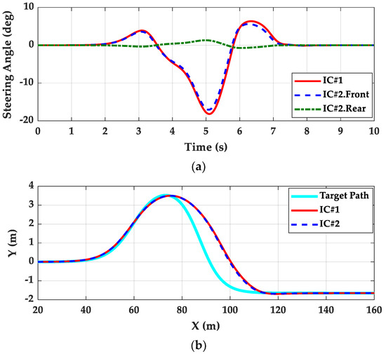
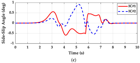
Figure 5.
Simulation results for IC#1 and IC#2: (a) steering angles, (b) trajectories, (c) side–slip angles.
Figure 6.
Simulation results of tire forces for IC#1 and IC#2: (a) slip angles vs. lateral tire forces, (b) tire force margin.
Table 5.
Summary of the simulation results for IC#1 and IC#2.
Figure 6 shows the simulation results of tire forces for IC#1 and IC#2. In Figure 6, FL, FR, RL, and RR stand for front left, front left, rear left, and rear left wheels, respectively. As shown in Figure 6a, the lateral tire forces of IC#1 and IC#2 were saturated regardless of front or rear wheels. This was caused by the low μ condition, which means that the available lateral tire force for the control became small. As a result of this, the TFMs became small, which is shown in Figure 6b. This means that additional actuators such as 4WIB and 4WID became less effective when improving path tracking performance. Moreover, this also means that LQR with IC#2 gave the best path tracking performance regardless of the use of 4WID and 4WIB.
As shown in Table 5, the LQRs with IC#1 and IC#2 gave nearly similar results except for MASSA. The LQR with IC#2 slightly improved path tracking performance by virtue of RWS, compared to LQR with IC#1. Among the measures, ΔX, ΔY, and OS% can be improved by tuning the weights in the LQ objective function. Instead, ΔDX and ΔSX will deteriorate. ΔDX given in Table 2 is the minimum achievable by LQR under the condition that μ is 0.4. In other words, ΔDX cannot be improved by any additional actuators or tuning on the weights.
From these results, it can be concluded that lateral stability can be kept on low μ roads without any schemes coordinating path tracking and lateral stability. In addition to this, it can be also concluded that additional actuators are not needed to improve path tracking performance or to keep lateral stability small on low μ roads due to a small tire force margin.
The second simulation was conducted for IC#3 and IC#4. In this simulation, the WLS-based control allocation was applied to distribute ΔMz to the longitudinal and lateral tire forces. Table 6 and Table 7 show the parameters and gain elements of the controllers with IC#3 and IC#4, respectively, which were tuned such that ΔY was larger than −0.05 m. The maximum steering angles of the front and rear wheels were set to 30°. As mentioned earlier, the maximum ΔMz was limited to 2000 Nm.
Table 6.
The set of parameters used for IC#3.
Table 7.
The set of parameters used for IC#4.
Table 8 and Table 9 summarize the simulation results for IC#3 and IC#4, respectively. For IC#3 and IC#4, eight and three actuator combinations were used to generate ΔMz, respectively. As shown in Table 5 and Table 8, there are also little differences between IC#1 and the first three rows of Table 8. This means that FWS itself was enough for path tracking on low μ roads without any additional actuators. As shown in Table 8 and Table 9, there are also little meaningful differences among measures for the LQRs with IC#3 and IC#4. This means that FWS or 4WS itself has a large effect on path tracking performance. As a result, there is a small tire force margin to improve the performance, as shown in Figure 6b. Moreover, those actuator combinations used a relatively small ΔMz within the given limit, as shown in the last column of Table 8 and Table 9, Max.|ΔMz|. Even though ΔMz was saturated to 2000Nm, the controllers showed good path tracking performance. These results confirm that additional actuators to FWS or 4WS are not effective due to the small tire force margin.
Table 8.
Summary of the simulation results for IC#3.
Table 9.
Summary of the simulation results for IC#4.
The third simulation was conducted for IC#5. As in the case of IC#3 and IC#4, the WLS-based control allocation was applied to distribute ΔMz to the longitudinal and lateral tire forces. Moreover, there were no FWS or 4WS in IC#5. Table 10 shows the parameters and gain elements of the controllers, which were tuned such that ΔY was larger than −0.05 m. The maximum steering angles of the front and rear wheels were set to 30°. As mentioned earlier, the maximum ΔMz was limited to 18,000 Nm. In this case, the virtual weights on the rear steering wheels were set higher because it was necessary to limit the rear steering angles in order to keep β as small as possible. The vectors of virtual weights for each actuator combination are given in Table 10.
Table 10.
The set of parameters used for IC#5.
Table 11 summarizes the simulation results for IC#5. As shown in Table 11, three types of steering actuators, i.e., FWS, 4WS, and 4WIS, were adopted for IC#5. For each steering actuator, 4WID and 4WIB were combined. As a result, twelve actuator combinations were used to generate ΔMz. As shown in Table 11, there are little meaningful differences between actuator combinations. A notable feature of IC#5 is that all the measures were slightly improved by several actuator combinations used for control allocation. ΔX was clearly improved for all actuator combinations. For example, using only FWS to generate ΔMz for IC#5 showed better ΔX than IC#1 by comparing the first rows of Table 5 and Table 11. However, every actuator combination except FWS and 4WS in IC#5 needed more than two actuators to generate ΔMz. Moreover, they require a tedious and time-consuming tuning process on several parameters and weights of the controllers, compared to IC#1 and IC#2. To sum up the above results, it can be concluded that the LQR with IC#1 or IC#2 was quite effective enough, and no additional actuators are not needed for path tracking on low μ roads.
Table 11.
Summary of the simulation results for IC#5.
5. Conclusions
The aim of this paper was to compare path tracking performance among the input configurations of LQR and available actuators for each input configuration in low-friction conditions in a single framework. For this purpose, the five input configurations were identified from a literature survey. With those input configurations, the LQR was designed with the state-space model derived from the bicycle model and a target path. To convert the control yaw moment in the input configurations, the WLS-based method was adopted. In this procedure, the virtual weights and equality constraints were introduced to represent several actuator combinations such as 4WS, RWIS, 4WIS, 4WID, and 4WIB needed to generate the control yaw moment. To analyze the path tracking performance of the input configurations of LQR, simulations were performed in a vehicle simulation package, CarSim. From the simulation results, it was shown that FWS or 4WS is enough for path tracking on low μ roads, and no additional actuators were required to improve path tracking performance. This fact also holds for SMC and MPC if these adopt the identical input configurations of LQR. The most critical problem when designing LQR for path tracking is to tune the weights in the LQ objective function under parameter variations. This requires the design of a robust and non-fragile controller that can guarantee path tracking performance under variations of parameters and gain elements.
Author Contributions
M.P. conceptualized the main idea and designed this study. S.Y. participated in formulating the idea, as well as validating the proposed method and results. S.Y. implemented the methodology and drafted the manuscript. All authors have read and agreed to the published version of the manuscript.
Funding
This work was supported by the Ministry of Trade, Industry and Energy (MOTIE, Korea) (No. 20018055, Development of fail operation technology in Lv.4 autonomous driving systems). This work is also supported by the Korea Agency for Infrastructure Technology Advancement (KAIA) grant funded by the Ministry of Land, Infrastructure and Transport (grant no. 22AMDPC160501-03).
Institutional Review Board Statement
Not applicable.
Informed Consent Statement
Not applicable.
Data Availability Statement
Not applicable.
Conflicts of Interest
The authors declare no conflict of interest.
Nomenclature
| 4WS | 4-wheel steering |
| 4WIS | 4-wheel independent steering |
| 4WIB | 4-wheel independent braking |
| 4WID | 4-wheel independent drive |
| AFS | active front steering |
| FWS | front wheel steering |
| MASSA | maximum absolute side-slip angle |
| RWS | rear wheel steering |
| RWIS | rear wheel independent steering |
| TFM | tire force margin |
| WLS | weighted least square |
| Cf, Cr | cornering stiffness of front and rear tires (N/rad) |
| Ci | cornering stiffness of i-th wheel (N/rad) |
| ey, eφ | lateral offset error (m) and heading error (rad) |
| eyp, eφp | lateral offset error (m) and heading error (rad) obtained from lookahead |
| Fxi, Fyi, Fzi | longitudinal, lateral, and vertical tire forces of i-th wheel (N) |
| Fyf, Fyr | front and rear lateral tire forces in the 2-DOF bicycle model (N) |
| g | vector used for the equality constraint in WLS-based method |
| h() | capacity curve of an electric motor |
| H | matrix used for the constraint on RWS and 4WS in the WLS-based method |
| Iz | yaw moment of inertial (kg·m2) |
| Ji | LQ objective function for the input configuration IC#i |
| KLQR,i | gain matrix of LQR for input configuration IC#i |
| kv | velocity gain for lookahead distance |
| Lp | lookahead distance (m) |
| lf, lr | distance from CoG to front and rear axles (m) |
| m | vehicle total mass (kg) |
| OS% | percentage of overshoot in the lower lane of the target path |
| q | vector of tire forces as a solution to the WLS-based method |
| rwi | radius of i-th wheel (m) |
| TBi, TDi | braking and traction torques applied at i-th wheel (N·m) |
| tf, tr | half of track widths of front and rear axles (m) |
| vx, vy | longitudinal and lateral velocities of CoG of a vehicle (m/s) |
| W | weighting matrix of the WLS-based method |
| X(∗), Y(∗) | x- and y-positions of the point ∗ on the target path and vehicle trajectory |
| Yref(X) | y-position of the target path with respect to X |
| y | lateral offset of a vehicle |
| yd, ydp | desired lateral offset obtained without and with lookahead |
| αf, αr | tire slip angles of front and rear wheels (rad) |
| αi | tire slip angle of i-th wheel (rad) |
| β | side-slip angle of CoG of a vehicle (rad) = tan−1(vy/vx) ≈ (vy/vx) |
| δf, δr | front and rear steering angles (rad) |
| δi | steering angle of i-th wheel (rad) |
| εi | virtual weights on corresponding lateral and longitudinal tire forces |
| ΔFxi, ΔFyi | control longitudinal and lateral forces generated by an actuator (N) |
| ΔFx | longitudinal force as a control input in LQR (N) |
| ΔMz | control yaw moment as a control input in LQR (N·m) |
| ΔX, ΔY | differences between x- and y-positions at the peak points of the target path |
| ΔDX, ΔSX | response and settling delays of vehicle trajectory with respect to target path |
| γ, γd | real and reference yaw rates (rad/s) |
| η | tuning parameter on relaxation term of equality constraint |
| χ | curvature at a particular point on a target path |
| κ | virtual weight on the longitudinal and lateral tire forces |
| κ | vector of virtual weights |
| ξi | the maximum allowable value of i-th term in LQ objective function |
| ξ | vector of the maximum allowable values |
| ϕi | equivalent slip angle of i-th wheel calculated from control lateral tire force |
| φ | heading angle of a vehicle |
| φd, φdp | desired heading angle obtained without and with lookahead |
| ψref(χ) | heading angle of the target path with respect to X |
| μ | tire-road friction coefficient |
| ωi | rotational speed of i-th wheel (rad/s) |
| ρi | weight on i-th term in LQ objective function |
| σ | equivalent slip ratio for slip angle calculation |
| ζi | ratio of reduction gear of i-th wheel |
References
- Montanaro, U.; Dixit, S.; Fallaha, S.; Dianatib, M.; Stevensc, A.; Oxtobyd, D.; Mouzakitisd, A. Towards connected autonomous driving: Review of use-cases. Veh. Syst. Dyn. 2019, 57, 779–814. [Google Scholar] [CrossRef]
- Yurtsever, E.; Lambert, J.; Carballo, A.; Takeda, K. A survey of autonomous driving: Common practices and emerging technologies. IEEE Access 2020, 8, 58443–58469. [Google Scholar] [CrossRef]
- Omeiza, D.; Webb, H.; Jirotka, M.; Kunze, M. Explanations in autonomous driving: A survey. IEEE Trans. Intell. Transp. Syst. 2022, 23, 10142–10162. [Google Scholar] [CrossRef]
- Sorniotti, A.; Barber, P.; De Pinto, S. Path tracking for automated driving: A tutorial on control system formulations and ongoing research. In Automated Driving; Watzenig, D., Horn, M., Eds.; Springer: Cham, Switzerland, 2017. [Google Scholar]
- Amer, N.H.; Hudha, H.Z.K.; Kadir, Z.A. Modelling and control strategies in path tracking control for autonomous ground vehicles: A review of state of the art and challenges. J. Intell. Robot. Syst. 2017, 86, 225–254. [Google Scholar] [CrossRef]
- Paden, B.; Cap, M.; Yong, S.Z.; Yershov, D.; Frazzoli, E. A survey of motion planning and control techniques for self-driving urban vehicles. IEEE Trans. Intell. Veh. 2016, 1, 33–55. [Google Scholar] [CrossRef]
- Bai, G.; Meng, Y.; Liu, L.; Luo, W.; Gu, Q.; Liu, L. Review and comparison of path tracking based on model predictive control. Electronics 2019, 8, 1077. [Google Scholar] [CrossRef]
- Yao, Q.; Tian, Y.; Wang, Q.; Wang, S. Control strategies on path tracking for autonomous vehicle: State of the art and future challenges. IEEE Access 2020, 8, 161211–161222. [Google Scholar] [CrossRef]
- Rokonuzzaman, M.; Mohajer, N.; Nahavandi, S.; Mohamed, S. Review and performance evaluation of path tracking controllers of autonomous vehicles. IET Intell. Transp. Syst. 2021, 15, 646–670. [Google Scholar] [CrossRef]
- Stano, P.; Montanaro, U.; Tavernini, D.; Tufo, M.; Fiengo, G.; Novella, L.; Sorniotti, A. Model predictive path tracking control for automated road vehicles: A review. Annu. Rev. Control. 2022. [Google Scholar] [CrossRef]
- Yakub, F.; Mori, Y. Comparative study of autonomous path-following vehicle control via model predictive control and linear quadratic control. Proc. IMechE Part D J. Automob. Eng. 2015, 229, 1695–1714. [Google Scholar] [CrossRef]
- Hu, C.; Wang, R.; Yan, F.; Chen, N. Output constraint control on path following of four-wheel independently actuated autonomous ground vehicles. IEEE Trans Veh. Technol. 2016, 65, 4033–4043. [Google Scholar] [CrossRef]
- Hang, P.; Luo, F.; Fang, S.; Chen, X. Path tracking control of a four-wheel-independent-steering electric vehicle based on model predictive control. In Proceedings of the 2017 36th Chinese Control Conference (CCC), Dalian, China, 26–28 July 2017. [Google Scholar]
- Hang, P.; Chen, X.; Luo, F. Path-tracking controller design for a 4WIS and 4WID electric vehicle with steer-by-wire system. SAE Tech. Pap. 2017, 2688–3627.
- Guo, J.; Luo, Y.; Li, K. An adaptive hierarchical trajectory following control approach of autonomous four-wheel independent drive electric vehicles. IEEE Trans Intell. Transp. Syst. 2018, 19, 2482–2492. [Google Scholar] [CrossRef]
- Hang, P.; Chen, X.; Luo, F. LPV/H∞ controller design for path tracking of autonomous ground vehicles through four-wheel steering and direct yaw-moment control. Int. J. Automot. Technol. 2019, 20, 679–691. [Google Scholar] [CrossRef]
- Ren, Y.; Zheng, L.; Khajepour, A. Integrated model predictive and torque vectoring control for path tracking of 4-wheeldriven autonomous vehicles. IET Intell. Transp. Syst. 2019, 13, 98–107. [Google Scholar] [CrossRef]
- Chen, X.; Peng, Y.; Hang, P.; Tang, T. Path tracking control of four-wheel independent steering electric vehicles based on optimal control. In Proceedings of the 2020 39th Chinese Control Conference (CCC), Shenyang, China, 27–29 July 2020; pp. 5436–5442. [Google Scholar]
- Wu, H.; Si, Z.; Li, Z. Trajectory tracking control for four-wheel independent drive intelligent vehicle based on model predictive control. IEEE Access 2020, 8, 73071–73081. [Google Scholar] [CrossRef]
- Wu, H.; Li, Z.; Si, Z. Trajectory tracking control for four-wheel independent drive intelligent vehicle based on model predictive control and sliding mode control. Adv. Mech. Eng. 2021, 13, 1–17. [Google Scholar] [CrossRef]
- Hang, P.; Chen, X. Path tracking control of 4-wheelsteering autonomous ground vehicles based on linear parameter-varying system with experimental verification. Proc. IMechE Part I J. Syst. Control. Eng. 2021, 235, 411–423. [Google Scholar]
- Xiang, C.; Peng, H.; Wang, W.; Li, L.; An, Q.; Cheng, S. Path tracking coordinated control strategy for autonomous four in-wheel-motor independent-drive vehicles with consideration of lateral stability. Proc. IMechE Part D J. Automob. Eng. 2021, 235, 1023–1036. [Google Scholar] [CrossRef]
- Yang, K.; Tang, X.; Qin, Y.; Huang, Y.; Wang, H.; Pu, H. Comparative study of trajectory tracking control for automated vehicles via model predictive control and robust H-infinity state feedback control. Chin. J. Mech. Eng. 2021, 34, 1–14. [Google Scholar] [CrossRef]
- Wang, G.; Liu, L.; Meng, Y.; Gu, Q.; Bai, G. Integrated path tracking control of steering and braking based on holistic MPC. IFAC Pap. 2021, 54, 45–50. [Google Scholar] [CrossRef]
- Barari, A.; Afshari, S.S.; Liang, X. Coordinated control for path-following of an autonomous four in-wheel motor drive electric vehicle. Proc. IMechE Part C J. Mech. Eng. Sci. 2022, 236, 6335–6346. [Google Scholar] [CrossRef]
- Wang, G.; Liu, L.; Meng, Y.; Gu, Q.; Bai, G. Integrated path tracking control of steering and differential braking based on tire force distribution. Int. J. Control. Autom. Syst. 2022, 20, 536–550. [Google Scholar] [CrossRef]
- Wang, W.; Zhang, Y.; Yang, C.; Qie, T.; Ma, M. Adaptive model predictive control-based path Following control for four-wheel independent drive automated vehicles. IEEE Trans. Intell. Transp. Syst. 2022, 23, 14399–14412. [Google Scholar] [CrossRef]
- Lee, J.; Yim, S. Comparative study of path tracking controllers on low friction roads for autonomous vehicles. Machines. 2023, 11, 403. [Google Scholar] [CrossRef]
- Du, Q.; Zhu, C.; Li, Q.; Tian, B.; Li, L. Optimal path tracking control for intelligent four-wheel steering vehicles based on MPC and state estimation. Proc. IMechE Part D J. Automob. Eng. 2022, 236, 1964–1976. [Google Scholar] [CrossRef]
- Jeong, Y.; Yim, S. Path tracking control with four-wheel independent steering, driving and braking systems for autonomous electric vehicles. IEEE Access 2022, 10, 74733–74746. [Google Scholar] [CrossRef]
- Yim, S. Coordinated control with electronic stability control and active steering devices. J. Mech. Sci. Technol. 2015, 29, 5409–5416. [Google Scholar] [CrossRef]
- Yim, S. Comparison among active front, front independent, 4-wheel and 4-wheel independent steering systems for vehicle stability control. Electronics 2020, 9, 798. [Google Scholar] [CrossRef]
- Wang, J.; Wang, R.; Jing, H.; Chen, N. Coordinated active steering and four-wheel independently driving/braking control with control allocation. Asian J. Control. 2016, 18, 98–111. [Google Scholar] [CrossRef]
- Nah, J.; Yim, S. Vehicle stability control with four-wheel independent braking, drive and steering on in-wheel motor-driven electric vehicles. Electronics 2020, 9, 1934. [Google Scholar] [CrossRef]
- Katsuyama, E.; Yamakado, M.; Abe, M. A state-of-the art review: Toward a novel vehicle dynamics control concept taking the driveline of electric vehicles into account as promising control actuators. Veh. Syst. Dyn. 2021, 59, 976–1025. [Google Scholar] [CrossRef]
- Liang, Y.; Li, Y.; Zheng, L.; Yu, Y.; Ren, Y. Yaw rate tracking-based path-following control for four-wheel independent driving and four-wheel independent steering autonomous vehicles considering the coordination with dynamics stability. Proc. IMechE Part D J. Automob. Eng. 2021, 235, 260–272. [Google Scholar] [CrossRef]
- Wong, H.Y. Theory of Ground Vehicles, 3rd ed.; John Wiley and Sons Inc.: New York, NY, USA, 2001. [Google Scholar]
- Rajamani, R. Vehicle Dynamics and Control; Springer: New York, NY, USA, 2006. [Google Scholar]
- Guo, J.; Luo, Y.; Li, K.; Dai, Y. Coordinated path-following and direct yaw-moment control of autonomous electric vehicles with sideslip angle estimation. Mech. Syst. Signal Process. 2018, 105, 183–199. [Google Scholar] [CrossRef]
- Peng, H.; Wang, W.; An, Q.; Xiang, C.; Li, L. Path tracking and direct yaw moment coordinated control based on robust MPC with the finite time horizon for autonomous independent-drive vehicles. IEEE Trans. Veh. Technol. 2020, 69, 6053–6066. [Google Scholar] [CrossRef]
- Sharp, R.S.; Casanova, D.; Symonds, P. A mathematical model for driver steering control, with design, tuning and performance results. Veh. Syst. Dyn. 2000, 33, 289–326. [Google Scholar]
- Thommyppillai, M.; Evangelou, S.; Sharp, R.S. Advances in the development of a virtual car driver. Multibody Syst. Dyn. 2009, 22, 245–267. [Google Scholar]
- Xu, S.; Peng, H. Design, analysis and experiments of preview path tracking control for autonomous vehicles. IEEE Trans. Intell. Transp. Syst. 2020, 21, 48–58. [Google Scholar] [CrossRef]
- Thrun, S.; Montemerlo, M.; Dahlkamp, H.; Stavens, D.; Aron, A.; Diebel, J.; Fong, P.; Gale, J.; Halpenny, M.; Hoffmann, G.; et al. Stanley: The robot that won the DARPA grand challenge. J. Field Robot. 2006, 23, 661–692. [Google Scholar] [CrossRef]
- Son, Y.S.; Kim, W.; Lee, S.-H.; Chung, C.C. Robust multi-rate control scheme with predictive virtual lanes for lane-keeping system of autonomous highway driving. IEEE Trans. Veh. Technol. 2015, 64, 3378–3391. [Google Scholar] [CrossRef]
- Kang, C.M.; Lee, S.-H.; Chung, C.C. On-road path generation and control for waypoint tracking. IEEE Intell. Transp. Syst. Mag. 2016, 9, 36–45. [Google Scholar] [CrossRef]
- Kim, D.J.; Kang, C.M.; Lee, S.H.; Chung, C.C. Discrete-time integral sliding model predictive control for dynamic lateral motion of autonomous driving vehicles. In Proceedings of the American Control Conference, Washington, DC, USA, 17–19 June 2018; pp. 4757–4763. [Google Scholar]
- Lee, K.; Jeon, S.; Kim, H.; Kum, D. Optimal path tracking control of autonomous vehicle: Adaptive full-state linear quadratic gaussian (LQG) control. IEEE Access 2019, 7, 109120–109133. [Google Scholar] [CrossRef]
- Bryson, A.E.; Ho, Y.C. Applied Optimal Control; Hemisphere: New York, NY, USA, 1975. [Google Scholar]
- Rezaeian, A.; Zarringhalam, R.; Fallah, S.; Melek, W.; Khajepour, A.; Chen, S.-K.; Moshchuck, N.; Litkouhi, B. Novel tire force estimation strategy for real-time implementation on vehicle applications. IEEE Trans. Veh. Technol. 2015, 64, 2231–2241. [Google Scholar] [CrossRef]
- de Castro, R.; Tanelli, M.; Araújo, R.E.; Savaresi, S.M. Design of safety-oriented control allocation strategies for overactuated electric vehicles. Veh. Syst. Dyn. 2014, 52, 1017–1046. [Google Scholar] [CrossRef]
- Yim, S.; Choi, J.; Yi, K. Coordinated control of hybrid 4WD vehicles for enhanced maneuverability and lateral stability. IEEE Trans. Veh. Technol. 2012, 61, 1946–1950. [Google Scholar] [CrossRef]
- Kim, H.H.; Ryu, J. Sideslip angle estimation considering short-duration longitudinal velocity variation. Int. J. Automot. Technol. 2011, 12, 545–553. [Google Scholar] [CrossRef]
- Mechanical Simulation Corporation. VS Browser: Reference Manual, The Graphical User Interfaces of BikeSim, CarSim, and TruckSim; Mechanical Simulation Corporation: Ann Arbor, MI, USA, 2009. [Google Scholar]
Disclaimer/Publisher’s Note: The statements, opinions and data contained in all publications are solely those of the individual author(s) and contributor(s) and not of MDPI and/or the editor(s). MDPI and/or the editor(s) disclaim responsibility for any injury to people or property resulting from any ideas, methods, instructions or products referred to in the content. |
© 2023 by the authors. Licensee MDPI, Basel, Switzerland. This article is an open access article distributed under the terms and conditions of the Creative Commons Attribution (CC BY) license (https://creativecommons.org/licenses/by/4.0/).