Article

Transfer Learning-Based Fault Diagnosis Method for Marine Turbochargers

1
School of Naval Architecture, Ocean and Energy Power Engineering, Wuhan University of Technology, Wuhan 430063, China
2
National Engineering Laboratory for Marine and Ocean Engineering Power System, Electronic Control Sub-Laboratory for Low-Speed Engine, Wuhan 430063, China
3
Key Laboratory of Marine Power Engineering and Technology Granted by MOT, Wuhan 430063, China
*
Author to whom correspondence should be addressed.
Actuators 2023, 12(4), 146; https://doi.org/10.3390/act12040146
Submission received: 7 March 2023 / Revised: 26 March 2023 / Accepted: 27 March 2023 / Published: 28 March 2023
(This article belongs to the Section Control Systems)

Abstract

:
To address the issues of the high cost of marine turbocharger fault simulation testing and the difficulties in obtaining fault sample data, a multi-body dynamics model of a marine turbocharger was developed. The simulation approach was used to acquire the turbocharger vibration signals. The result shows that the amplitude of the 1× vibration signal power spectrum drops as the bearing surface roughness increases. However, the amplitude of the 2× and 9× vibration signal power spectra increases as the roughness increases. The TrAdaBoost transfer learning method is used to develop a marine turbocharger diagnosis model. The validation results of 2040 simulated fault samples reveal that when the desired sample number is 20, the diagnostic model has an accuracy of 87%. When the desired number of samples is 40, the diagnostic model’s accuracy is 96%. The diagnosis model may perform diagnosis information transfer between the actual turbocharger and the simulation model.

1. Introduction

The turbocharger is a crucial component of a marine diesel engine [1]. Among all diesel engine components, it is the most prone to damage. The turbocharger has a considerable influence on diesel engine performance once it breaks [2,3]. Furthermore, due to the intense working environment and complicated composition system of marine turbochargers, they are prone to problems during operation [4]. A substantial quantity of failure sample data is required for the quick and accurate diagnosis of marine turbocharger failures. However, the economic cost and danger of failure test are also great. The purpose of the model-based fault simulation study is to simulate the common types of turbocharger failures in actual operation using professional simulation software. Fault simulation greatly reduces the time and economic cost required for fault data acquisition. Meanwhile, it also provides rich sample data for fault diagnosis and turbocharger health status monitoring.
In turbocharger rotor dynamics simulation studies, Li was the first to apply a bearing finite element model to predict the steady-state response of oil film [5]. Peixoto et al. developed a turbocharger rotor dynamic model, accounting for lateral and axial vibrations and cross-coupling bearing effects, to analyze run down or run up dynamic response. Predictions show a fair agreement with test data in the frequency domain and temperature estimates, especially for higher rotational speeds [6]. Ntonas et al. present a turbocharged four-stroke diesel engine simulation framework based on one-dimensional calculations and analysis. Mean-line models were used in conjunction with the beta lines method for generating accurate and detailed compressor and turbine performance maps [7]. Koutsovasilis et al. investigate the influence of hydrodynamic thrust bearings on the nonlinear oscillations and bifurcations of the rotor system in terms of the thrust and radial bearing interaction during run-ups. For a given set of boundaries, the thrust bearing’s position along the shaft can have either positive, neutral or negative influence on shaft motion [8]. Wang et al. established a rotor system dynamics simulation model with an improved four-node aggregate parameter method. A fault simulation was performed. The output fault simulation signal is extracted by the Hu-invariant moment feature extraction method [9]. Bin et al. developed a finite element model of a turbocharger rotor and analyzed the nonlinear dynamic response of the rotor. It was found that rotor unevenness has an important effect on subsynchronous vibrations [10].
Fault diagnosis methods for marine diesel engine turbochargers are divided into two main categories: model-based methods and data-driven methods. The model-based fault diagnosis method is common and widely used. It uses physical signals such as temperature, pressure and vibration, as well as equipment-related mechanistic knowledge for modelling [11,12,13,14,15]. However, the mathematical model of the marine turbocharger is complex and cannot be accurately modelled due to its nonlinear characteristics, system uncertainty, external disturbances and changes in operating conditions. Therefore, data-driven fault diagnosis methods based on real-time health condition monitoring are increasingly used [16,17,18,19,20,21]. Multivariate statistical analysis methods, subspace identification methods and pattern recognition methods have been well applied in model identification and can be widely used in complex industrial systems, for example, partial least squares (PLS), typical correlation analysis (CCA), efficient projection to latent structures (EPLS), fault trees and machine learning [22,23,24,25,26]. At the same time, the effectiveness of the above methods is strongly influenced by the quality of the data. Therefore, it is necessary to apply a combination of both methods.
Traditional machine learning-based algorithms require a large amount of data for training. However, they also require that the training and test data are independently and identically distributed [27,28]. Meanwhile, in practice, factors such as the speed, health status, ambient temperature and altitude of the turbocharger can affect the independent, identical distribution of the data. The TrAdaBoost transfer learning algorithm can solve the problem of the independent identical distribution of the data and transfer knowledge between different but similar domains. Additionally, only a small amount of fault sample data plus some auxiliary data are needed to classify the data [29,30]. Then, simulation or other means can be used to obtain a large amount of auxiliary data. Finally, a small amount of independent identically distributed fault sample data is easy to obtain.
In this paper, a multi-body dynamics model of a marine turbocharger was established based on AVL Excite software. Its simulation calculation results were analyzed. The tests were carried out on the bench, and the simulation and test results were compared to ensure that the model was accurate. The model’s inaccuracy is less than 5%. Then, the approach of turbocharger dynamics fault simulation was validated. Based on the model, fault simulation and data analysis were carried out. The amplitude of the 1× vibration signal power spectrum drops as the bearing surface roughness increases. However, the amplitude of the 2× and 9× vibration signal power spectra increases as the roughness increases. A defect diagnostic model for marine diesel engine turbocharger system is built using the TrAdaBoost algorithm. The diagnostic model has a 96% accuracy rate. The diagnosis findings indicate that the algorithm can transfer diagnostic knowledge between the real engine and the simulation model of a marine turbocharger. It provides a new way of thinking about turbocharger failure diagnosis.

2. Turbocharger Simulation Model Building

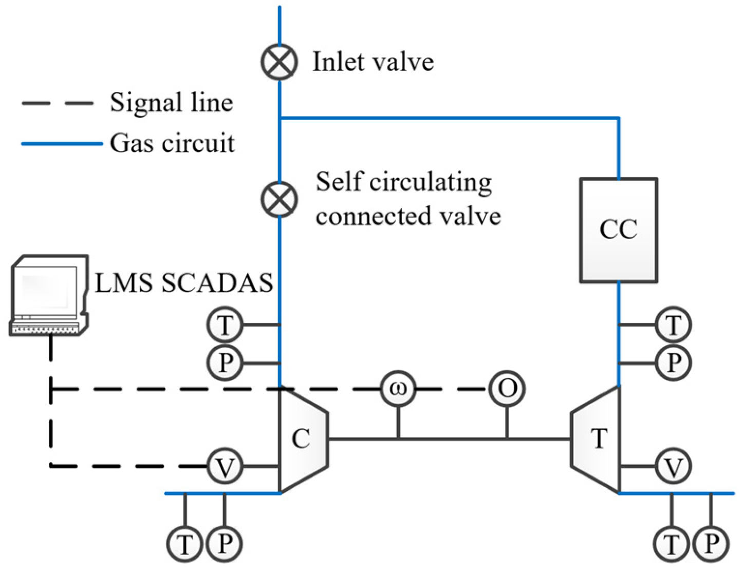
2.1. Turbocharger Bench Test

To obtain actual turbocharger measurement data for simulation model calibration, a kind of turbocharger was tested on the experiment bench under normal, dynamic imbalance and bearing wear circumstances. Temperature and pressure before and after the turbine and compressor inlet/outlet, turbocharger speed, vibration acceleration of the turbocharger base and shaft center orbit were all measured throughout the test.
Figure 1 is a schematic diagram of the test system, in which T, P and ω represent the temperature, pressure and speed sensors. V and O represent vibration and shaft centre orbit sensors. The test stand mainly consists of a turbocharger, a combustion chamber and a gas valve. The injector jets fuel into the combustion chamber for combustion. The high temperature gas enters the turbine to do work to drive the rotor shaft rotation. The coaxial compressor compresses the air. When the self-circulation valve opens, the pressurized air then enters the combustion chamber to form a self-circulation.
During the test, the temperature and pressure of the turbine and compressor intakes and outlets, the speed of the turbocharger, the vibration acceleration of the turbocharger base and the orbit of the shaft center were all measured. The Siemens LMS SCADAS Mobile system recorded the vibration, orbit of the shaft center and speed signals. The speed, temperature and pressure signals were also collected by the test bench’s measuring and control platform. The principal test instruments and equipment used in the test are shown in Table 1.
The turbocharger was put through four tests: severe dynamic imbalance, severe dynamic imbalance with bearing wear, minor dynamic imbalance and normal condition. First, a severe dynamic imbalance failure test was performed; second, a dual failure test of severe dynamic imbalance plus bearing wear was performed by replacing the faulty bearing; third, the normal bearing was replaced and the rotor dynamic imbalance was reduced on the dynamic balancing machine for a slight dynamic imbalance failure test; and finally, the dynamic imbalance of the rotor was reduced to a normal value on the dynamic balancing machine for a normal condition test. The turbocharger’s speed ranges from 35,000 r/min to 60,000 r/min, with a 2500 r/min gap. Additionally, the test program is shown in Table 2. There are two tests for dynamic unbalance. Its condition characterization parameters are the dynamic unbalance of the rotor, and the unit is mg·mm. The condition characterization parameters were 10 and 7.6, respectively. In the dynamic unbalance plus bearing wear condition, there is one test. In the normal status, there is one test. Similarly, their state characteristics parameters and units can be found in the table.

2.2. Turbocharger Model

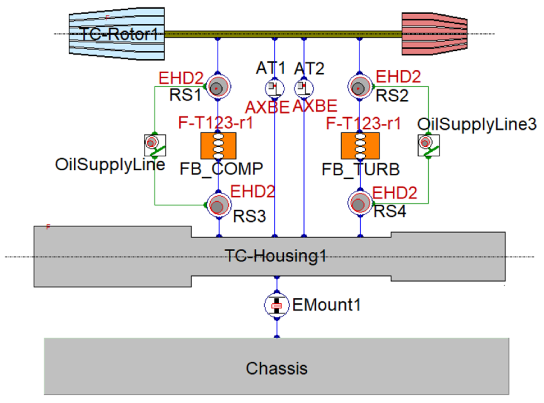
2.2.1. Whole Machine Model

The primary structure of the turbocharger includes the housing, rotor and floating ring bearing, which are the three main structures influencing the turbocharger’s multi-body dynamics computation. The software is used to build the general framework of the turbocharger dynamics model, and the established model is illustrated in Figure 2. In the figure, TC-Rotor represents the turbocharger rotor with turbine and compressor blades, RS represents the bearing connection, TS-Housing represents the turbocharger housing, chassis represents the chassis and EMount represents the mounts. The global parameters of the computational model are set by Crank Train Global. Then, the connection types of the model are defined. Additionally, the file geometry, degrees of freedom, stiffness and mass of the entire part obtained by modal reduction are introduced into the AVL Excite software platform through the software interface. After defining the loading nodes, the multi-body dynamics model is completed.
The plain bearings involved in the model are radial plain bearings. Therefore, in addition to the bearing load state, the lubrication state of the bearing should also be considered. The calculation takes into account the elastic deformation of the bearing structure, bearing clearance, journal misalignment, oil groove oil hole and oil supply conditions. A complex elastomeric hydrodynamic lubricated bearing type is selected as the connecting unit. According to this bearing type, single-point to multi-point coupling form is used to simulate the wedge effect and squeeze effect.

2.2.2. Input of Model Parameters

After the establishment of the turbocharger model, the parameters of each component are entered, and the turbocharger rotor, bearing, turbocharger housing and chassis are set. The focus of modelling is on the rotor, housing and bearing parameters. The needed parameters for elastohydrodynamic (EHD) bearing calculation include lubricant quality, bearing geometry parameters and so on. The precise non-confidential data are presented in Table 3. The rotor is modelled using the rotor shaft diameter, compressor impeller eccentricity and turbine impeller eccentricity. The floating ring bearing is modelled using the inner diameter of the floating ring, the outside diameter of the floating ring and the size of the floating ring. The rest of the parameters are used to build the oil film model.
The turbocharger speed and step settings are shown in Figure 3. Additionally, the rotor speed is applied to the kinetic model during the computation, i.e., the model boundary settings. The real turbocharger running speed is in the 35,000~60,000 r/min range, and the calculation interval is 2500 r/min, which matches the test speed.

2.2.3. Finite Element Division and Modal Reduction of Turbocharger Substructure

The turbocharger housing, rotor and floating ring bearing are all considered elastomers. Additionally, finite element modelling method is used. The turbocharger’s major structure is cleaned up; threaded holes, chamfers and other structures that are not appropriate for meshing are eliminated; and the second-order tetrahedron is utilized for finite element division of the turbocharger’s main structure.
The hypermesh software was used to divide the grid. A grid-independent test is performed. The model is divided into tetrahedral meshes with the number of (40, 60, 80, 100, 120, 140) × 104. As the number of meshes increases, the model calculation results tend to be stable. When the number of meshes increases to 80 × 104, the vibration variation rate is less than 1%. Therefore, the number of grids is set to about 80 × 104, which can satisfy the calculation accuracy requirement.
After dividing the grid, the turbocharger shell and rotor are pre-processed, and the connection surface between the shell and chassis is constrained to simulate the operating condition of the turbocharger during the actual test. The three-way degrees of freedom at the contact location between the floating ring bearing and the rotor must be preserved in the EHD calculation, with 7 nodes at the journal centerline and 70 nodes in the circumferential direction. Following the aforementioned parameters, the modal reduction of each substructure is performed. Additionally, the stiffness and mass matrices are created, which may be utilized in subsequent dynamics computations.

2.2.4. EHD Bearing Modelling

A crucial component of the turbocharger model is the floating ring-bearing multi-body dynamics model. In comparison to the rigid hydraulic lubrication bearing model, the EHD bearing model considers the lubricant’s extra viscous pressure effect, the roughness of the contact surface and the elastic deformation. Nodes for modal reduction are defined on the surfaces of the rotor journal, floating ring bearings and shaft shingles. The corresponding connection relationships are established after the nodes are reduced. The inner bearing of the floating ring in the model employs a single-point to multi-point connection to link the journal to the inner surface of the bearing.
The actual turbocharger has three oil holes on the circle of the floating ring bearing. More realistic lubricating oil pressure boundary conditions and the actual operating state of the floating ring bearing were taken into account. Three oil holes with a diameter of 3 mm around the perimeter of the floating ring bearing were uniformly added. The interaction of oil pressure between the inner and outer oil film is thoroughly considered. Meanwhile, the centrifugal force of the oil film, the friction created by the bearing motion, and the friction generated by the bearing motion are all extensively considered in the model.

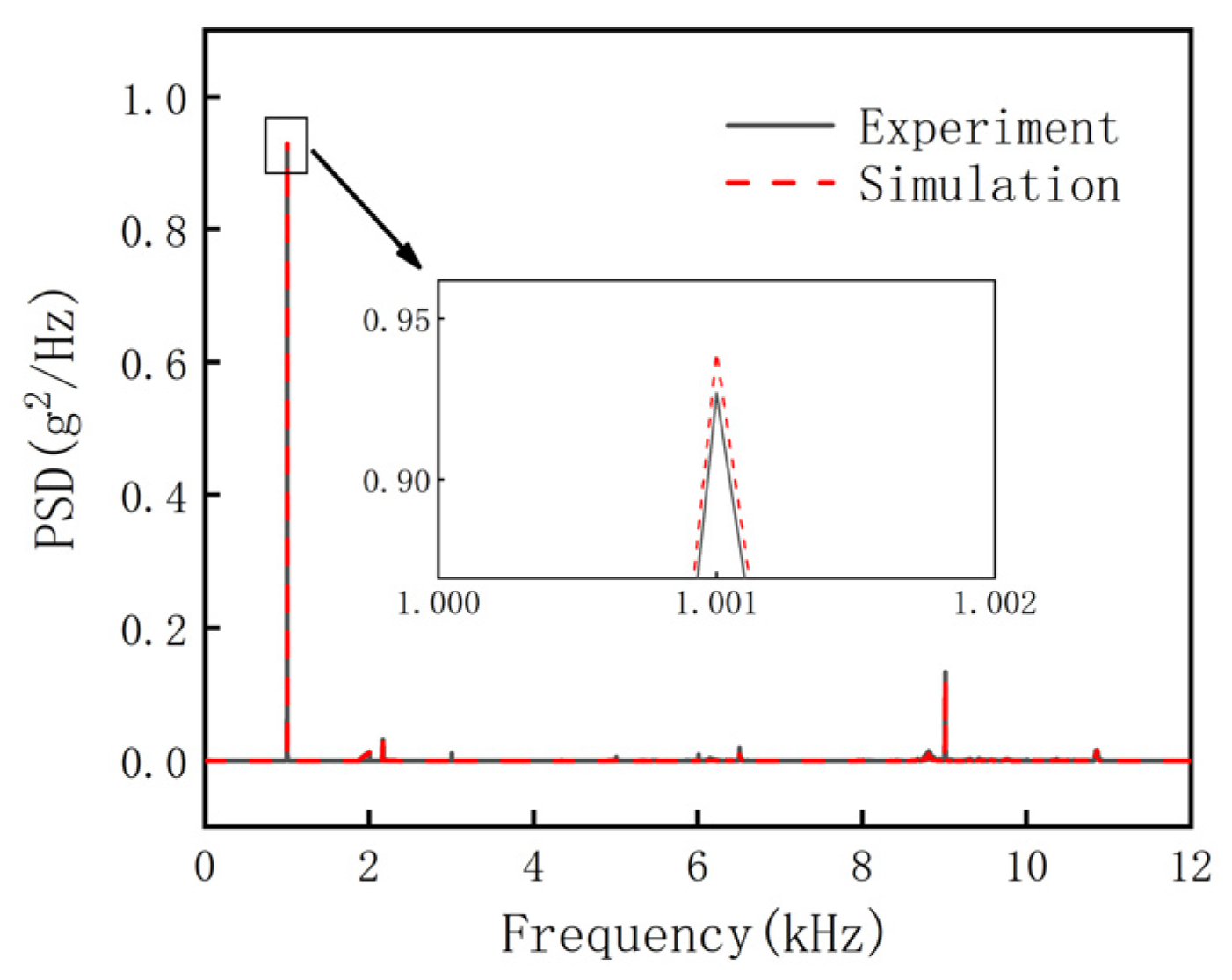
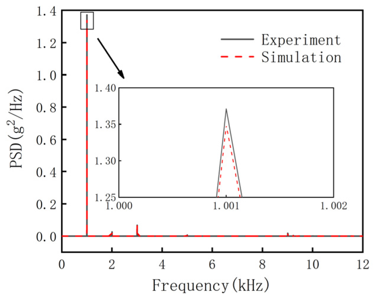
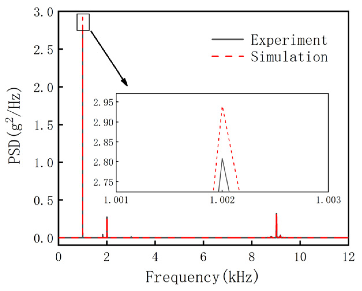
2.3. Model Validation

The accuracy of the proposed model was verified by the measured data of the turbocharger at 35,000 r/min, 37,500 r/min, 40,000 r/min … 60,000 r/min operating conditions. The frequency spectrum of the vibration signal, the shaft centre orbit, and the vibration power spectrum density (PSD) waterfall plot were calibrated. At 60,000 r/min operating conditions, the comparison between the simulation PSD of the vibration signal and the test PSD is shown in Figure 4. It shows that in the low frequency region of 0~4 kHz, the medium frequency region of 4~8 kHz and the high frequency region of 8~12 kHz, the calculated vibration curve of the turbocharger base and the test curve maintain a high consistency in trend and value. The maximum error of the simulation result is 4.9%. The modal reduction process simplifies the turbocharger appropriately, so a certain amount of error is introduced. However, the error is within 5%, which is acceptable. The calculated model and the test data of the turbocharger are in good agreement.
To further validate the correctness of the model fault simulation, the model was calibrated using dynamic unbalance fault and double fault test data. A double fault is dynamic unbalance superimposed on bearing wear fault. Figure 5 and Figure 6 show a comparison of the PSD of the vibration signal at 60,000 r/min operating conditions. The simulation result curves and the test curves match well in the low frequency zone of 0~4 kHz, the medium frequency region of 4~8 kHz, and the high frequency region of 8~12 kHz, with maximum errors of 4.5% and 4.7%, respectively. The mistake has the same origin as in the normal state simulation. The margin of error is lower than 5%, which is acceptable. Therefore, the proposed model can meet the accuracy requirements of the subsequent turbocharger dynamics fault simulation.
Comparing Figure 5 with Figure 4, the amplitude rises at 1k Hz. At 60,000 r/min operating conditions, the 1× frequency is 1k Hz. Because when the turbocharger changes from the normal state to dynamic unbalance, the rotor rotates once, which itself will produce a shock. Additionally, its vibration response characteristics will be reflected in the 1× frequency, resulting in the 1× frequency amplitude rise. The impeller has 9 main blades and 9 slave blades. At the same time, the rotor rotates once, then the impeller blade air pass occurs 9 times. It produces air pass vibration 9 times. This is the so-called blade pass frequency. Its vibration response characteristics are reflected in the 9× frequency. When the turbocharger changes from normal condition to bearing wear, its 1×, 2× and 9× frequency amplitudes change.

3. Fault Simulation and Its Data Analysis

After establishing the marine turbocharger dynamics model, the fault simulation is conducted and the fault data are examined.

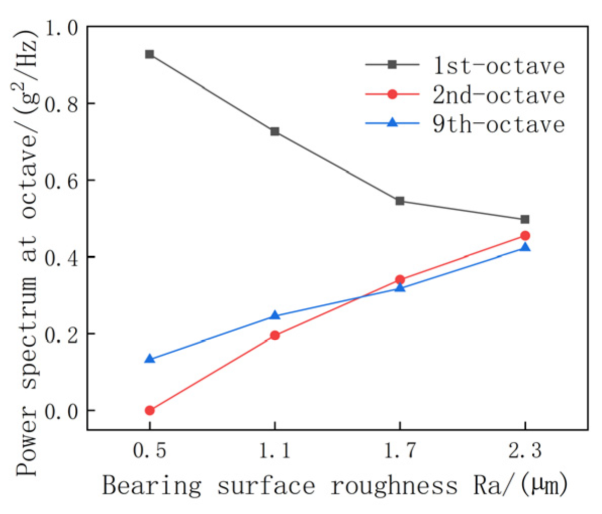
3.1. Bearing Wear Simulation

Bearing failure is a common cause of turbocharger failure. External influences cause the turbocharger bearings to wear over long periods of operation. Additionally, the wear directly alters the roughness of the inner surface of the bearings. The condition of the oil film between the bearings changes. The stability and safety of rotor operation are impacted by the bearing wear. The bearing is altered due to long-term corrosion and scouring by high-pressure oil. It increases surface roughness. Serious bearing wear leads to the oil film being unable to be established. It also causes dry friction and welding of the journal and bearing. The normal roughness of the turbocharger is 0.5 µm. The working condition of the turbocharger was simulated at 1.1, 1.7 and 2.3 bearing roughness.
Table 4 shows the variation of turbocharger parameters under normal and fault conditions. The data in it are obtained by selecting the data from 10 cycles of turbocharger operation for analysis. It can be seen that as the bearing wear increases, the time domain signal acceleration peak, peak-to-peak and root-mean-square values increase. This is because, as the bearing surface roughness increases, poor lubrication makes the rotor rotation deteriorate. It increases rotor vibration, which is transmitted to the turbocharger housing and base through the oil film, bearing and bearing seat. Then, the peak, peak-to-peak and root mean square values of vibration acceleration on the base increase. As the bearing roughness gradually becomes larger from the normal amount, the energy ratio in the 2–4 k band and the energy ratio in the 8–10 k band rise.
Figure 7 shows the variation of power spectrum amplitude of 1×, 2× and 9× octaves with the roughness of the bearing surface. The 1× octave power spectrum amplitude decreases with the increase in bearing surface roughness. Meanwhile, the 2× and 9× octave power spectra amplitude increases with the increase in roughness.

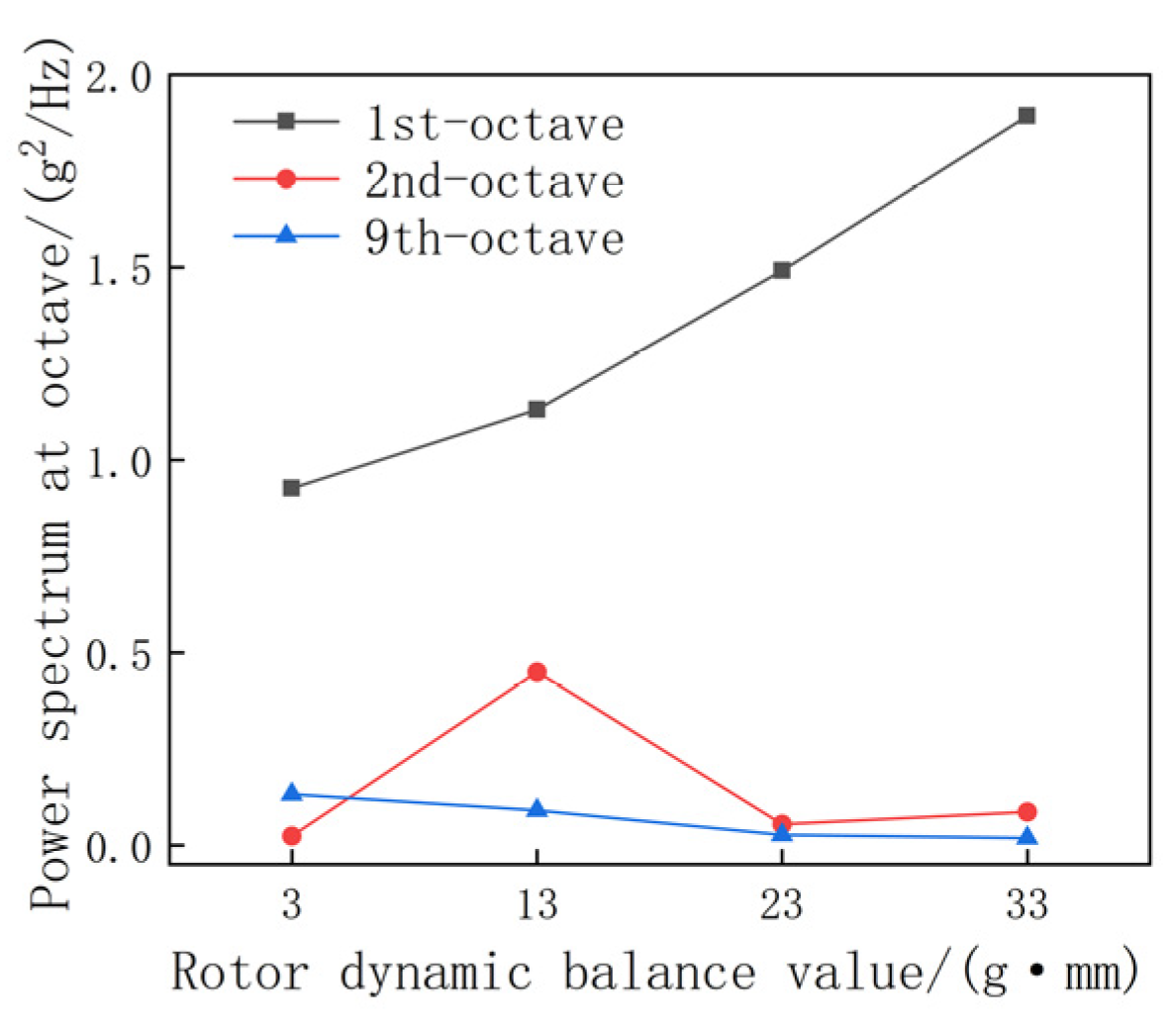
3.2. Dynamic Unbalance Simulation

Dynamic imbalance is a common turbocharger failure. Turbocharger impeller rotor and turbocharger shell scraping, rotor blade oil accumulation or foreign object strike will cause an increase in rotor dynamic imbalance or vibration amplitude. If the rotor dynamic imbalance is severe, its circle rotation of the low circumferential vortex will be more violent. It may lead to the oil film instability, journal and bearing weld. In severe cases, this can cause impeller damage, resulting in serious safety accidents. The turbocharger’s condition was simulated for the rotor dynamic balancing values of 3, 13, 23 and 33 g·mm.
Table 5 shows the variation of turbocharger parameters under normal and dynamic unbalance conditions. It can be seen that as the degree of dynamic unbalance increases, the peak acceleration, peak-to-peak and root mean square values of the time domain signal rise significantly. Because when the turbocharger rotor is unbalanced, the rotor rotates once, which itself will produce a shock. Additionally, its 1× frequency vibration will increase significantly, resulting in the rise of the above time domain signal. When the rotor dynamic imbalance becomes larger, the energy ratio rises in the 0–2 k band and falls in the 8–10 k band.
Figure 8 shows the variation of the power spectrum amplitude of the 1×, 2× and 9× vibration signals with the rotor dynamic unbalance. The amplitude of the 1× vibration signal power spectrum grows as the rotor dynamic imbalance increases. Additionally, the 9× vibration signal power spectrum amplitude decreases with the increase in the rotor dynamic unbalance.

4. Turbocharger Fault Feature Extraction

The author’s earlier proposed multi-objective matched synchrosqueezing chirplet transform (MOMSSCT) is a time–frequency analysis approach specialized in dealing with strong time-varying signals. It can better handle vibration signals from rotating machinery such as turbochargers. The approach is based on the linear chirplet transform (LCT). The steps of the LCT are to add a demodulation factor to the Fourier transform. A set of different rotation angles and demodulation rates is given. Then, the appropriate demodulation parameters are selected for calculation. The specific calculation steps of the LCT are as follows:
G ( c , t , ω ) = + s ( u ) g ( u t ) e i ω ( u t ) e ic ( u t ) 2 / 2 d u
c = tan ( β ) F s 2 T s
β = π 2 + π N c + 1 , π 2 + 2 π N c + 1 , , π 2 + N c π N c + 1
Nc is the number of demodulation rates. The sampling time  T s  and sampling frequency  F s  form a time–frequency plane. The relationship between the rotation angle β and the demodulation rate c in the time–frequency plane is given in (2). The original LCT method is based on the principle of maximum time–frequency coefficient. Then, the appropriate demodulation parameters is selected. However, its noise immunity is poor. Redundant LCT results are generated when the noise amplitude in the signal is larger than the amplitude of the component signal.
With four values of the Rayleigh entropy (RE), signal-to-noise ratio (SNR), root mean square error (RMSE) and peak signal-to-noise ratio (PSNR) as the target parameters, we suggest a MOMSSCT. The closer the demodulation rate and the modulation rate of the signal components are to one another and the smaller the Rayleigh entropy, the greater the time–frequency aggregation effect is. Rayleigh entropy is used to quantitatively evaluate the closeness of the demodulation rate of the windowed signal to the transform parameters. Additionally, the signal’s anti-noise effect is assessed using the SNR, RMSE and PSNR. The higher the signal-to-noise ratio is, the better noise immunity becomes. The four target parameters are calculated as follows:
R E = 1 2 log 2 | G ( t , w ) | ξ d w d t / | G ( t , w ) | d w d t
S N R = 10 log 10 i = 1 m x ( i ) 2 / i = 1 m ( s ( i ) x ( i ) ) 2
R M S E = 1 m i = 1 m ( s ( i ) x ( i ) ) 2
P S N R = 10 log 10 max x ( i ) 2 / 1 m × i = 1 m ( s ( i ) x ( i ) ) 2
where s is the time domain signal. x is the effective signal. Additionally, m is the number of sampling points. After the above analysis, the optimal demodulation rate  c ^  can be obtained as:
c ^ ( t , ω ) = arg min c R E + S N R + P S N R R M S E
Finally, the time–frequency transformation equation can be expressed as:
G c ^ ( t , ω ) = G ( c ^ , t , ω ) = k = 1 K A k ( t ) e i φ k ( t ) 2 σ π 1 i σ φ k ( t ) c ^ e σ ω φ k ( t ) 2 2 1 i σ φ k ( t ) c ^
where  A k ( t )  is the amplitude of the kth component of the signal.  φ k ( t )  is the instantaneous phase of the kth component of the signal.
The bandwidth  Δ ω  of the transform is calculated by the following equation.
Δ ω 2 = 1 2 π + ω 2 G c ^ ( t , ω ) 2 d ω = 1 2 π k = 1 K A k 2 ( t ) 2 π 1 + φ k ( t ) c ^ 2 1 / 2 × + ω 2 e ω φ k ( t ) 2 1 + φ k ( t ) c ^ 2 d ω = k = 1 K A k 2 ( t ) π φ k ( t ) + 2 1 + φ k ( t ) c ^ 2
Local maximum compression of the signal is used to form a new time–frequency representation (TFR)  M G c ^ s ( t , ξ ) :
M G c ^ s ( t , ξ ) = + G c ^ ( t , ω ) δ ( ξ ω ^ ( t , ω ) ) d ω
where the instantaneous frequency estimate is calculated from Equation (12).
ω ^ ( t , ω ) = arg max ω G c ^ ( t , ω ) ,   ω [ ω Δ , ω + Δ ] , if   G c ^ ( t , ω ) 0 0 , if   G c ^ ( t , ω ) = 0
The signal reconstruction is calculated as:
s ( t ) = 1 2 π g ^ ( 0 ) + + M G c ^ s ( u , ξ ) e i ω t d u d ξ
where  g ^ ( ω )  is the Fourier transform of the window function.
MOMSSCT is performed on the turbocharger to obtain the time–frequency transformation results. Then, the 1×, 2× and 9× frequency time-domain signals of the turbocharger are reconstructed from the time–frequency transformation results. The RMS values of the turbocharger’s 1× vibration, 2× vibration, 9× vibration, rotor unbalance factor and bearing wear factor are extracted as the fault characteristic parameters. The calculation equations are as follows.
1. RMS value of rotor frequency vibration  R 1 , unit m/s2.
R 1 = 1 K k = 1 K x 1 k 2
The rotor n× frequency vibration component waveform of the vibration signal waveform is noted as xnk.
2. RMS value of rotor 2× frequency vibration  R 2 , unit m/s2.
R 2 = 1 K k = 1 K x 2 k 2
3. RMS value of rotor 9× frequency vibration  R 9 , unit m/s2.
R 9 = 1 K k = 1 K x 9 k 2
4. Rotor unbalance factor  α 1 , unit m.
α 1 = R 1 / f N 2
f N  is the rotor 1× frequency and unit Hz.
5. Bearing wear factor  α 2 , dimensionless.
α 2 = R 2 / 2 f N 2

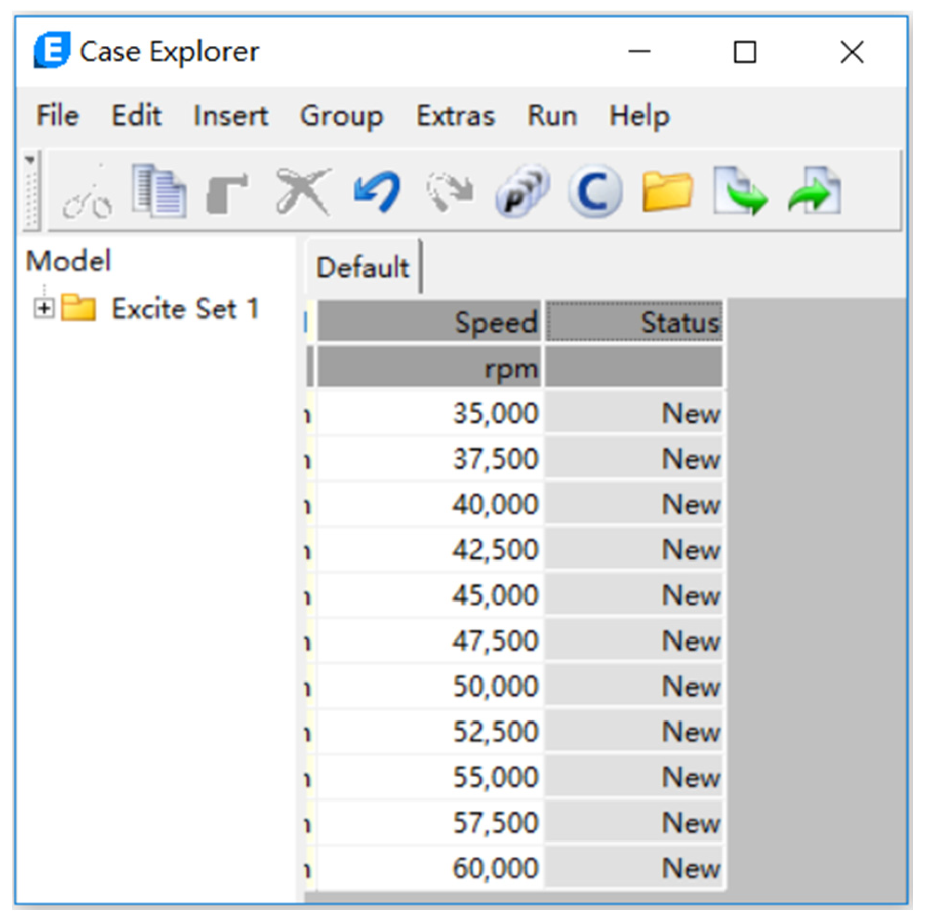
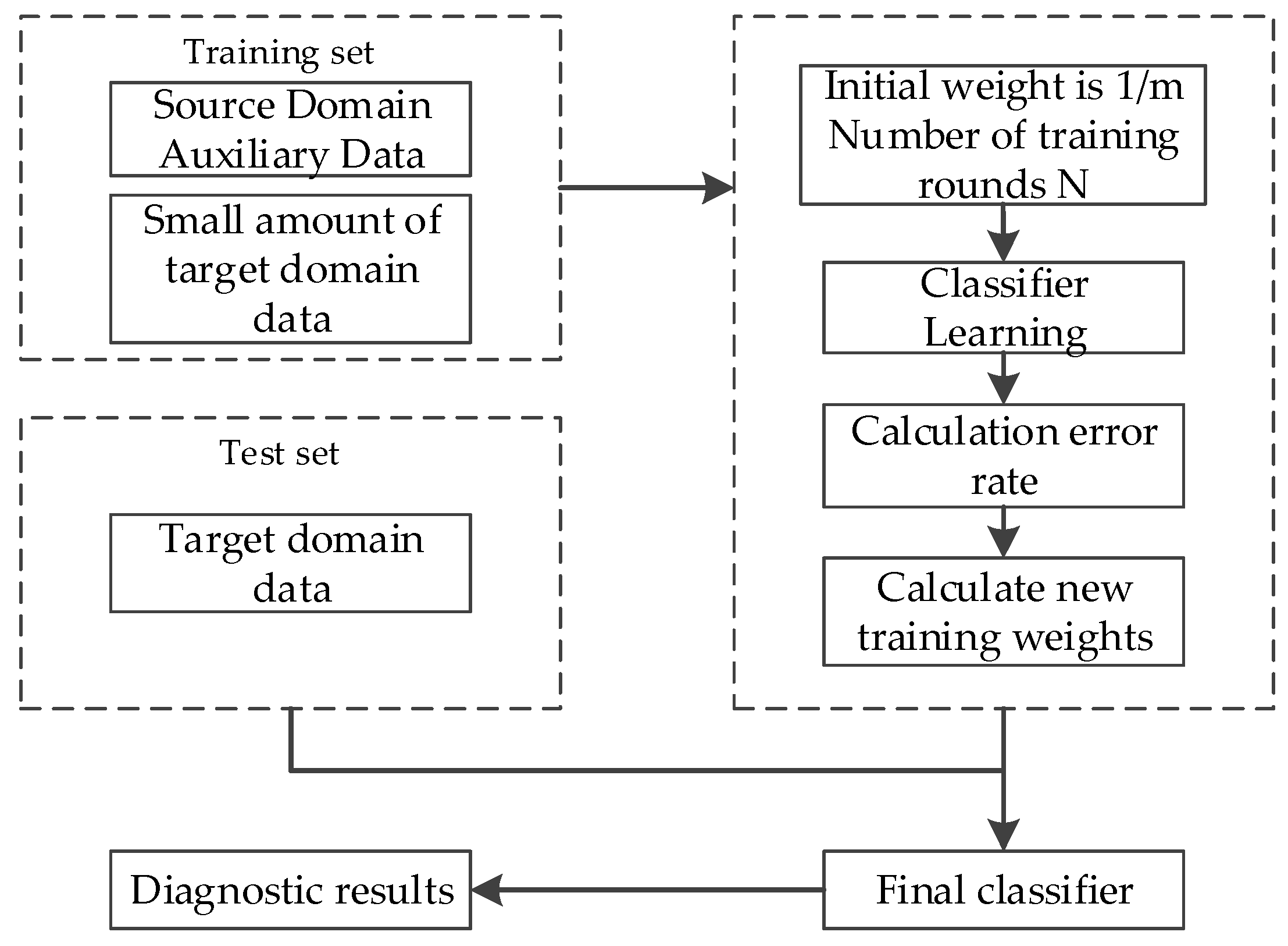
5. Transfer Learning Based Turbocharger Fault Diagnosis Method

5.1. TrAdaBoost Algorithm

Transfer learning is the transfer of knowledge between different but similar data and domains. It consists of two elements: “domain” and “task”. The domain consists of feature space and edge probability distribution. TrAdaBoost is a transfer learning algorithm based on the idea of instantiation and boosting, which is suitable for solving small sample and poor data problems. The computational flow of TrAdaBoost is shown in Figure 9, whose training set consists of a small amount of target domain data and a large amount of auxiliary data. The initial weight of the training set data is set to 1/m and the number of training rounds is N. The output prediction of the classifier is calculated based on the weights and the test set. The error rate is calculated based on the prediction results. New weights are calculated based on the error rate. The weight of misclassified target domain data is increased in the calculation process. The similarity between the auxiliary data and the target data is judged according to the classification results of each iteration. According to the result, the weights of similar data in the auxiliary data are increased and the weights of dissimilar data are decreased to obtain the final classifier. A fault diagnosis model using fewer target data was constructed [31,32].
The Xa is defined as the auxiliary domain sample space and Xb as the source domain sample space, which together form the joint training set X. The test set is defined as S.
The goal of TrAdaBoost is to build a classification model by a source domain dataset with a small amount of data and an auxiliary training set with a large amount of data. In this model, the test dataset minimizes the error.
The steps of the TrAdaBoost algorithm are as follows [31]: (1) Set the number of iterations to N, create the initial weight vector  w 1  and assign values as shown in Equations (19) and (20). (2) Calculate the distribution  p t , as shown in Equation (21). A base machine learning algorithm is given  p t , the training set X and the test set S. It computes the output prediction ht. Meanwhile, the error  ε t  of the prediction is shown in Equation (22). In the calculation process, make sure that  ε t 0.5 , if greater than 0.5,  ε t = 0.5  is taken. (3) Weight calculation factor γ and learning machine weights  β t  are calculated by Equations (23) and (24). Updating the training weights is shown in Equation (25). Additionally, repeat steps (2) and (3). (4) After reaching the maximum number of iterations N, the final hypothesis  h f ( x )  is output as shown in Equation (26).
w 1 = ( w 1 1 , , w m + n 1 )
w i 1 = 1 n , i = 1 , 2 , 3 n 1 m , i = n + 1 , n + 2 , n + m
p t = w t i = 1 n + m w i t   ( t = 1 ,   2 ,   ,   N )
ε t = i = n + 1 n + m w i t h t ( x i ) c ( x i ) i = n + 1 n + m w i t
γ = 1 / ( 1 + 2 ln n / N )
β t = ε t 1 ε t
w i t + 1 = w i t γ h t ( x i ) c ( x i ) , i = 1 , 2 , 3 n w i t β t h t ( x i ) c ( x i ) , i = n + 1 , n + 2 , n + m
h f ( x ) = 1 , t = N 2 N β t h t ( x ) t = N 2 N β t 1 2 0 , o t h e r
where N is the maximum number of iterations. n is the number of samples in the auxiliary training set. m is the number of samples in the source domain training set.  c ( x i )  is the true label value of the data. xi (i = 1, 2, …, n) is the sample in Xa. xi (i = n + 1, n + 2, …, n + m) is the sample in Xb. Algorithm 1 is the implementation code of TrAdaBoost.
Algorithm 1 TrAdaBoost
Step 1: Initialization
Input N, X, S and  w 1  by Equation (20).
Step 2: Update weight
for t = 1:N
Calculate  p t , ht ε t  by Equation (21) and (22).
If  ε t > 0.5 , take  ε t = 0.5 .
Use the value of  ε t  and ht to calculate  γ β t  and  w i t + 1  by Equations (23)~(25).
end for
Step 3: Output the hypothesis
Calculate  h f ( x )  by Equation (26).

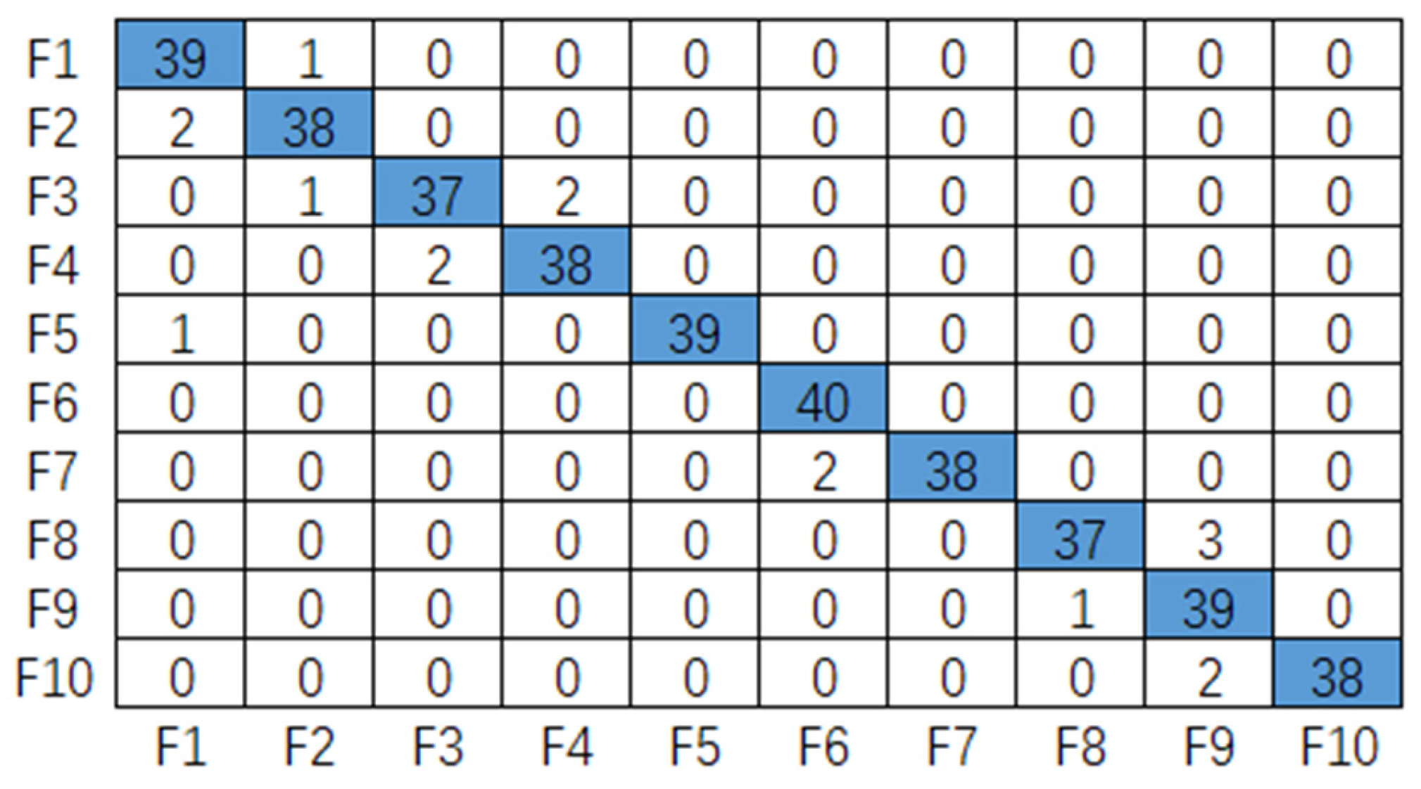
5.2. Model Diagnostic Effect

To verify the effectiveness of the diagnosis method, the turbocharger failure data was simulated. Three kinds of fault data of turbochargers under conditions of 35,000, 40,000, 50,000 and 60,000 r/min were simulated. Simulation data are used as source domain auxiliary data. The measured fault characteristic data of the turbocharger is taken as target domain data. Each fault is divided into three different degrees of failure. The data set was also divided into a training set and a test set according to a certain ratio, as shown in Table 6 and Table 7. The total number of sample data for simulation is 2040. The number of source domain auxiliary training samples is 1600 (4 loads, 10 fault states, 40 samples for each state). The number of target domain data in the training set is 20 and 40, respectively. Additionally, the number of target domain samples is 400 (4 loads, 10 fault states, 10 samples for each state).
As shown in Table 7, the training set contains a small amount of target domain data, whose numbers are 20 and 40, respectively. The test set contains a large amount of target domain data with untagged state labels, the number of which is 400. The data in the test set are the actual measured turbocharger data on the test stand. Additionally, the data in the training set are the data simulated using the turbocharger model plus very few actual measured data. If the diagnosis success rate is high, it indicates that the diagnosis model is able to achieve the knowledge transfer between the turbocharger simulation model and the real machine.
After the diagnostic model is trained, it is validated. The 400 sample data in the test set were diagnosed by the diagnostic model. The labels of normal, slight unbalance, medium unbalance, severe unbalance, etc., were defined as F1~F10, which also included the labels of two combinations of faults. The confusion matrix results are shown in Figure 10 for when the number of data in the target domain of the training set was 40.
The confusion matrix can analyze the diagnostic effect of the fault diagnosis model more intuitively and conveniently. The total of each row represents the real number of data in a certain category, and the total of each column indicates the number of data predicted as that category. Take the third row as an example; it means that the actual number of F3 labels is 40. Additionally, the fault diagnosis model predicts 37 correctly, among which one is predicted as F2 and two are predicted as F4. The larger the number on the blue diagonal, the better the diagnosis effect.
As can be seen from Figure 10, the algorithm can better distinguish between normal and fault states. However, for the dynamic unbalance slight and moderate faults, the fault diagnosis model will occur a misjudgment phenomenon because their fault characteristic parameters are more similar. Similarly, a similar situation occurs for normal and slight faults, and moderate and severe faults. For severe faults and normal states, the characteristic parameters are more different and there are basically no miscalculation occurs.
Table 8 shows the accuracy of the algorithm with different numbers of target samples in the training set. The accuracy of the algorithm increases when the number of target samples in the training set increases. The accuracy of the TrAdaBoost algorithm reaches more than 85% in both cases. The algorithm changes the weights of each target sample in the training set through the training of source domain auxiliary data. It enables the fault diagnosis model to better diagnose the target domain data (measured turbocharger data). It also improves the overall recognition effect of the model on the target domain data. The diagnostic accuracy indicates that the fault diagnosis model achieves the transfer of knowledge from the turbocharger simulation model to the real machine.

6. Conclusions

1. A marine turbocharger dynamics model was developed with model errors within an acceptable 5%. The failure sample set of the turbocharger was obtained by simulation. The fault simulation results were analyzed. The 1× vibration signal power spectrum amplitude decreases with the increase in bearing surface roughness, while the 2× and 9× vibration signal power spectra amplitude rises with the increase in roughness. The 1× vibration signal power spectrum amplitude rises with the increase in the rotor dynamic unbalance, and the 9× vibration signal power spectrum amplitude decreases with the increase in the rotor dynamic unbalance.
2. Faults were diagnosed using the TrAdaBoost transfer learning algorithm. The validation results of 2040 simulated fault samples show that the algorithm can distinguish normal and fault states well. However, for minor and moderate faults of dynamic imbalance, the fault diagnosis model feature individual misclassification. When the target sample number is 20, the accuracy of the diagnosis model is 87%. When the target number of samples is 40, the accuracy of the diagnosis model is 96%.
3. The model has the ability to diagnose under the condition of small sample data. It can realize the transfer of diagnosis knowledge between the turbocharger simulation model and the real machine. Further research could focus on transfer learning across more machine types of the turbocharger, or between different kinds of types.

Author Contributions

Methodology, F.D. and J.Y.; software, F.D. and Y.C.; writing—original draft preparation, F.D.; writing—review and editing, Y.C. and L.X.; supervision, J.Y. All authors have read and agreed to the published version of the manuscript.

Funding

This research received no external funding.

Institutional Review Board Statement

Not applicable.

Informed Consent Statement

Not applicable.

Data Availability Statement

Not applicable.

Conflicts of Interest

The authors declare no conflict of interest.

Nomenclature

  G Result of linear chirplet transform
  s ( u ) Time domain signal
  g ( t ) Window function
cDemodulation rate
βRotation angle
  F s Sampling rate
  T s Sampling time
NcNumber of demodulation rates
RERayleigh entropy
SNRSignal-to-noise ratio
RMSERoot mean square error
PSNRPeak signal-to-noise ratio
xEffective signal
mNumber of sampling points
  φ k ( t ) Instantaneous phase of the kth component of the signal
  A k ( t ) Amplitude of the kth component of the signal
  M G c ^ s ( t , ξ ) Result of linear MOMSSCT
δThe dirichlet function
ΔBand width
  R n RMS value of rotor n× frequency vibration
xnkThe rotor n× frequency vibration component waveform
  α 1 Rotor unbalance factor
  f N Rotor 1× frequency
  α 2 Bearing wear factor
XJoint training set
XaAuxiliary domain sample space
XbSource domain sample space
STest set
  w 1 Initial weight vector
  p t Distribution
htOutput prediction
  ε t Error
γWeight calculation factor
  β t Learning machine weights
NThe maximum number of iterations
  h f ( x ) Hypothesis
nNumber of samples
mNumber of samples in the source domain training set
  c ( x i ) True label value of the data
xi (i = 1, 2, …, n)Sample in Xa
xi (i = n + 1, …, n + m)Sample in Xb
TFRTime–frequency representation

References

  1. Varbanets, R.; Fomin, O.; Píštěk, V.; Klymenko, V.; Minchev, D.; Khrulev, A.; Zalozh, V.; Kučera, P. Acoustic Method for Estimation of Marine Low-Speed Engine Turbocharger Parameters. J. Mar. Sci. Eng. 2021, 9, 321. [Google Scholar] [CrossRef]
  2. Knežević, V.; Orović, J.; Stazić, L.; Čulin, J. Fault Tree Analysis and Failure Diagnosis of Marine Diesel Engine Turbocharger System. J. Mar. Sci. Eng. 2020, 8, 1004. [Google Scholar] [CrossRef]
  3. Mashhadi, P.S.; Nowaczyk, S.; Pashami, S. Stacked Ensemble of Recurrent Neural Networks for Predicting Turbocharger Remaining Useful Life. Appl. Sci. 2020, 10, 69. [Google Scholar] [CrossRef] [Green Version]
  4. Marelli, S.; Carraro, C.; Marmorato, G.; Zamboni, G.; Capobianco, M. Experimental analysis on the performance of a turbocharger compressor in the unstable operating region and close to the surge limit. Exp. Therm. Fluid Sci. 2014, 53, 154–160. [Google Scholar] [CrossRef]
  5. Li, C.H. Dynamics of rotor bearing systems supported by floating ring bearings. J. Tribol. 1982, 104, 469–477. [Google Scholar] [CrossRef]
  6. Peixoto, T.F.; Nordmann, R.; Cavalca, K.L. Dynamic analysis of turbochargers with thermo-hydrodynamic lubrication bearings. J. Sound Vib. 2021, 505, 116140. [Google Scholar] [CrossRef]
  7. Ntonas, K.; Aretakis, N.; Roumeliotis, I.; Pariotis, E.; Paraskevopoulos, Y.; Zannis, T. Integrated simulation framework for assessing turbocharger fault effects on diesel-engine performance and operability. J. Energy Eng. 2020, 146, 04020023. [Google Scholar] [CrossRef]
  8. Koutsovasilis, P. Automotive turbocharger rotordynamics: Interaction of thrust and radial bearings in shaft motion simulation. J. Sound Vib. 2019, 455, 413–429. [Google Scholar] [CrossRef]
  9. Wang, J.; Wen, H.; Qian, H.; Guo, J.; Zhu, J.; Dong, J.; Shen, H. Typical Fault Modeling and Vibration Characteristics of the Turbocharger Rotor System. Machines 2023, 11, 311. [Google Scholar] [CrossRef]
  10. Bin, G.-F.; Huang, Y.; Guo, S.-P.; Li, X.-J.; Wang, G. Investigation of induced unbalance magnitude on dynamic characteristics of high-speed turbocharger with floating ring bearings. Chin. J. Mech. Eng. 2018, 31, 88. [Google Scholar] [CrossRef] [Green Version]
  11. Barrett, J.D. Diagnosis and fault-tolerant control. IEEE Trans. Autom. Control 2012, 49, 493–494. [Google Scholar] [CrossRef]
  12. Maliuk, A.S.; Prosvirin, A.E.; Ahmad, Z.; Kim, C.H.; Kim, J.-M. Novel bearing fault diagnosis using gaussian mixture model-based fault band selection. Sensors 2021, 21, 6579. [Google Scholar] [CrossRef] [PubMed]
  13. Fonte, M.; Reis, L.; Infante, V.; Freitas, M. Failure analysis of cylinder head studs of a four stroke marine diesel engine. Eng. Fail. Anal. 2019, 101, 298–308. [Google Scholar] [CrossRef]
  14. Dalla Vedova, M.D.; Germanà, A.; Berri, P.C.; Maggiore, P. Model-based fault detection and identification for prognostics of electromechanical actuators using genetic algorithms. Aerospace 2019, 6, 94. [Google Scholar] [CrossRef] [Green Version]
  15. Sharma, V.; Parey, A. Extraction of weak fault transients using variational mode decomposition for fault diagnosis of gearbox under varying speed. Eng. Fail. Anal. 2020, 107, 104204. [Google Scholar] [CrossRef]
  16. Ma, L.; Dong, J.; Peng, K. A novel hierarchical detection and isolation framework for quality-related multiple faults in large-scale processes. IEEE Trans. Ind. Electron. 2019, 67, 1316–1327. [Google Scholar] [CrossRef]
  17. Yin, S.; Wang, G.; Gao, H. Data-driven process monitoring based on modified orthogonal projections to latent structures. IEEE Trans. Control Syst. Technol. 2015, 24, 1480–1487. [Google Scholar] [CrossRef]
  18. Palmer, F.S.; Luber, B.; Fuchs, J.; Kern, T.; Rosenberger, M. Data-driven fault diagnosis of bogie suspension components with on-board acoustic sensors. In Proceedings of the Fifth European Conference on the Prognostics and Health Management Society, Turin, Italy, 1–3 July 2020; pp. 1–13. [Google Scholar]
  19. Li, L.; Ding, S.X.; Yang, Y.; Peng, K.; Qiu, J. A fault detection approach for nonlinear systems based on data-driven realizations of fuzzy kernel representations. IEEE Trans. Fuzzy Syst. 2017, 26, 1800–1812. [Google Scholar] [CrossRef]
  20. Said, M.; Abdellafou, K.; Taouali, O. Machine learning technique for data-driven fault detection of nonlinear processes. J. Intell. Manuf. 2020, 31, 865–884. [Google Scholar] [CrossRef]
  21. Lundgren, A.; Jung, D. Data-driven fault diagnosis analysis and open-set classification of time-series data. Control Eng. Pract. 2022, 121, 105006. [Google Scholar] [CrossRef]
  22. Stubbs, S.; Zhang, J.; Morris, J. BioProcess performance monitoring using multiway interval partial least squares. Comput. Aided Chem. Eng. 2018, 41, 243–259. [Google Scholar]
  23. He, Z.; Yang, Y.; Qiao, L.; Zhang, Y.; Han, H.; Li, H.; Liu, Z.; Yang, Y. Canonical correlation analysis and key performance indicator based fault detection scheme with application to marine diesel supercharging systems. In Proceedings of the 2019 Chinese Control Conference (CCC), Guangzhou, China, 27–30 July 2019; pp. 5156–5160. [Google Scholar]
  24. Peng, K.; Zhang, K.; You, B.; Dong, J. Quality-relevant fault monitoring based on efficient projection to latent structures with application to hot strip mill process. IET Control Theory Appl. 2015, 9, 1135–1145. [Google Scholar] [CrossRef]
  25. Liu, J.; Li, Y.; Ma, X.; Liang, W.; Liang, W.H. Fault tree analysis using bayesian optimization: A reliable and effective fault diagnosis approaches. J. Fail. Anal. Prev. 2021, 21, 619–630. [Google Scholar]
  26. Zhou, T.; Han, T.; Droguett, E.L. Towards trustworthy machine fault diagnosis: A probabilistic Bayesian deep learning framework. Reliab. Eng. Syst. Saf. 2022, 224, 108525. [Google Scholar] [CrossRef]
  27. Liu, Y.; Zhang, J.; Qin, K.; Xu, Y. Diesel engine fault diagnosis using intrinsic time-scale decomposition and multistage Adaboost relevance vector machine. Proc. Inst. Mech. Eng. Part C J. Mech. Eng. Sci. 2018, 232, 881–894. [Google Scholar] [CrossRef]
  28. Zhuang, F.; Qi, Z.; Duan, K.; Xi, D.; Zhu, Y.; Zhu, H.; Xiong, H.; He, Q. A comprehensive survey on transfer learning. Proc. IEEE 2020, 109, 43–76. [Google Scholar] [CrossRef]
  29. Jumnake, G.F.; Mahalle, P.N.; Shinde, G.R.; Thakre, P.A. Deep and Transfer Learning in Malignant Cell Classification for Colorectal Cancer. In Information Systems for Intelligent Systems: Proceedings of ISBM 2022; Springer: Singapore, 2023; pp. 319–329. [Google Scholar]
  30. Chen, W.; Qiu, Y.; Feng, Y.; Li, Y.; Kusiak, A. Diagnosis of wind turbine faults with transfer learning algorithms. Renew. Energy 2021, 163, 2053–2067. [Google Scholar] [CrossRef]
  31. Yao, Y.; Doretto, G. Boosting for transfer learning with multiple sources. In Proceedings of the 2010 IEEE Computer Society Conference on Computer Vision and Pattern Recognition, San Francisco, CA, USA, 13–18 June 2010; pp. 1855–1862. [Google Scholar]
  32. Hu, J.; Yu, Y.; Yang, J.; Jia, H. Research on the Generalisation Method of Diesel Engine Exhaust Valve Leakage Fault Diagnosis Based on Acoustic Emission. Measurement 2023, 210, 112560. [Google Scholar] [CrossRef]
Figure 1. Schematic diagram of the turbocharger test system.
Actuators 12 00146 g001
Figure 2. Turbocharger dynamics model.
Actuators 12 00146 g002
Figure 3. Turbocharger speed and step setting.
Actuators 12 00146 g003
Figure 4. Comparison between the simulated and experimental values of PSD in the normal state.
Actuators 12 00146 g004
Figure 5. Comparison between simulated and experimental values of PSD in the dynamic unbalance state.
Actuators 12 00146 g005
Figure 6. Comparison between simulated and experimental values of PSD in double fault state.
Actuators 12 00146 g006
Figure 7. Variation of each parameter at the characteristic frequency during bearing wear.
Actuators 12 00146 g007
Figure 8. Variation of each parameter at the characteristic frequency during dynamic unbalance.
Actuators 12 00146 g008
Figure 9. Calculation flow of TrAdaBoost fault diagnosis model.
Actuators 12 00146 g009
Figure 10. TrAdaBoost algorithm fault identification effect.
Actuators 12 00146 g010
Table 1. Test instruments and equipment in stand test.
Equipment NameModelRangePrecision
Turbocharger measurement and control systemNI
Vibration test systemLMS SCADAS Mobile
Acceleration sensorB&K 4534-B±700 g
orbit of the shaft centre Eddy current sensorBently330010~100 mils
Rotational speed sensorEM3309±0.5%
Temperature sensorsK index thermocouple0~1000 °C±2%
Pressure sensorsY-153BF0~1.6 MPa±0.4%
Table 2. Turbocharger failure test program table.
Turbocharger StatusCondition Characterization ParametersUnitTests
Dynamic unbalance conditionRotor dynamic unbalance and
Bearing surface roughness Ra value
mg·mm and
μm
(1) 10.0 mg·mm 0.5 μm
(2) 7.6 mg·mm 0.5 μm
Dynamic unbalance and bearing wear conditionRotor dynamic unbalance and
Bearing surface roughness Ra value
mg·mm and
μm
(1) 10.0 mg·mm 1.2 μm
Normal statusRotor dynamic unbalance and
Bearing surface roughness Ra value
mg·mm and
μm
(1) 3.1 mg·mm 0.5 μm
Table 3. Table of parameters required for model calculation.
ParameterValueUnit
The diameter of the rotor shaft12.4mm
Eccentricity of the compressor impeller2mm
Eccentricity of the turbine impeller3mm
Inner diameter of the floating ring12.4mm
Outer diameter of the floating ring17.7mm
Size of the floating ring20.2mm
The density of oil827.9kg/m3
The initial temperature of the oil film373K
The viscosity of the lubricant11.3mPa·s
Specific heat of the oil film1950J/kg·K
Thermal conductivity of the oil film0.14W/m·K
Constant α of viscosity-pressure2.2 × 10−8m2/K
Constant β of viscosity-temperature0.03K−1
Table 4. Turbocharger parameters under normal and fault conditions.
NormalMinor FailureModerate FailureSevere Failure
Time domain acceleration peak/g4.898.1611.8916.64
Peak to peak acceleration/g13.5521.4431.3942.29
Root mean square value/g2.744.145.847.57
0–2 k band energy ratio28.13%12.96%11.03%10.73%
2–4 k band energy ratio3.42%5.51%6.72%8.06%
4–6 k band energy ratio2.43%1.56%1.50%1.43%
6–8 k band energy ratio11.12%9.48%9.08%8.68%
8–10 k band energy ratio40.89%53.23%55.13%55.30%
10–12 k band energy ratio14.01%17.26%16.54%15.80%
Table 5. Turbocharger parameters under normal and dynamic unbalance conditions.
NormalMinor FailureModerate FailureSevere Failure
Time domain acceleration peak/g4.8918.7334.8348.55
Peak to peak acceleration/g13.5531.3146.3961.94
Root mean square value/g2.747.5913.9319.57
0–2 k band energy ratio28.13%31.52%35.26%72.32%
2–4 k band energy ratio3.42%3.40%0.96%6.29%
4–6 k band energy ratio2.43%2.42%2.33%2.48%
6–8 k band energy ratio11.12%11.06%16.92%1.20%
8–10 k band energy ratio40.89%37.67%22.93%9.87%
10–12 k band energy ratio14.01%13.92%21.60%7.85%
Table 6. Division of source domain auxiliary data and target domain data set.
Source Domain Auxiliary Data (Simulation)Target Domain Data (Measured)
Normal16040
dynamic unbalance480120
bearing wear480120
Dynamic unbalance combined with bearing wear480120
Table 7. Training set and test set samples.
Training SetTest Set
Data contentSource domain auxiliary dataSmall amount of target domain dataTarget domain data
Data quantity160020 or 40400
Table 8. Accuracy of the algorithm with different numbers of target samples in the training set.
Source Domain → Target DomainData1Data2
Number of target samples in the training set2040
TrAdaBoost algorithm accuracy0.870.96
Disclaimer/Publisher’s Note: The statements, opinions and data contained in all publications are solely those of the individual author(s) and contributor(s) and not of MDPI and/or the editor(s). MDPI and/or the editor(s) disclaim responsibility for any injury to people or property resulting from any ideas, methods, instructions or products referred to in the content.

