
Design and Unbiased Control of Nine-Pole Radial Magnetic Bearing


Abstract
:1. Introduction
2. Force–Current Relationship
2.1. Radial Magnetic Bearing
2.2. Force vs. Coil Currents
2.3. Unsymmetrical Bearing
3. Unsymmetrical Bearing Design
3.1. Reference Symmetric Bearing
3.2. Comparison of Unsymmetrical Designs
4. Unbiased Control Design
4.1. Force Inversion
4.2. Displacement Compensation
4.3. Unbiased Control Design
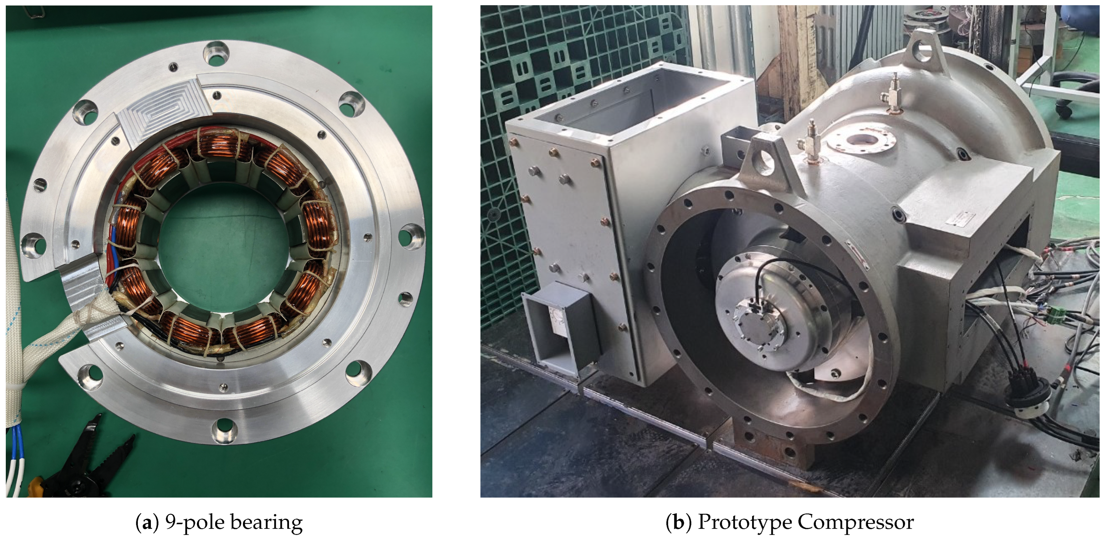
5. Experimental Setup
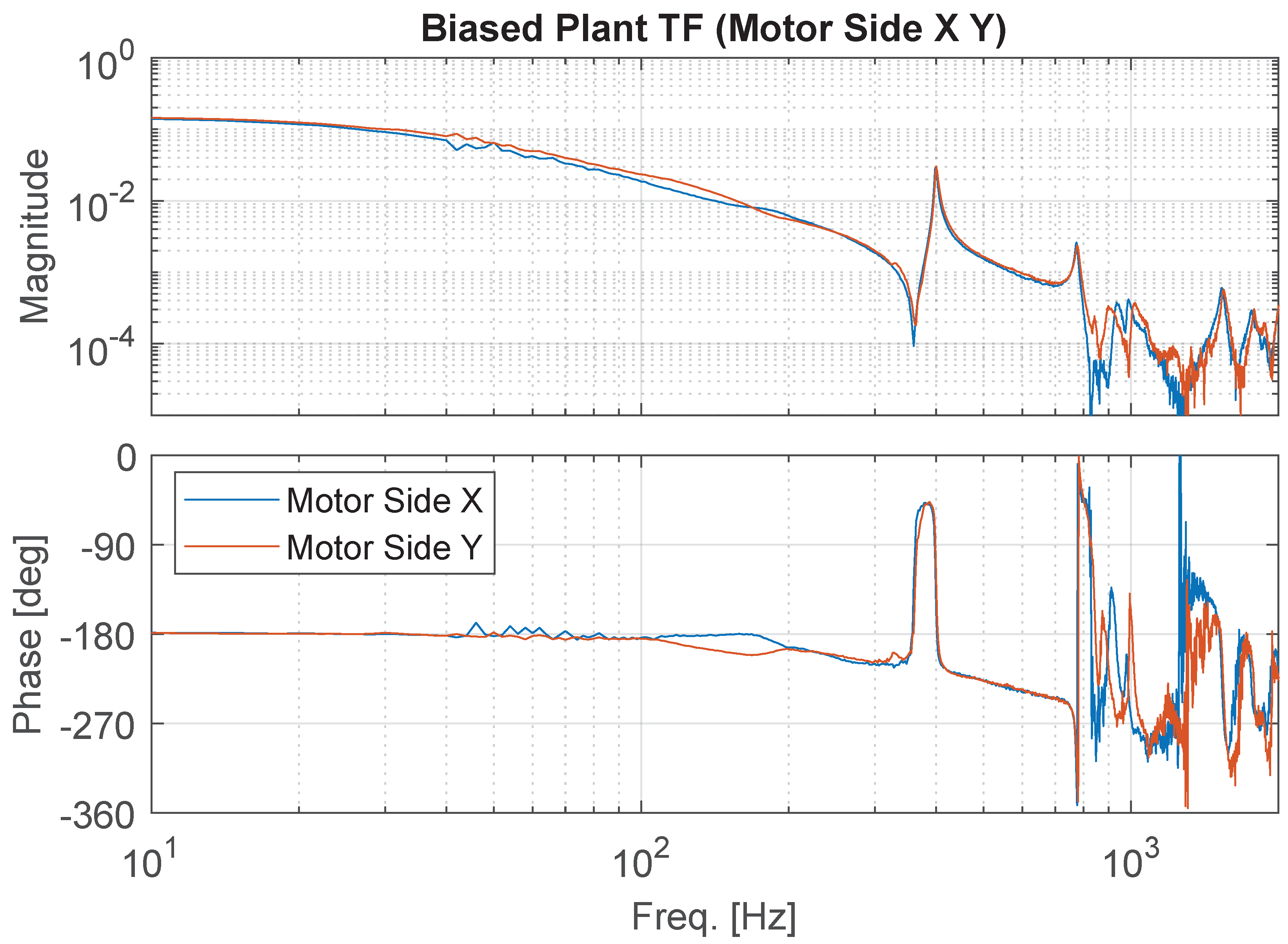
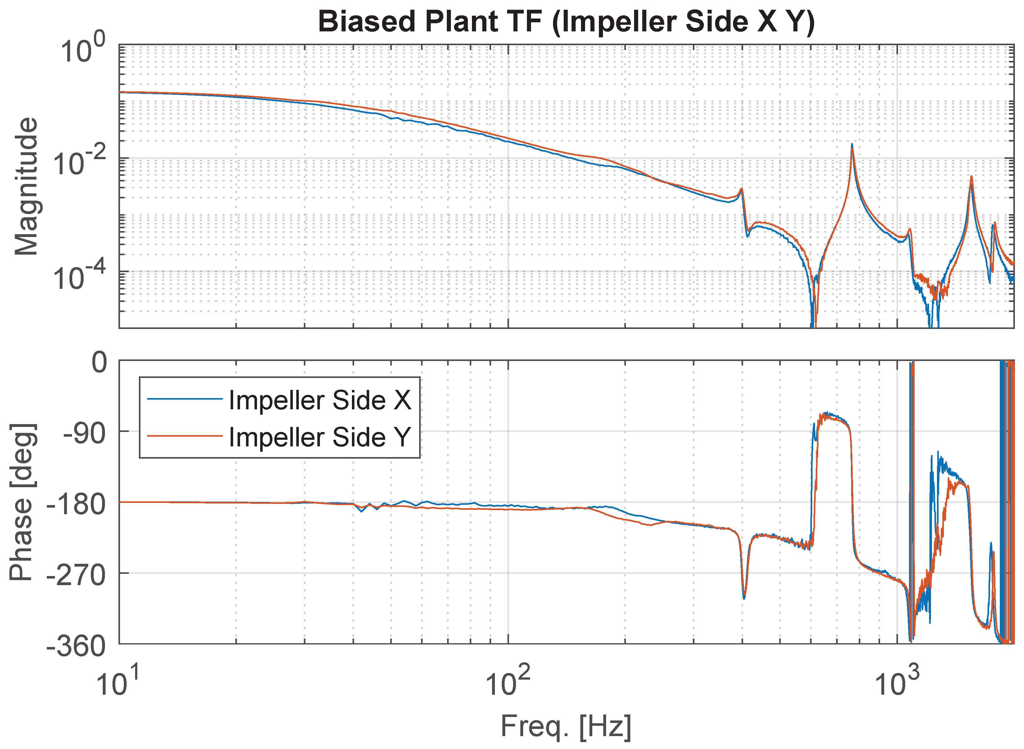
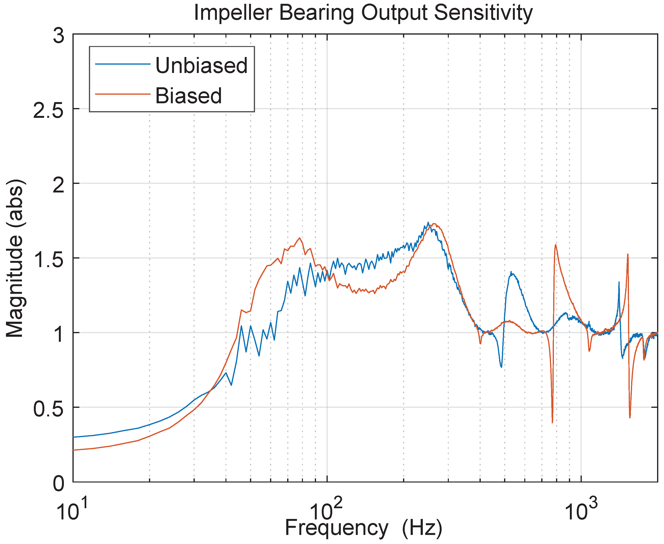
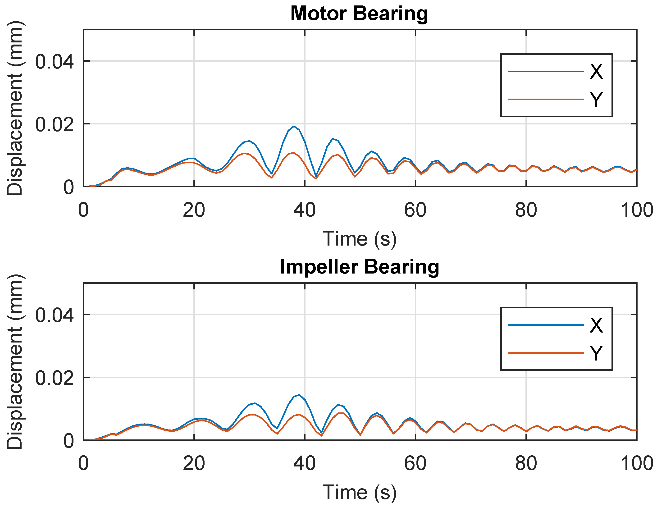
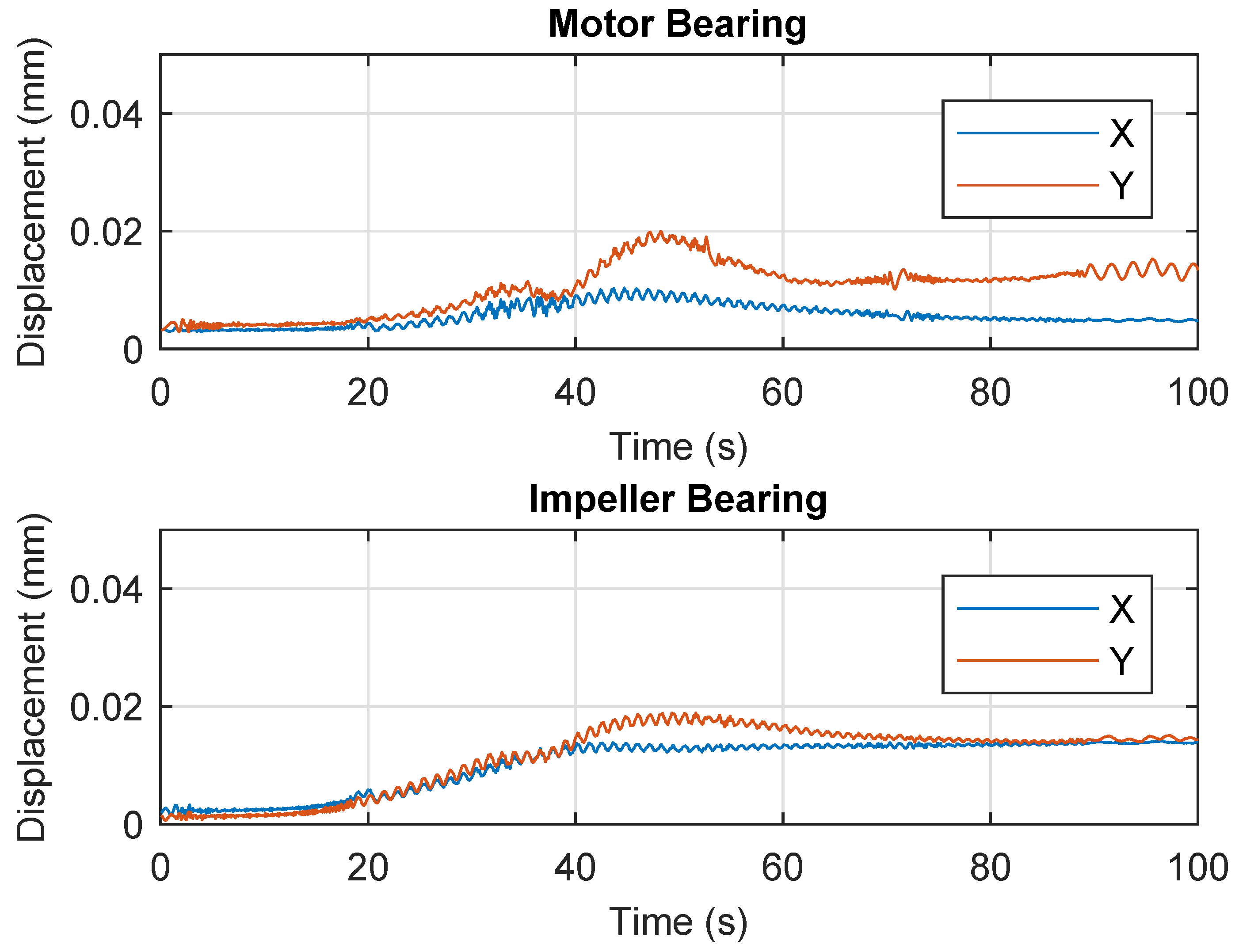
6. Results and Discussion
7. Conclusions
Author Contributions
Funding
Data Availability Statement
Conflicts of Interest
Appendix A. Reluctance and Coil Turn Matrix for 8-Pole Bearing
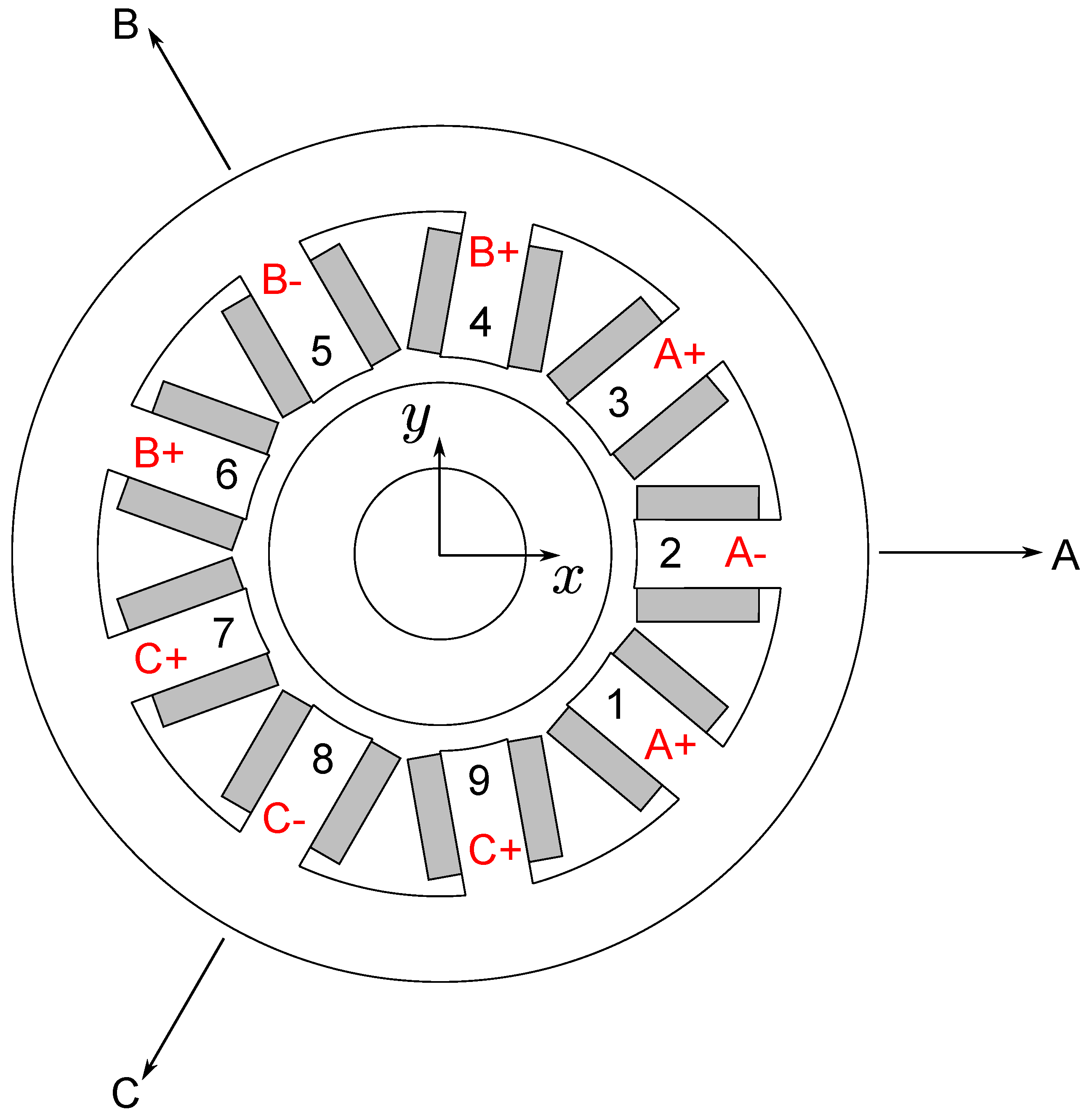
Appendix B. Coil Turn Matrix for 9-Pole Bearing
References
- Schweitzer, G.; Maslen, E.H. Magnetic Bearings; Springer: Berlin/Heidelberg, Germany, 2009. [Google Scholar]
- Trumper, D.L.; Olson, S.M.; Subrahmanyan, P.K. Linearizing Control of Magnetic Suspension Systems. IEEE Trans. Control Syst. Technol. 1997, 5, 427–438. [Google Scholar] [CrossRef]
- Li, L. Linearizing Magnetic Bearing Actuators by Constant Current Sum, Constant Voltage Sum, and Constant Flux Sum. IEEE Trans. Magn. 1999, 35, 528–535. [Google Scholar]
- Charara, A.; De Miras, J.; Caron, B. Nonlinear Control of a Magnetic Levitation System without Premagnetization. IEEE Trans. Control Syst. Technol. 1996, 4, 513–523. [Google Scholar] [CrossRef]
- Sivrioglu, S.; Nonami, K.; Saigo, M. Low Power Consumption Nonlinear Control with H∞ Compensator for a Zero-Bias Flywheel AMB System. J. Vib. Control 2004, 10, 1151–1166. [Google Scholar] [CrossRef]
- Mystkowski, A.; Pawluszewicz, E. Nonlinear Position-Flux Zero-Bias Control for AMB System with Disturbance. Appl. Comput. Electromagn. Soc. J. (ACES) 2017, 32, 650–656. [Google Scholar]
- De Queiroz, M.S.; Dawson, D.M. Nonlinear Control of Active Magnetic Bearings: A Backstepping Approach. IEEE Trans. Control Syst. Technol. 1996, 4, 545–552. [Google Scholar] [CrossRef]
- Tsiotras, P.; Wilson, B.C. Zero-and Low-Bias Control Designs for Active Magnetic Bearings. IEEE Trans. Control Syst. Technol. 2003, 11, 889–904. [Google Scholar] [CrossRef]
- Sahinkaya, M.N.; Hartavi, A.E. Variable Bias Current in Magnetic Bearings for Energy Optimization. IEEE Trans. Magn. 2007, 43, 1052–1060. [Google Scholar] [CrossRef]
- Yoo, S.y.; Noh, M.D. An Appraisal of Power-Minimizing Control Algorithms for Active Magnetic Bearings. Shock Vib. 2015, 2015, 238629. [Google Scholar] [CrossRef]
- Chen, S.L.; Hsu, C.T. Optimal Design of a Three-Pole Active Magnetic Bearing. IEEE Trans. Magn. 2002, 38, 3458–3466. [Google Scholar] [CrossRef]
- Meeker, D.C.; Maslen, E.H. Analysis and Control of a Three Pole Radial Magnetic Bearing. In Proceedings of the Tenth International Symposium on Magnetic Bearings, Martigny, Switzerland, 21–23 August 2006. [Google Scholar]
- Hemenway, N.R.; Severson, E.L. Three-Pole Magnetic Bearing Design and Actuation. IEEE Trans. Ind. Appl. 2020, 56, 6348–6359. [Google Scholar] [CrossRef]
- Zhang, H.; Zhu, H.; Wu, M. Multi-Objective Parameter Optimization-Based Design of Six-Pole Radial Hybrid Magnetic Bearing. IEEE J. Emerg. Sel. Top. Power Electron. 2021, 10, 4526–4535. [Google Scholar] [CrossRef]
- Meeker, D. A Generalized Unbiased Control Strategy for Radial Magnetic Bearings. Actuators 2017, 6, 1. [Google Scholar] [CrossRef]
- Maslen, E. Lecture Notes on Magnetic Bearings; University of Virginia: Charlottesville, VA, USA, 2000. [Google Scholar]
- Meeker, D.C. Optimal Solutions to the Inverse Problem in Quadratic Magnetic Actuators. Ph.D. Thesis, University of Virginia, Charlottesville, VA, USA, 1996. [Google Scholar]
- API617; Axial and Centrifugal Compressors and Expanders-Compressors for Petroleum, Chemical and Gas Industry Services. American Petroleum Institute: Washington, DC, USA, 2014.
- Messner, W.C.; Bedillion, M.D.; Xia, L.; Karns, D.C. Lead and Lag Compensators with Complex Poles and Zeros Design Formulas for Modeling and Loop Shaping. IEEE Control Syst. Mag. 2007, 27, 44–54. [Google Scholar]
- ISO14839-3; Mechanical Vibration—Vibration of Rotating Machinery Equipped with Active Magnetic Bearings—Part 3: Evaluation of Stability Margin. International Organization for Standardization: Geneva, Switzerland, 2006.
- ISO14839-2; Mechanical Vibration—Vibration of Rotating Machinery Equipped with Active Magnetic Bearings—Part 2: Evaluation of Vibration. International Organization for Standardization: Geneva, Switzerland, 2006.


| Parameter | Symbol | Value | Unit |
|---|---|---|---|
| Nominal gap | 0.5 | mm | |
| Number of coil turns | N | 32 | |
| Journal radius | 46.6 | mm | |
| Pole width | w | 16.6 | mm |
| Rotor shaft radius | 30 | mm | |
| Stator outer radius | 77 | mm | |
| Stator mass | 4.5 | kg | |
| Actuator gain | 141 | N/A | |
| Open-loop stiffness | −1826 | N/mm |
| Pole Count | (18) | (19) | Stator Size | Stator Mass | Rotor Size |
|---|---|---|---|---|---|
| 3 | 0.375 | 0.578 | 1.38 | 2.96 | 0.19 |
| 5 | 0.625 | 0.526 | 0.90 | 0.78 | 0.72 |
| 6 | 0.650 | 1.000 | 1.03 | 1.26 | 0.75 |
| 9 | 0.950 | 0.670 | 0.94 | 0.74 | 1.01 |
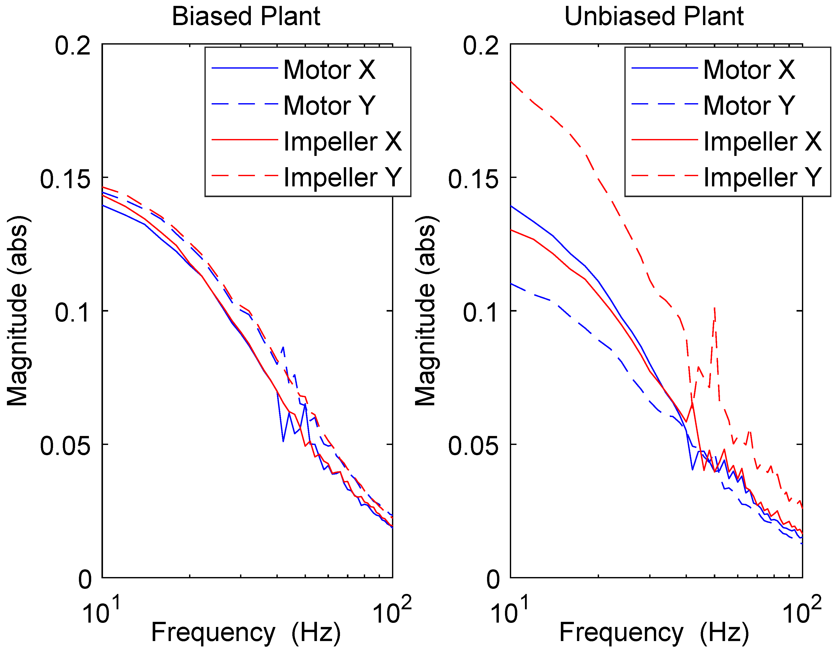
| Compressor | Bearing | X (mm/V) | Y (mm/V) | Ratio |
|---|---|---|---|---|
| Biased | Motor | 0.1395 | 0.1444 | 1.035 |
| Impeller | 0.1303 | 0.1464 | 1.123 | |
| Unbiased | Motor | 0.1395 | 0.1102 | 0.790 |
| Impeller | 0.1433 | 0.1860 | 1.298 |
Disclaimer/Publisher’s Note: The statements, opinions and data contained in all publications are solely those of the individual author(s) and contributor(s) and not of MDPI and/or the editor(s). MDPI and/or the editor(s) disclaim responsibility for any injury to people or property resulting from any ideas, methods, instructions or products referred to in the content. |
© 2023 by the authors. Licensee MDPI, Basel, Switzerland. This article is an open access article distributed under the terms and conditions of the Creative Commons Attribution (CC BY) license (https://creativecommons.org/licenses/by/4.0/).
Share and Cite
Noh, M.D.; Jeong, W. Design and Unbiased Control of Nine-Pole Radial Magnetic Bearing. Actuators 2023, 12, 458. https://doi.org/10.3390/act12120458
Noh MD, Jeong W. Design and Unbiased Control of Nine-Pole Radial Magnetic Bearing. Actuators. 2023; 12(12):458. https://doi.org/10.3390/act12120458
Chicago/Turabian StyleNoh, Myounggyu D., and Wonjin Jeong. 2023. "Design and Unbiased Control of Nine-Pole Radial Magnetic Bearing" Actuators 12, no. 12: 458. https://doi.org/10.3390/act12120458
APA StyleNoh, M. D., & Jeong, W. (2023). Design and Unbiased Control of Nine-Pole Radial Magnetic Bearing. Actuators, 12(12), 458. https://doi.org/10.3390/act12120458