Fault Feature Extraction Method of Ball Screw Based on Singular Value Decomposition, CEEMDAN and 1.5DTES

Abstract

In this article, a method is proposed to effectively extract weak fault features and accurately diagnose faults in ball screws, even in the presence of strong background noise. This method combines singular value decomposition (SVD), complete ensemble empirical mode decomposition with adaptive noise (CEEMDAN), and the 1.5-dimensional spectrum (1.5D) to process and analyze fault vibration signals. The first step involves decomposing the fault signal using the SVD algorithm. The singular values are then screened, and the part of the screen containing more noise information is extracted to complete the first denoising step. The second step involves decomposing the signal after the initial denoising process using CEEMDAN and removing some of the false components from the intrinsic mode function (IMF) components, based on the kurtosis correlation function index. The signal is then reconstructed to complete the second denoising step. Finally, the denoised signal is analyzed using Teager energy operator demodulation and 1.5D spectral analysis to extract the fault frequency and determine the location of the fault in the ball screw. This method has been compared with other denoising methods, such as wavelet packet decomposition combined with CEEMDAN or SVD combined with variational mode decomposition (VMD), and the results show that under the condition of strong background noise, the proposed method can better extract the fault frequency of ball screw.

1. Introduction

With the rise in the industrialization level and the continuous improvement of mechanical automation, ball screws are more and more widely used in industrial production. As a kind of high-precision, high-speed and high-load-transmission device, ball screws are widely used in machinery, manufacturing, aviation, rail transit, and other fields [1]. With an increase in the running time of the ball screw, various fault-related problems often occur. The fault signal of the ball screw usually presents nonlinear and non-stationary characteristics and is characterized by periodic impact characteristics. The faults generated in actual production often cause very serious consequences. The working environment is usually harsh, and the fault signal characteristics are often covered by background noise and mechanical rotation signals, which are not easy to extract. Therefore, it is necessary to develop a fault diagnosis method when working under strong background noise interference conditions [2,3].

With the development of signal-processing technology, research on the fault diagnosis of rotating machinery has achieved certain results. Shi et al. [4] proposed a bearing fault diagnosis algorithm based on wavelet multi-scale analysis and XGBoost fusion feature selection to address the problem that the rolling bearing fault signal is susceptible to the pollution of the surrounding noise environment and the difficulty of feature extraction and selection in the acquisition process. The collected sound signal is denoised by five-layer wavelet decomposition and reconstruction to filter out the doped noise signal. Wu et al. [5] proposed a method of combining wavelet denoising analysis and FastICA independent component analysis, based on negative entropy, to deal with the noisy vibration signals of rolling bearings. First, the original signal is processed by wavelet denoising, then the processed signal is combined with the original signal to form the input matrix of FastICA for FastICA denoising. However, this classical noise reduction algorithm has the problem that the wavelet basis is difficult to select, and the FastICA algorithm is generally used for bearing signal noise reduction when in actual operation. Cai et al. [6] proposed a bearing fault feature extraction method based on singular value decomposition (SVD) and variational mode decomposition (VMD) to address the problem that the impact signal contains a great deal of noise and it is difficult to extract the fault’s characteristic frequency when the bearing is weak. The results of simulation analysis and two different bearing tests show that the proposed method can effectively suppress noise and obtain signals that reflect the actual fault information. Empirical mode decomposition (EMD) is an adaptive time-frequency analysis method proposed by Huang et al. [7], but it has the defect of mode mixing. In order to solve this defect, TORRES et al. [8] proposed the CEEMDAN algorithm. Wang Zhijian et al. [9] proposed using an evaluative health index (EHI), which combines the proportional weighting method of three evaluation indexes of monotonicity, trend, and prognosis and integrates multiple sources of degradation information. Aiming to address the problem that the fault signal of wind turbine bearings is weak, difficult to extract, and difficult to identify, Liu et al. [10] proposed a fault diagnosis method for use with wind turbine bearings, based on adaptive noise complete ensemble empirical mode decomposition (CEEMDAN) and a grey wolf optimization kernel extreme learning machine (GWO-KELM). Yan et al. [11] combined the synchrosqueezed generalized S-transform of variational mode decomposition and the Teager–Kaiser energy operator and used the Teager–Kaiser energy operator to enhance the extracted attenuation gradient and effectively highlight the oil and gas area. Tang Guiji et al. [12] proposed a rolling bearing fault diagnosis method based on multivariate variational mode decomposition (MVMD) and a 1.5-dimensional spectrum. First, the 1.5-dimensional spectrum of the envelope signal is calculated, and the fault feature information extracted from the spectrum is then analyzed to diagnose the fault type. The fault diagnosis experiment of a rolling bearing proves that this method can effectively extract feature information on a weak bearing fault and achieve an accurate diagnosis of a bearing fault feature.

In order to make full use of the advantages of SVD, CEEMDAN, and the 1.5D spectrum in terms of noise reduction and feature extraction, this paper proposes combining the three for the fault diagnosis of a ball screw in an environment with strong background noise and uses a singular value decomposition noise reduction method to extract the initial vibration signal of the ball screw. Then, the initial noise-reduced signal is decomposed via CEEMDAN, the kurtosis correlation of the IMF component is calculated to filter the component, and the signal is reconstructed to complete the noise reduction. Finally, the fault frequency is extracted by demodulating the signal’s Teager energy operator and analyzing the 1.5D spectrum. Simulation and experimentation show that the proposed method can effectively extract fault feature information on the ball screw.

2. Introduction of the Basic Theory

2.1. Singular Value Decomposition

The signal-denoising method of singular value decomposition is based on the phase space reconstruction theory. The signal to be processed, $\mathrm{X}=\left[\mathrm{x}\left(1\right),\mathrm{x}\left(2\right),...,\mathrm{x}\left(\mathrm{n}+\mathrm{m}-1\right)\right],$ is constructed into a Hankel matrix, as shown in Equation (1):

$$\mathrm{H}=\left[\begin{array}{cccc}\mathrm{x}\left(1\right)& \mathrm{x}\left(2\right)& \cdots & \mathrm{x}\left(\mathrm{n}\right)\\ \mathrm{x}\left(2\right)& \mathrm{x}\left(3\right)& \cdots & \mathrm{x}\left(\mathrm{n}+1\right)\\ ⋮& ⋮& & ⋮\\ \mathrm{x}\left(\mathrm{m}\right)& \mathrm{x}\left(\mathrm{m}+1\right)& \cdots & \mathrm{x}\left(\mathrm{n}+\mathrm{m}-1\right)\end{array}\right]$$

(1)

According to the singular value decomposition theory, for a given m × n dimensional matrix H with the rank r, the singular value decomposition form of H is:

$$\mathrm{H}=\mathrm{U}\left[\begin{array}{cc}\mathsf{\Sigma }& 0\\ 0& 0\end{array}\right]{\mathrm{V}}^{\mathrm{H}}$$

(2)

In Equation (2), U and V are m × m and n × n dimensional unitary matrices, respectively. Σ is an r × r-dimensional diagonal matrix, the diagonal elements of which are nonzero singular values σi of matrix H and are arranged in descending order, that is, σ₁ ≥ σ₂ ≥ … ≥ σ_r. If the source signal X is composed of a useful signal and noise, the singular value σ_i of matrix H can reflect the concentration of signal and noise energy. The first few large singular values will mainly reflect the useful part of the signal, while the smaller singular values will mainly reflect the noise. The noise in the signal can be removed by setting the singular values that reflect the noise to zero. By adding and averaging the items corresponding to the reconstructed matrix, the denoised signal can be restored [13,14].

2.2. CEEMDAN

Aiming to address the problem of modal aliasing in the EMD algorithm, EEMD and CEEMD decomposition algorithms reduce the modal aliasing of EMD decomposition by adding paired positive and negative Gaussian white noise to the signal to be decomposed. However, there is always a certain amount of white noise in the intrinsic mode components obtained by these two algorithms, which affects the analysis and processing of subsequent signals.

CEEMDAN decomposition solves the above problems from two aspects: (1) adding an IMF component with auxiliary noise after EMD decomposition, instead of directly adding the Gaussian white noise signal to the original signal; (2) EEMD decomposition and CEEMD decomposition, which represent the overall average of the modal components obtained by empirical mode decomposition. CEEMDAN decomposition performs the overall average calculation after the first-order IMF components is obtained and the final first-order IMF component is obtained. Then, the above operation is repeated on the residual part, which effectively solves the problem of white noise transfer from a high frequency to a low frequency [15].

Let E(i) be the i-th intrinsic mode component obtained by EMD decomposition. The i-th intrinsic mode component obtained by CEEMDAN decomposition is ${\mathrm{I}\mathrm{M}\mathrm{F}}_{\mathrm{i}}$. ${\mathrm{E}}_{\mathrm{i}}\left({\mathsf{\omega }}_{\mathrm{i}}\right)$ is a Gaussian white noise signal that satisfies the standard normal distribution. The CEEMDAN decomposition steps are as follows.

Firstly, the Gaussian white noise is added to the signal xi to be decomposed, to obtain a new signal ${\mathrm{x}}_{\mathrm{i}}\left(\mathrm{t}\right)=\mathrm{x}\left(\mathrm{t}\right)+{\mathsf{\epsilon }}_0{\mathrm{E}}_0\left({\mathsf{\omega }}_{\mathrm{i}}\right)$ (i =1, 2, …, N). ε₀ refers to the amplitude. The new signal is decomposed using the EMD algorithm to obtain the first-order intrinsic mode component IMF₁ (Equation (3)) and the first residual ${\mathrm{r}}_1\left(\mathrm{t}\right)$ (Equation (4)):

$$\mathrm{I}\mathrm{M}{\mathrm{F}}_1\left(\mathrm{t}\right)=\frac{1}{\mathrm{N}}{\sum }_{\mathrm{i}=1}^{\mathrm{N}}\mathrm{I}\mathrm{M}{\mathrm{F}}_1^{\mathrm{i}}{\left(\mathrm{t}\right)}_{\mathrm{i}}$$

(3)

$${\mathrm{r}}_1\left(\mathrm{t}\right)=\mathrm{x}\left(\mathrm{t}\right)-\mathrm{I}\mathrm{M}{\mathrm{F}}_1\left(\mathrm{t}\right)$$

(4)

Continue to add the Gaussian white noise to the first residual ${\mathrm{r}}_1\left(\mathrm{t}\right),$ as calculated. The new signal ${\mathrm{r}}_1\left(\mathrm{t}\right)+{\mathsf{\epsilon }}_1{\mathrm{E}}_1\left({\mathsf{\omega }}_{\mathrm{i}}\right)$ (i = 1, 2, …, N) is decomposed by EMD to obtain the second component, IMF₂ (Equation (5)), and the second residual, ${\mathrm{r}}_2\left(\mathrm{t}\right)$ (Equation (6)):

$$\mathrm{I}\mathrm{M}{\mathrm{F}}_2(\mathrm{t})=\frac{1}{\mathrm{N}}{\sum }_{\mathrm{i}=1}^{\mathrm{N}}{\mathrm{E}}_1\left({\mathrm{r}}_1\right(\mathrm{t})+{\mathsf{\epsilon }}_1{\mathrm{E}}_1({\mathsf{\omega }}_{\mathrm{i}}))$$

(5)

$${\mathrm{r}}_{\mathrm{k}}\left(\mathrm{t}\right)={\mathrm{r}}_{\left(\mathrm{k}-1\right)}\left(\mathrm{t}\right)-\mathrm{I}\mathrm{M}{\mathrm{F}}_{\mathrm{k}}\left(\mathrm{t}\right)(\mathrm{k}=\mathrm{2,3},...,\mathrm{K})$$

(6)

The amount ${\mathrm{r}}_{\mathrm{k}}\left(\mathrm{t}\right)$ (i = 1, 2, …, N) remaining after decomposition is continuously calculated, and Gaussian white noise is added to the remaining amount to obtain r_k. The IMF_(k+1) obtained by EMD decomposition is:

$$\mathrm{I}\mathrm{M}{\mathrm{F}}_{(\mathrm{k}+1)}(\mathrm{t})=\frac{1}{\mathrm{N}}{\mathrm{E}}_{\mathrm{k}}({\mathrm{r}}_{\mathrm{k}}(\mathrm{t})+{\mathsf{\epsilon }}_{\mathrm{k}}{\mathrm{E}}_{\mathrm{k}}({\mathsf{\omega }}_{\mathrm{i}}))$$

(7)

The above operation is repeated until the obtained residue is a monotonic function and cannot be further decomposed. The final residual sequence is ${\mathrm{r}}_{\mathrm{k}}(\mathrm{t})=\mathrm{x}(\mathrm{t})-{\sum }_{\mathrm{k}=1}^{\mathrm{K}}\mathrm{I}\mathrm{M}{\mathrm{F}}_{\mathrm{k}}(\mathrm{t})$; then, the original signal is decomposed into $x(t)={\sum }_{k=1}^{K}IM{F}_k\left(t\right)+r_k(t)$.

The flow chart of CEEMDAN decomposition is shown in Figure 1.

2.3. Teager Energy Operator

The Teager energy operator is a nonlinear operator first proposed by Teager and Kaiser [16]. It has high time resolution and can track instantaneous changes in the signal quickly and accurately, which makes it suitable for the extraction of impact signal features. The Teager energy signal contains the total energy of the signal, meaning that the Teager energy operator contains a large amount of amplitude modulation and frequency modulation information caused by the fault’s superimposed signal. The Teager energy operator can be used to analyze the fault’s characteristics. The Teager energy operator of a continuous signal x(t) can be expressed as:

$$\phi \left[x\right(t\left)\right]=\left[\dot{x}\right(t){]}^2-x(t\left)\ddot{x}\right(t)$$

(8)

In the formula $\dot{x}(t)=\frac{\mathrm{d}x\left(t\right)}{\mathrm{d}t}$, $\ddot{x}(t)=\frac{{\mathrm{d}}^{2}x(t)}{\mathrm{d}{t}^2}$ represents the first derivative and the second derivative of the signal x(t), respectively, and t is time. The discrete signal x(n) can be obtained by discretizing the continuous signal x(t) and its Teager energy operator can be expressed as:

$$\phi \left[x\right(n\left)\right]=\left[x\right(n){]}^2-x(n-1\left)\right(n+1)$$

(9)

Here, n is the nth sampling point in the data window. It can be seen from Equation (8) that only three data sample points are used to calculate the Teager energy operator, meaning that the transient characteristics of the signal can be enhanced, which is helpful for detecting abrupt changes in the signal.

2.4. The 1.5-Dimensional Spectrum

The diagonal slice R_3x(τ,τ) of the third-order cumulant R_3x(τ₁,τ₂) of the stationary random signal x(t) can be defined as:

$${\mathrm{R}}_{3\mathrm{x}}(\mathsf{\tau },\mathsf{\tau })=\mathrm{E}\left\{\mathrm{x}\right(\mathrm{t}\left)\mathrm{x}\right(\mathrm{t}+\mathsf{\tau }\left)\mathrm{x}\right(\mathrm{t}+\mathsf{\tau }\left)\right\}$$

(10)

Here, E {*} is the mathematical expectation; τ is the time delay.

The one-dimensional Fourier transform of the diagonal slice R_3x(τ,τ) of the third-order cumulant of the stationary random signal x(t) is defined as a 1.5-dimensional spectrum R(ω), as shown in Equation (11):

$$R(\omega )={\int }_{-\mathrm{\infty }}^{\mathrm{\infty }}{R}_{3x}(\tau ,\tau ){\mathrm{e}}^{-j\omega \tau }\mathrm{d}\tau$$

(11)

The 1.5-dimensional spectrum shows good ability in suppressing Gaussian white noise and symmetrically distributed noise; it also has less computational complexity than other high-order spectra, making it a powerful tool for analyzing nonlinear coupling and non-Gaussian signals [17,18].

3. Fault Diagnosis Process

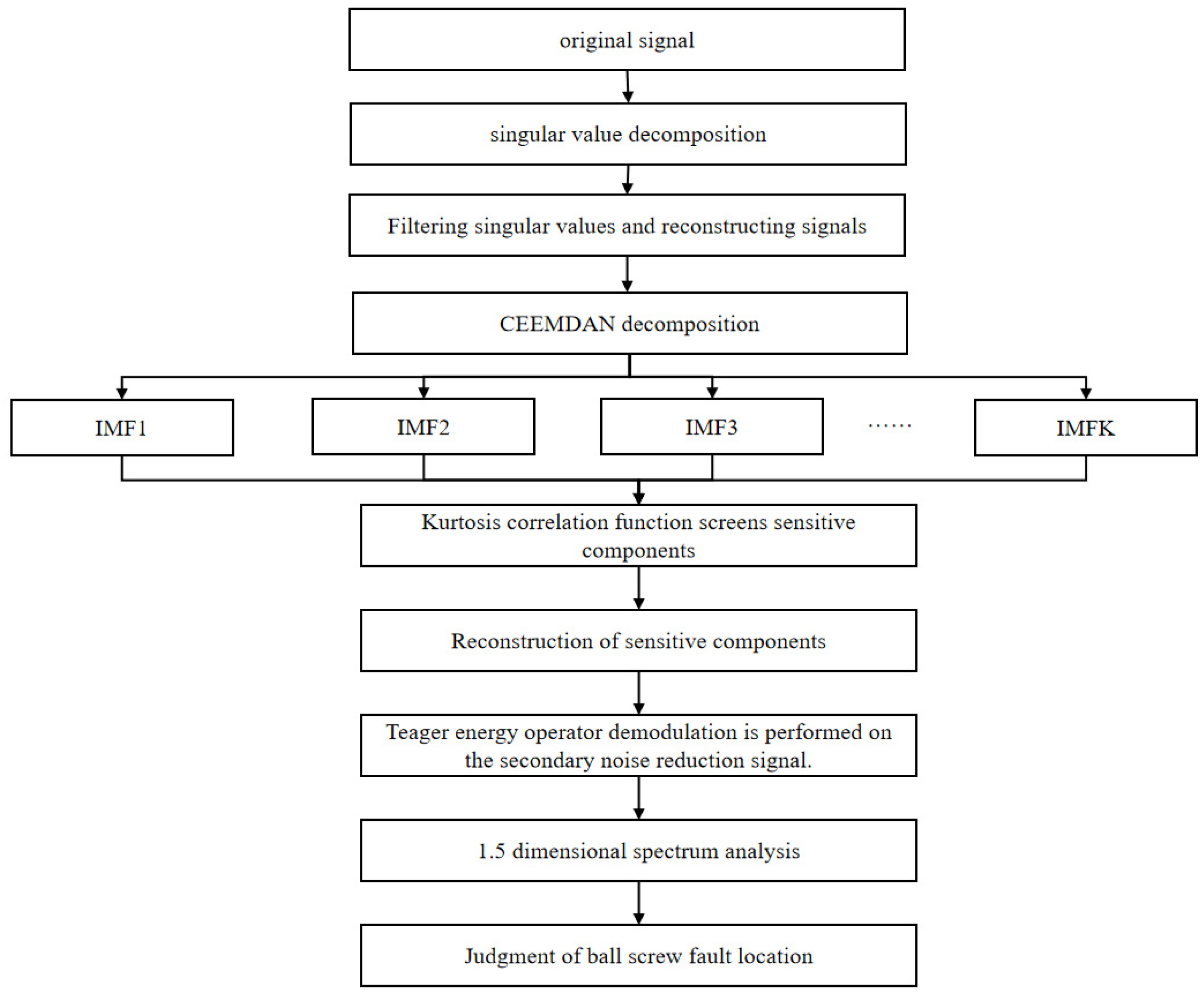
In this paper, an SVD-CEEMDAN-1.5DTES method is proposed to extract the fault signal characteristics of a ball screw under conditions of strong background noise interference and carry out a fault diagnosis [19]. The steps are as follows.

Step 1: For singular value decomposition of the original one-dimensional signal data, select and decompose several groups of singular values, compare and analyze the size of the singular values, and retain the larger singular values. The smaller singular values are set to zero, the signal is reconstructed, and the signal after noise reduction is restored.

Step 2: CEEMDAN decomposition is performed on the signal of the initial noise reduction to obtain several IMF component components. Because the kurtosis is particularly sensitive to the pulse impact signal, it is very effective for early ball screw fault detection. The expression is shown as Equation (12). The correlation between each IMF component and the original signal can be quantified by the correlation coefficient. The expression is shown as Equation (13). The sensitive components, which contain more fault information, are screened according to the kurtosis correlation function index, and the signal is reconstructed to complete the second noise reduction.

$$K=\frac{{\sum }_{i=1}^n(x_i-\overline{x}{)}^4}{(n-1){\sigma }^4}$$

(12)

$${\rho }_{XY}=\frac{E\left(\left(X-EX\right)\left(Y-EY\right)\right)}{\sqrt{D\left(X\right)}\sqrt{D\left(Y\right)}}$$

(13)

Here, $\overline{x}$ is the mean, and σ is the standard deviation. ρ_XY is the correlation coefficient between each component and the original signal, E is the expectation, and D is the variance. The kurtosis value of the original signal is taken as X and the kurtosis value of the IMF component is taken as Y, which is substituted into Equation (13) to obtain the size of the correlation coefficient.

Step 3: Teager energy operator demodulation is performed on the denoised signal, after which, 1.5D spectrum analysis is performed. The fault frequency extracted from the spectrum is compared with the fault frequency obtained from the theoretical calculation, and the fault location of the ball screw is determined.

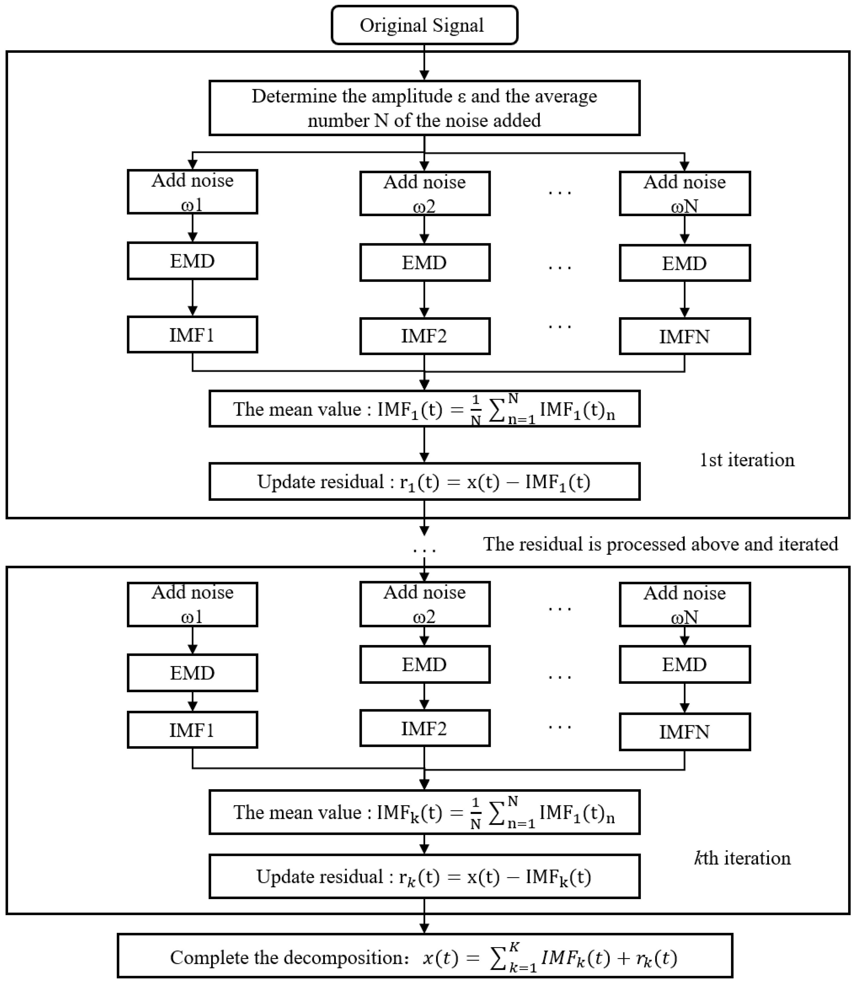
The specific steps of CEEMDAN decomposition are shown in Figure 2.

4. Simulation Signal Analysis

Ball Screw Simulation Signal Fault Diagnosis

In order to verify that the proposed method can accurately extract the characteristic frequency of the ball screw fault, first, the fault simulation signal is studied, then the periodic impact fault simulation signal of the ball screw is constructed. The mathematical formula of the vibration model is shown in Equation (14):

$$\left\{\begin{array}{l}\mathrm{x}\left(\mathrm{t}\right)=\mathrm{s}\left(\mathrm{t}\right)+\mathrm{n}\left(\mathrm{t}\right)={\sum }_{\mathrm{i}}{\mathrm{A}}_{\mathrm{i}}\mathrm{h}(\mathrm{t}-\mathrm{i}\mathrm{T})+\mathrm{n}\left(\mathrm{t}\right)\\ \mathrm{h}\left(\mathrm{t}\right)=\exp (-\mathrm{Ct})\cos \left(2\mathsf{\pi }{\mathrm{f}}_{\mathrm{n}}\mathrm{t}\right)\\ {\mathrm{A}}_{\mathrm{i}}=1+{\mathrm{A}}_0\cos \left(2\mathsf{\pi }{\mathrm{f}}_{\mathrm{r}}\mathrm{t}\right)\end{array}\right.$$

(14)

In the above formula, A₀ is the displacement constant, A₀ = 0.3; f_r is the frequency of the motor, f_r = 30; C is the attenuation coefficient, C = 700; f_n is the natural frequency, f_n = 3 kHz; h(t) is the impulse function; A_i is the amplitude of the impact signal; n(t) is the added Gaussian white noise, with a value of 4 dB; x(t) is the fault simulation signal after adding Gaussian white noise; t is the period of characteristic frequency, where the fault characteristic frequency $\mathrm{f}=1/\mathrm{T}=90\mathrm{Hz}$.

Comparing (a) and (b) in Figure 3, it can be seen that the time domain waveform with noise has become less obvious under the influence of noise, as shown in Figure 3c. Therefore, the signal needs to be processed.

This paper chooses to use the singular value decomposition noise reduction method. Firstly, singular value decomposition of the original one-dimensional signal data is carried out, and twelve groups of eigenvalues are selected and decomposed. Then, the size of each singular value and the corresponding eigenvectors are calculated. By analyzing the size of the singular value, several groups with larger singular values are selected. It can be seen from Figure 4 that the first two of the twelve eigenvalues, obtained by the singular value decomposition of the original signal, are relatively large, which will mainly reflect the useful signal. The third to the twelfth eigenvalues are smaller than the first two, which mainly reflect the noise. The singular values reflecting the noise are set to zero, and the signal is reconstructed to restore the signal after noise reduction.

Selecting the number of eigenvalues of SVD is a trade-off process, in which the balance between accuracy and computational efficiency needs to be considered. More eigenvalues can better retain the information of the original data, and can also provide more details and accuracy, so as to better describe the changes and patterns of the data. However, fewer eigenvalues can improve the efficiency of calculation. The computational complexity of singular value decomposition is proportional to the number of eigenvalues. Selecting an appropriate number of eigenvalues can increase the calculation speed and improve the efficiency of the algorithm. The motivation for selecting 12 eigenvalues is to maintain a balance between data accuracy and computational efficiency.

Figure 5 shows the signal frequency domain diagram after singular value decomposition and noise reduction. Comparing Figure 3c with Figure 5, it can be seen that the noise on both sides of the frequency domain image is obviously suppressed. Singular value decomposition denoising can remove part of the noise in the signal. However, it is still impossible to source effective fault information from the resulting spectrogram. Therefore, it is necessary to further reduce the noise.

The characteristics of CEEMDAN decomposition comprise gradually decomposing vibration signals of different frequencies, from high frequency to low frequency, but some pseudo-components and false components will be generated in the decomposition process. Therefore, it is necessary to filter the IMF components to remove some irrelevant components. The initial noise reduction signal is decomposed by CEEMDAN and a total of 13 IMF components are generated. The signal fault frequency component usually exists in the high-frequency part of the signal, and the remaining modal functions can be used as noise interference. Due to space limitations, only the first seven IMF components after decomposition are listed. The time domain waveform is shown in Figure 6.

Sensitive fault components are screened according to the kurtosis−correlation coefficient index. As shown in Figure 7, the first three components of the correlation coefficient contain more fault information; the kurtosis value generally shows a downward trend, indicating that the impact characteristics of the first several IMF components are obvious and that there is a greater possibility of failure. Considering the above two index values, the vibration signals of the first three components are reconstructed to complete the second noise reduction. The Teager energy operator is used to demodulate the vibration signal of the two noise reductions, then the 1.5D spectrum analysis is performed. From Figure 8, it can be seen that the fault characteristic frequency extraction method proposed in this paper can accurately extract the rotation frequency, the twice the rotation frequency, the fault characteristic frequency, and its 2 to 9 times frequency of the fault simulation signal, indicating that the singular value decomposition and CEEMDAN joint noise reduction can meet the requirements of noise reduction. The Teager energy operator can highlight the fault impact component, and the 1.5D spectrum can suppress the noise component well.

5. Measured Signal Analysis

The ball screw model GD4010 was selected for the test, and the process parameters are shown in

Table 1. The GD4010 process parameters of the ball screw pair.

Name	Screw Diameter	Ball Diameter	Contact Angle	Screw Lead Angle
unit	d0/mm	db/mm	α/°	λ/°
numerical value	40	5.953	45	4.55

.

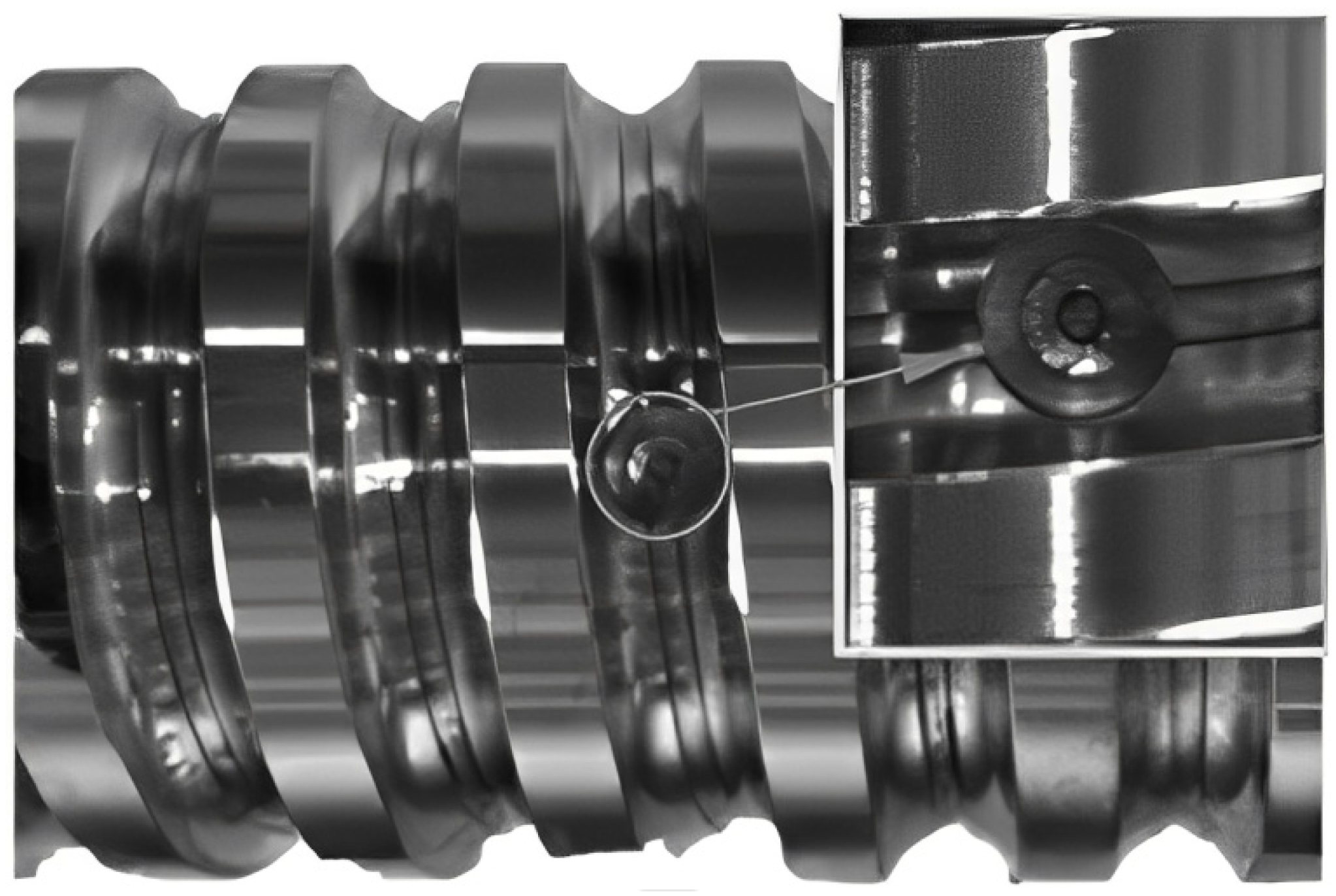
The fatigue pitting failure fault signal of a ball screw pair was analyzed and tested. Because the ball screw pair will undergo induction quenching heat treatment on the surface before leaving the factory, the hardness and wear resistance will be greatly improved. Therefore, it often takes some time to run in a new ball screw pair to the point of obvious pitting failure characteristics. In order to save testing time, EDM technology was used to create pits on the surface of the screw raceway to simulate the pitting failure state of the screw, as shown in Figure 9.

The frequency of the driving motor is f_r; if the pitting defect occurs in the nut raceway, the corresponding fault characteristic frequency is f_o; if the pitting defect appears in the screw raceway, the fault characteristic frequency is f_i [20], and the expression is as follows:

$$\left\{\begin{array}{l}{f}_r=\frac{n}{60}\\ f_o=\frac{\pi d_0{\omega }_s\left(1-{\gamma }^{\prime }\cos \alpha \right)}{2d_b}\\ f_i=\frac{\pi d_0{\omega }_s\left(1+{\gamma }^{\prime }\cos \alpha \right)}{2d_b}\end{array}\right.$$

(15)

where n is the motor speed, d_b is the ball diameter, d₀ is the nominal diameter of the screw, α is the contact angle of the ball with the nut and the screw, and ω_s is the derivative of the angular displacement generated by the screw rotation. Where ${\gamma }^{\prime }=d_b/2r_m$, rm is the vertical distance from the ball center to the screw center.

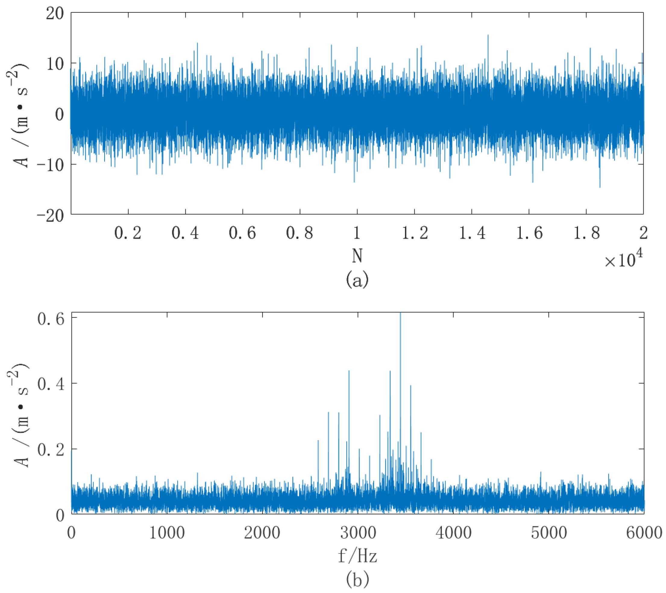
In order to verify the anti-noise performance of the method, Gaussian white noise with a signal-to-noise ratio of 14 dB was added to the original signal. The time-domain and frequency-domain diagrams of the denoised signal are shown in Figure 10 and Figure 11.

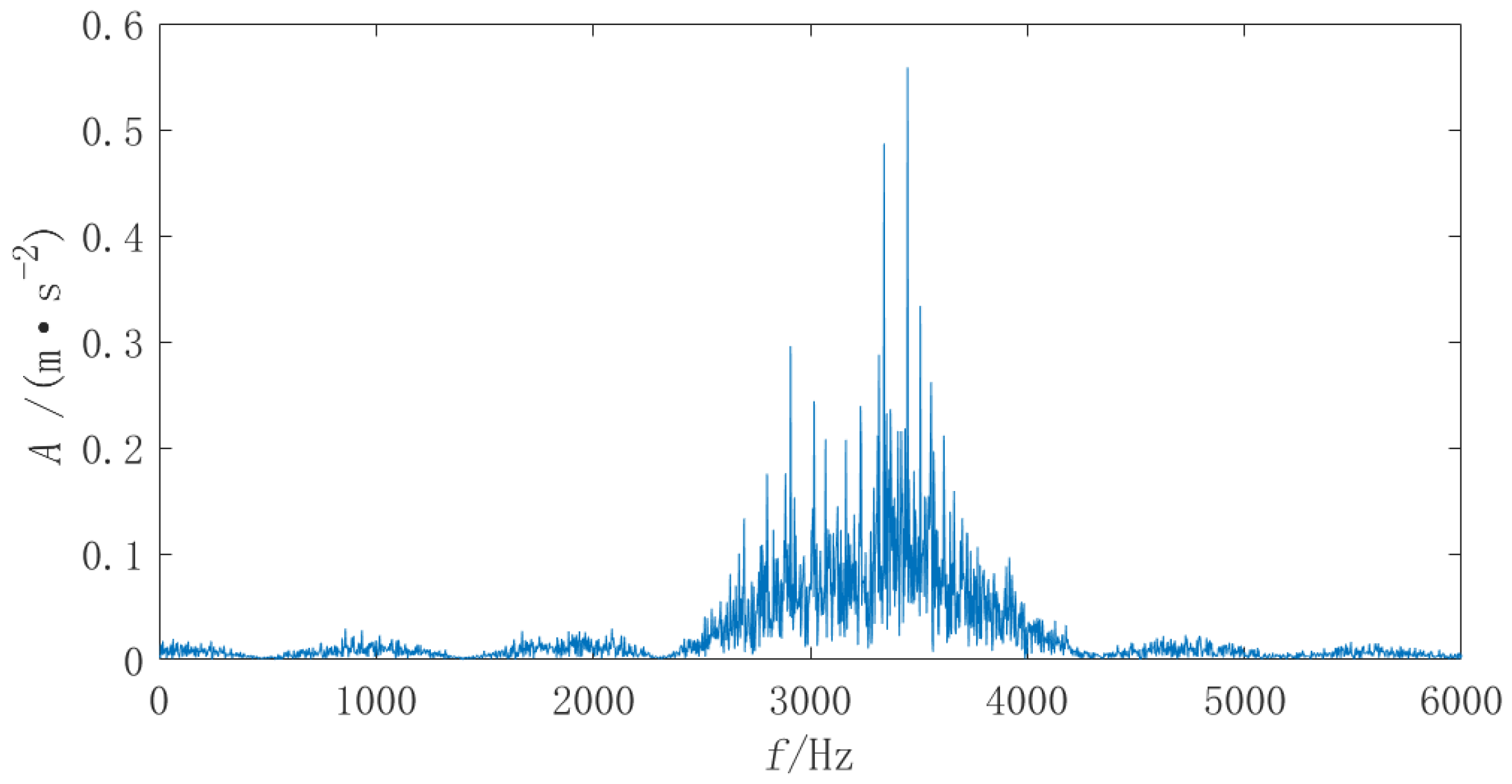
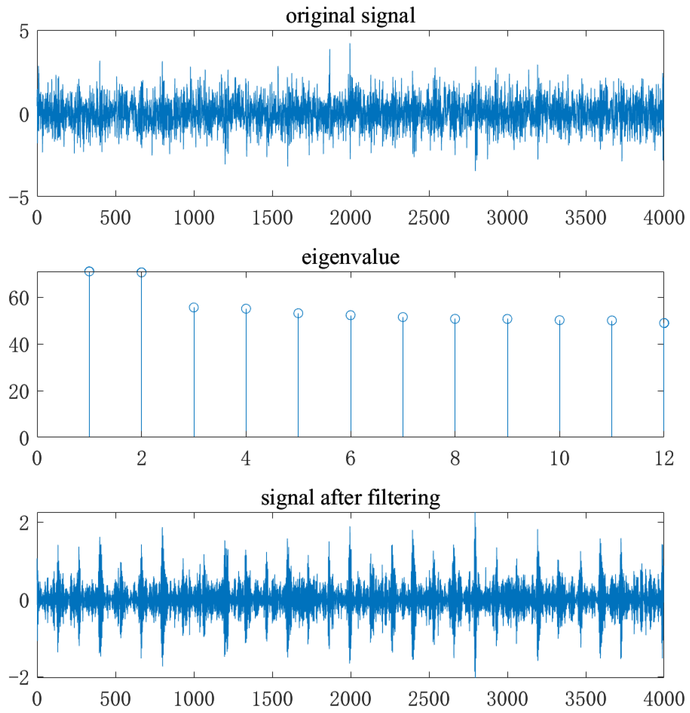
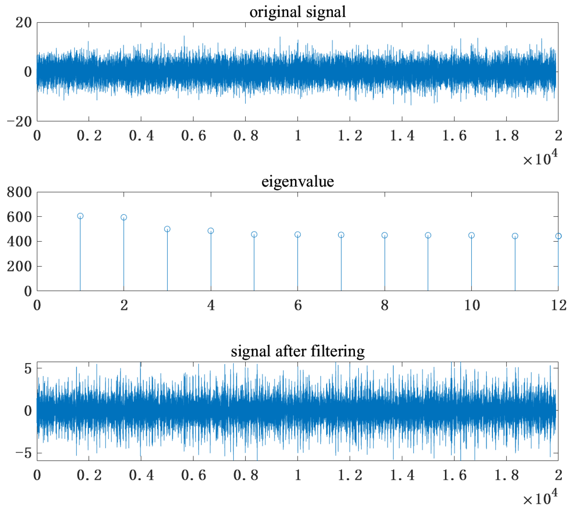
It can be seen from (a) in Figure 10 that there was a great deal of random noise interference, the signal was messy, and the impact characteristics have been completely annihilated. The fault characteristic frequency in frequency domain (b) in Figure 10 has migrated, and the fault characteristic frequency of the screw raceway could not be observed due to the influence of strong background noise. Therefore, it was necessary to denoise the signal. The wavelet packet was used to pre-denoise the ball screw raceway fault signal of the ball screw. Singular value decomposition of the signal was carried out, and a total of 12 singular values were decomposed. The singular values were filtered and then reconstructed. Each singular value that was calculated is shown in Figure 11. It can clearly be seen that the fault features were mainly concentrated in the first and second singular values. Therefore, the signal corresponding to the two singular values was reconstructed, which effectively removed other parts with less fault information and achieved a certain noise-reduction effect.

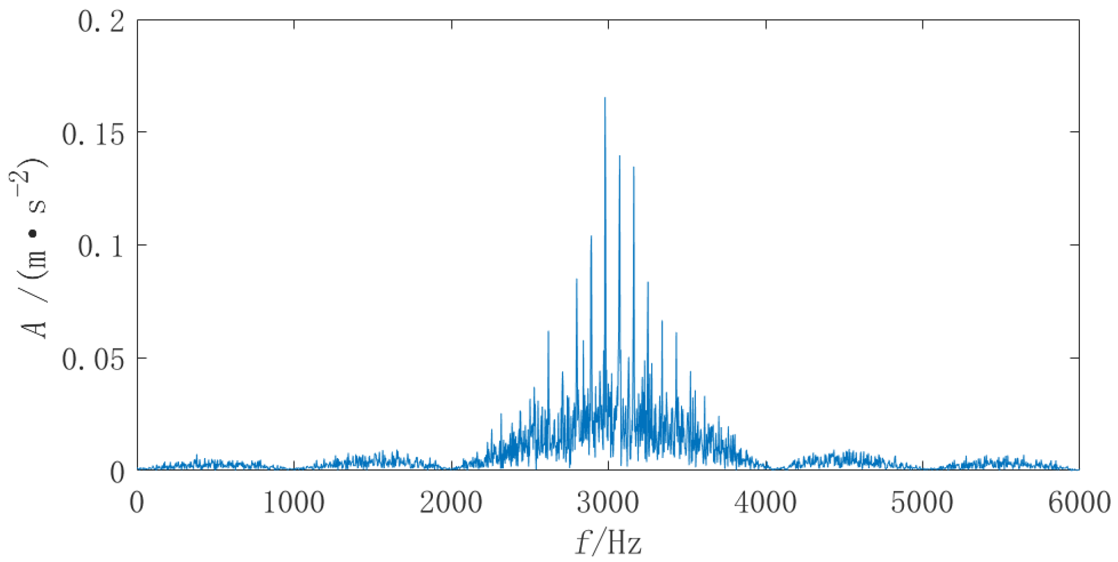
By comparing the original signal and the signal after filtering in Figure 11, it can be seen that a small part of the noise was removed after singular value decomposition; the impact characteristics were still not obvious, and the noise interference was very large. Comparing Figure 10 and Figure 12, it can be seen that the noise on both sides has been well suppressed, and the signal-to-noise ratio has been improved. However, the fault frequency cannot be identified from the spectrogram. Thus, the fault frequency of the screw cannot be extracted by relying solely on singular value decomposition noise reduction. Therefore, it is necessary to perform CEEMDAN decomposition on the initial noise reduction signal and then filter the sensitive components and reconstruct them for secondary noise reduction. A total of 13 IMF components were generated during the decomposition process, and only the first seven components are shown in Figure 13. The time-domain waveform of the first seven IMF components of CEEMDAN decomposition is shown in Figure 13.

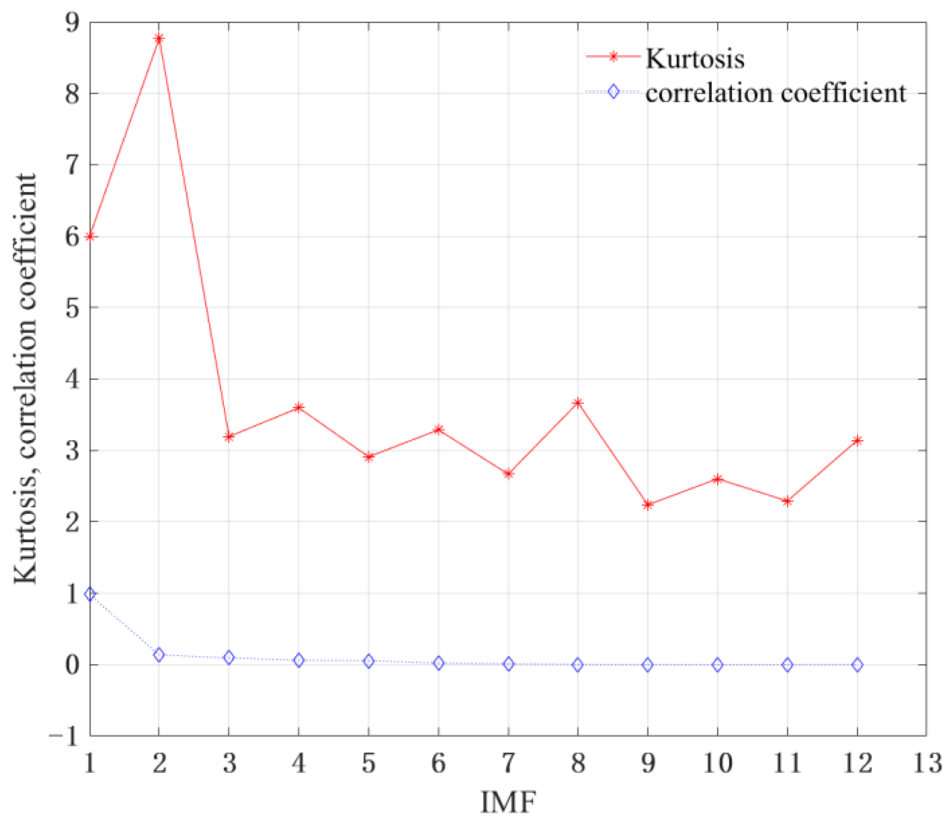
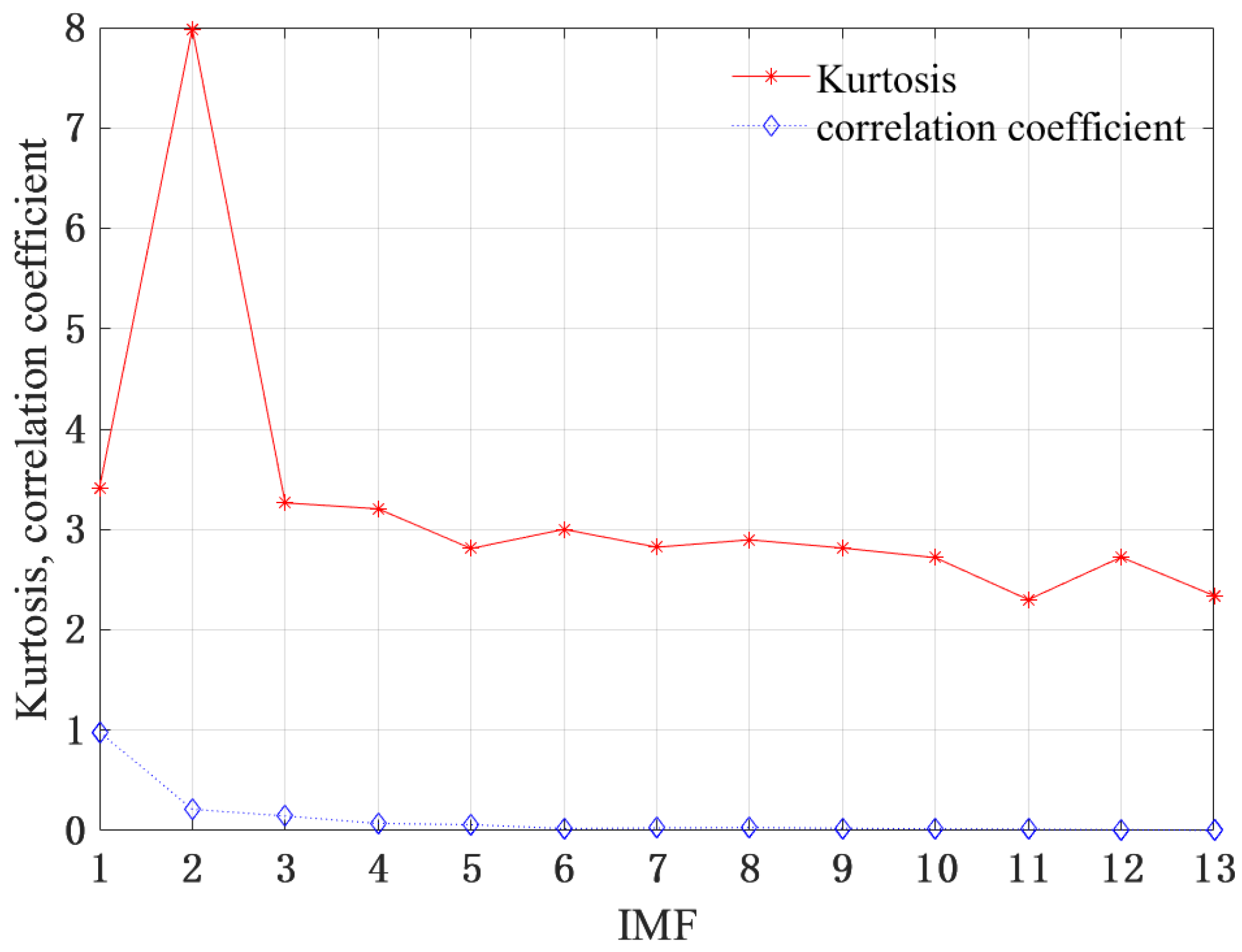
The sensitive components were screened, based on the set kurtosis−correlation coefficient criterion. It can be seen from Figure 14 that the correlation coefficient shows a downward trend as a whole, indicating that the first three components contain more fault information. The first and second components of kurtosis value are the largest, and the impact characteristics are obvious. Considered comprehensively, the vibration signals of the first three components were reconstructed to complete the secondary noise reduction processing.

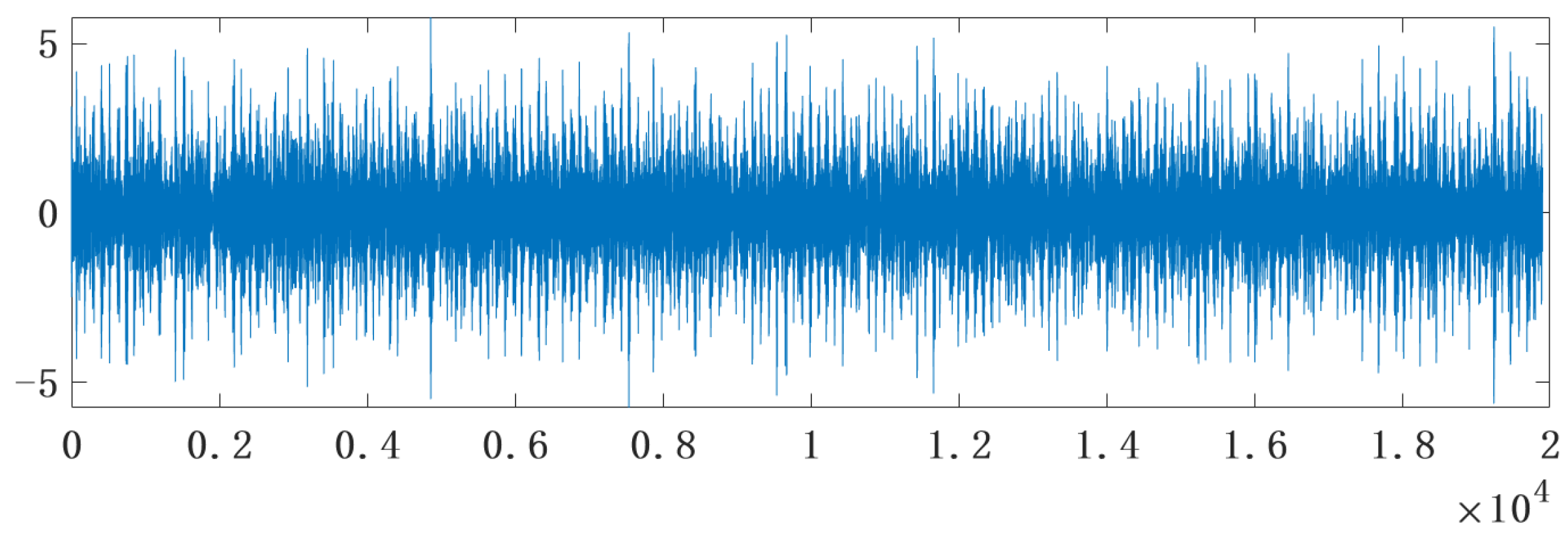
The first two IMF components after CEEMDAN decomposition were reconstructed; the reconstructed signal vibration image is shown in Figure 15. This is the final vibration signal image, which was extracted after two noise reductions.

In order to verify the effectiveness and accuracy of the method proposed in this chapter, the original signal was directly analyzed using 1.5DTES without noise reduction. Singular value decomposition, CEEMDAN and Teager energy spectrum analysis were used to compare with the proposed method. The results are as follows.

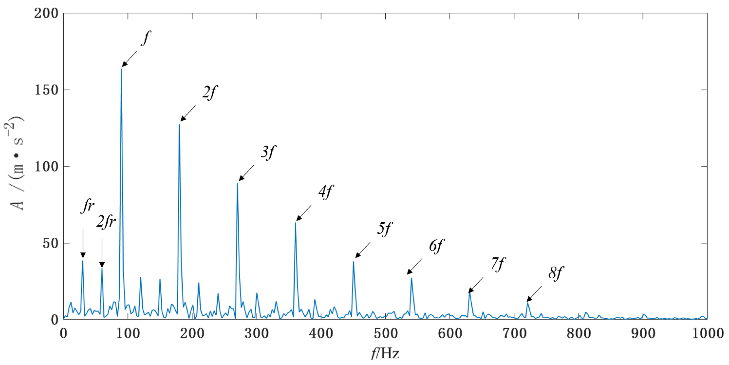
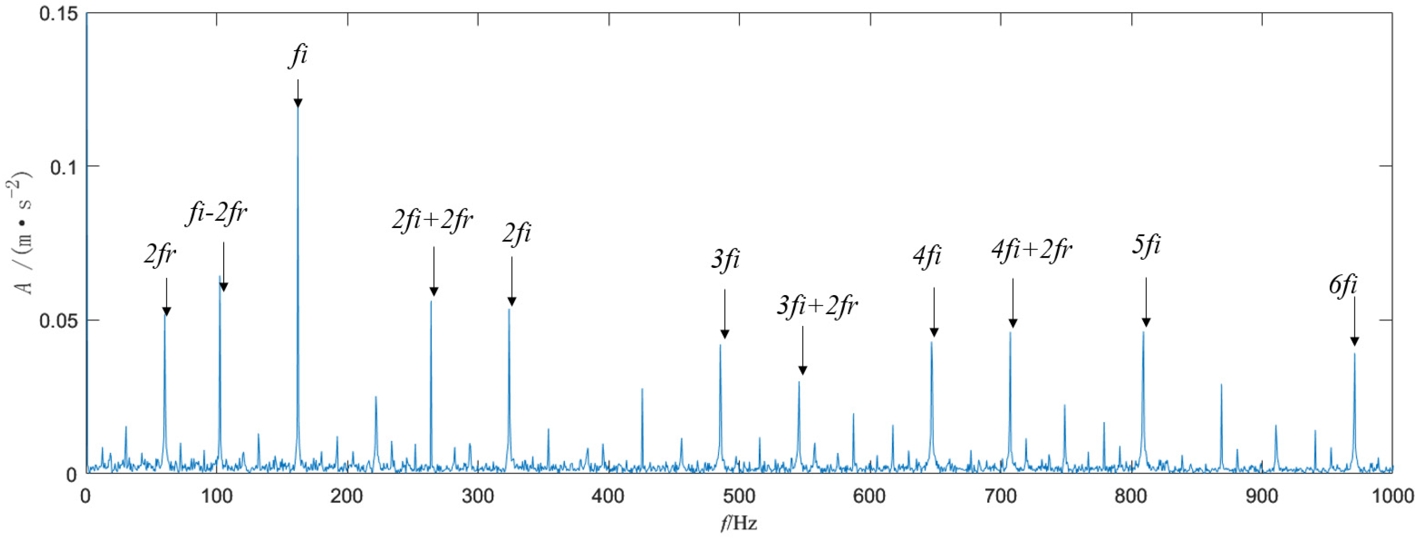
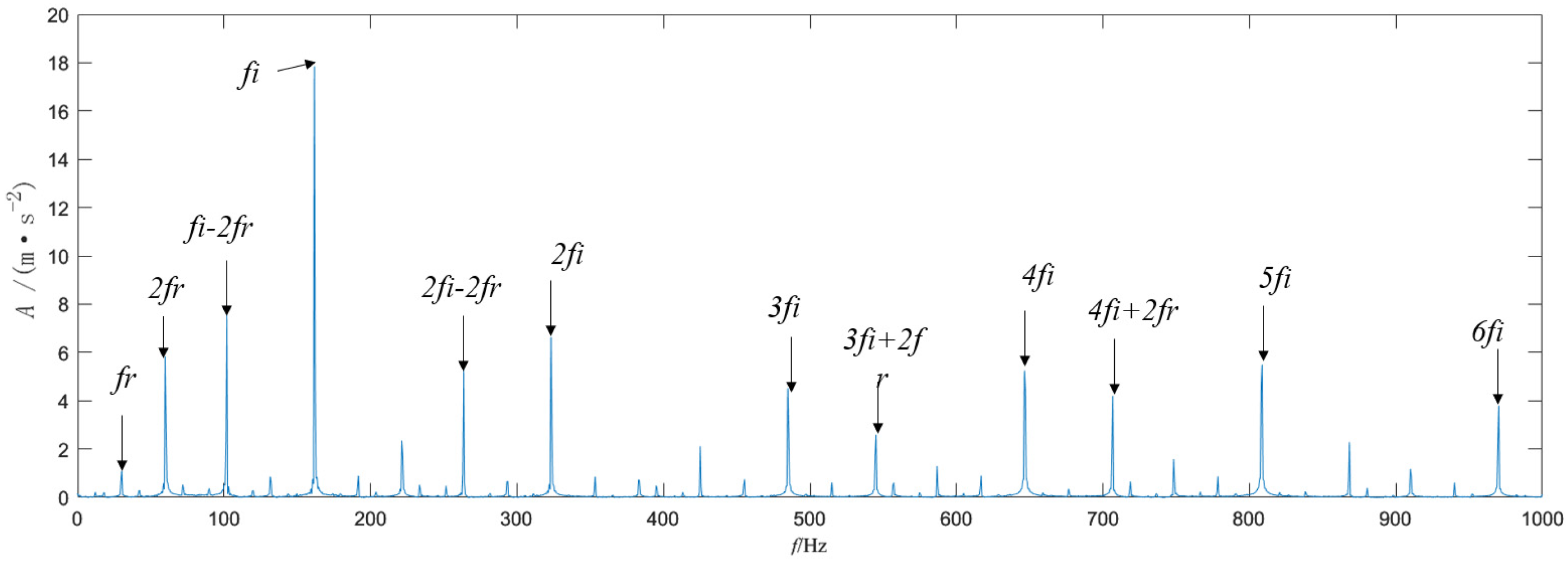
In Figure 16, the fault signal of the ball screw is analyzed using 1.5DTES, which can only identify double the failure frequency. The noise interference is great, and the extraction effect is poor. From Figure 17 and Figure 18, it can be concluded that the Teager energy spectrum and 1.5DTES can extract the 2-times rotation frequency, the fault characteristic frequency, and the 2 to 6-times frequency, and the sideband of the rotation frequency modulation can be clearly observed. It has been comprehensively determined that there is a fault in the screw raceway of the ball screw. Comparing Figure 17 and Figure 18, it is clear that the rotation frequency and twice rotation frequency can be extracted from Figure 18, while only a twice the rotation frequency can be identified in Figure 17. In addition, by combining the Teager energy operator with the 1.5D spectrum, the noise component is significantly lower, the spectral line is more prominent, and the overall effect is better. This shows that the 1.5D spectrum has a good inhibitory effect on noise. The frequency value extracted from Figure 18 is 161.6 Hz, and the theoretical fault frequency is 161.74 Hz. These values are very close; Therefore, it is possible to prove that the extraction is very accurate. This also verifies that the method used in this chapter can accurately extract the frequency of the screw raceway fault signal.

Wavelet denoising and singular value denoising have certain effects on ball screw fault diagnosis. The wavelet denoising method is widely used in the field of signal processing. It can effectively remove the noise and interference from the signal and retain the important information of the signal. In the fault diagnosis of ball screws, wavelet denoising can remove the noise and interference in the vibration signal, improve the signal-to-noise ratio of the signal, and is conducive to the accurate diagnosis of ball screw faults. Singular value denoising is employed to decompose the signal into different parts by singular value decomposition and to remove the noise and interference contained therein. In ball screw fault diagnosis, singular value denoising can decompose the vibration signal, extract the principal component of the signal, and avoid the influence of noise and interference on the fault diagnosis. Therefore, a wavelet regression network (WRN) was used to denoise the original signal for the first time, and the results are compared with the results of this method.

Ren Liang et al. [21] used the singular spectrum decomposition algorithm to decompose the fault signal and reconstructed the decomposed signal according to the time domain cross-correlation criterion. Subsequently, the whale optimization algorithm (WOA) was used to optimize the parameters of VMD, and the reconstructed signal was decomposed by the parameter-optimized VMD. Working according to the kurtosis index, the fault characteristic signal was extracted from the decomposed intrinsic mode function. In order to verify the superiority of the proposed method, Ren Liang’s method was used to analyze the measured fault signal with 14 dB of Gaussian white noise, and the results were compared with the proposed method. The results of the above two methods are shown in

Table 2. The kurtosis correlation coefficient of each IMF.

IMF	1	2	3	4	5
WRN-CEEMDAN	0.9761	0.2690	0.0572	0.0071	0.0028
SVD-CEEMDAN	0.9860	0.3396	0.0511	0.1790	0.0373
SVD-WOA-VMD	0.5598	0.4701	0.5004	0.4768	0.3937

.

6. Conclusions

(1)

In this paper, a fault diagnosis method for ball screw faults based on the SVD-CEEMDAN-1.5DTES algorithm is proposed, which can effectively extract the fault characteristics of a ball screw in a strong background noise environment and accurately diagnose the fault in a ball screw.

(2)

The SVD algorithm can effectively suppress noise interference. The application of the 1.5-dimensional envelope spectrum offers more advantages than the traditional envelope spectrum. It can accurately extract the weak fault information generated by the ball screw under the interference of strong noise, and can effectively suppress the background noise. The diagnosis results, which are based on the SVD-CEEMDAN-1.5DTES algorithm, are better than those with the SVD-CEEMDAN Teager algorithm.

(3)

Within a strong background noise environment, the fault diagnosis results for the ball screw based on the SVD-CEEMDAN denoising algorithm are better than those based on the WRN-CEEMDAN algorithm and SVD-WOA-VMD algorithm. In future research, this method will be further optimized.

References

1. Zhang, Y.; Lc, Y.; Ge, M. Complementary ensemble adaptive local iterative filtering and its application to rolling bearing fault diagnosis. IEEE Access 2021, 9, 47275–47293. [Google Scholar] [CrossRef]
2. Xiangnan, L.; Xuezhi, Z.; Wenbin, S. Feature extraction of rolling bearing fault impact in strong background noise vibration signal. J. Vib. Eng. 2021, 34, 202–210. [Google Scholar]
3. Wang, Z.; Li, Y.; Dong, L.; Li, Y.; Du, W. A Rul Prediction of Bearing Using Fusion Network through Feature Cross Weighting. Meas. Sci. Technol. 2023, 34, 105908. [Google Scholar] [CrossRef]
4. Shi, Y.; Zhang, Q. Bearing Fault Diagnosis Based on Wavelet Denoising and XGBoost Fusion Feature Selection. Available online: http://kns.cnki.net/kcms/detail/41.1148.TH.20220421.1700.002.html (accessed on 4 October 2023).
5. Wu, Y.; Wang, J.; Xu, X.; Jiang, Z. Application of FastICA combined noise reduction method based on wavelet analysis in fault diagnosis of rolling bearings. China Mech. Eng. 2017, 28, 2183–2188+2197. [Google Scholar]
6. Cai, K.; Wang, L.; Xu, Z. Feature extraction and analysis of weak bearing faults based on SVD and VMD. Comb. Mach. Tool Autom. Mach. Technol. 2022, 578, 70–73+78. [Google Scholar]
7. Huang, N.E.; Shen, Z.; Long, S.R.; Wu, M.C.; Shih, H.H.; Zheng, Q.; Yen, N.C.; Tung, C.C.; Liu, H.H. The empirical mode decomposition and the Hilbert spectrum for nonlinear and non-stationary time series analysis. Proc. Math. Phys. Eng. Sci. 1998, 454, 903–995. [Google Scholar] [CrossRef]
8. Torres, M.E.; Colominas, M.A.; Schlotthauer, G.; Flandrin, P. A complete ensemble empirical mode decomposition with adaptive noise. In Proceedings of the IEEE International Conference on Acoustics, Speech and Signal Processing, Prague, Czech Republic, 22–27 May 2011; IEEE: New York, NY, USA, 2011; pp. 4144–4147. [Google Scholar]
9. Wang, Z.; Zhao, W.; Li, Y.; Dong, L.; Wang, J.; Du, W.; Jiang, X. Adaptive staged RUL prediction of rolling bearing. Measurement 2023, 222, 113478. [Google Scholar] [CrossRef]
10. Liu, L.; Wei, Y.; Song, X.; Zhang, L. Fault Diagnosis of Wind Turbine Bearings Based on CEEMDAN-GWO-KELM. Energies 2022, 16, 48. [Google Scholar] [CrossRef]
11. Yan, H.; Zhou, H.; Wang, Y. Combining the synchrosqueezing generalized S-transform of variational mode decomposition with the Teager–Kaiser energy operator to calculate the attenuation gradient for identifying oil and gas reservoirs. Acta Geophys. 2022, 71, 795–812. [Google Scholar] [CrossRef]
12. Tang, G.; Xue, G.; Wang, X.; Ding, A. Rolling bearing fault diagnosis based on multivariate variational mode decomposition and 1.5-dimensional spectrum. Bearings 2022, 12, 74–82. [Google Scholar]
13. Dai, L.; Cao, W.; Yi, S.; Wang, L. Damage identification of concrete structures based on WPT-SVD and GA-BPNN. J. Zhejiang Univ. 2023, 57, 100–110+132. [Google Scholar]
14. Qi, L.; Shen, Z.; Guo, Q.; Wang, Y.; Mykola, K. Chirp Rates Estimation for Multiple LFM Signals by DPT-SVD. Circuits Syst. Signal Process. 2022, 42, 2804–2827. [Google Scholar] [CrossRef]
15. He, Z.; Li, J.; Liu, S.; Qin, Z. CEEMD-VMD combined with parameter optimization SVM for roller bearing fault diagnosis. Mech. Sci. Technol. 1–7.
16. Kaiser, J.F. Some useful properties of Teager’s energy operators. In Proceedings of the IEEE International Conference on Acoustics, Speech, and Signal Processing, Minneapolis, MN, USA, 27–30 April 1993; Volume 3, pp. 149–152. [Google Scholar]
17. Wang, H.; Shan, C.; Meng, J.; Chen, G.; Wu, L. A composite fault diagnosis method for rolling bearings based on Autogram resonance demodulation and 1.5-dimensional spectrum. J. Vib. Eng. 2022, 35, 1541–1551. [Google Scholar]
18. Zhu, Y.; Guan, L. Gearbox fault diagnosis based on fast spectral kurtosis and 1.5-dimensional spectrum. Baogang Technol. 2020, 46, 67–69. [Google Scholar]
19. Zhou, Z. Machine Learning; Tsinghua University Press: Beijing, China, 2016. [Google Scholar]
20. Nie, C.; Zhou, C.; Liu, D.; Feng, H.; Wang, Z.; Ou, Y. Application of HHT-SVM in fatigue pitting failure diagnosis of ball screw pair. Comb. Mach. Tool Autom. Mach. Technol. 2020, 12, 80–84+89. [Google Scholar]
21. Ren, L.; Zhen, L.; Zhao, Y.; Dong, Q.; Zhang, Y. Rolling bearing fault diagnosis under strong background noise environment based on SSA-VMD-MCKD. Vib. Shock. 2023, 42, 217–226. [Google Scholar]
Figure 1. The flow chart of CEEMDAN decomposition.
Actuators 12 00416 g001
Figure 2. Ball screw fault diagnosis flow chart.
Actuators 12 00416 g002
Figure 3. Simulation signal diagram. (a) Simulation signal time domain diagram; (b) The time domain diagram of the simulated signal after adding noise; (c) The frequency domain diagram of the simulated signal after adding noise.
Actuators 12 00416 g003
Figure 4. De-noising of singular value decomposition.
Actuators 12 00416 g004
Figure 5. Signal frequency domain diagram after preliminary noise reduction.
Actuators 12 00416 g005
Figure 6. CEEMDAN decomposition diagram.
Actuators 12 00416 g006
Figure 7. Kurtosis–correlation coefficient index.
Actuators 12 00416 g007
Figure 8. Simulation signal, shown in a 1.5DTES diagram.
Actuators 12 00416 g008
Figure 9. Electrospark preparation: the pitting effect diagram.
Actuators 12 00416 g009
Figure 10. The experimental fault signal diagram. (a) Ball screw nut fault time domain diagram; (b) Ball screw nut fault frequency domain diagram.
Actuators 12 00416 g010
Figure 11. Singular Value Decomposition of Measured Signal.
Actuators 12 00416 g011
Figure 12. Frequency domain diagram of the experimental fault signal after initial noise reduction.
Actuators 12 00416 g012
Figure 13. CEEMDAN decomposition diagram of the experimental signal after noise reduction.
Actuators 12 00416 g013
Figure 14. Experimental signal, showing the kurtosis–correlation coefficient index.
Actuators 12 00416 g014
Figure 15. The IMF component’s reconstructed signal image.
Actuators 12 00416 g015
Figure 16. The 1.5DTES analysis of the un-noised signal.
Actuators 12 00416 g016
Figure 17. Teager energy spectrum analysis of the de-noising signal.
Actuators 12 00416 g017
Figure 18. Noise reduction processing signal, as shown by the 1.5DTES analysis.
Actuators 12 00416 g018