Modeling and Fault Simulation of a New Double-Redundancy Electro-Hydraulic Servo Valve Based on AMESim

Abstract

The feedback spring rod of the armature assembly was eliminated in the double-redundancy electro-hydraulic servo valve (DREHSV), which employed a redundant design in contrast to the typical double-nozzle flapper electro-hydraulic servo valve (DNFEHSV). The pilot stage was mainly composed of four torque motors, and the double-system spool was adopted in the power stage. Consequently, the difficulty of spool displacement control was increased. By artificially changing the structural parameters of the simulation model in accordance with the theoretical analysis through AMESim, this paper aimed to study the dynamics and static characteristics of the DREHSV. The advantage of redundant design was further demonstrated by disconnecting working coils and setting the different worn parts of the spool. On the test bench, the necessary experiments were performed. Through simulation, it was discovered that when the clogged degree of the nozzle is increased, the zero bias value increases, the pressure and flow gain remain unchanged, and the internal leakage decreases. The pressure gain changes very little, the flow gain close to the zero position grows, the zero leakage increases significantly, and the pilot stage leakage changes very little as a result of the wear of the spool throttling edge. The basic consistency between the simulation curves and the experimental findings serve to validate the accuracy of the AMESim model. The findings can serve as a theoretical guide for the design, debugging, and maintenance of the DREHSV. The simulation model is also capable of producing a large amount of sample data for DREHSV fault diagnosis using a neural network.

1. Introduction

The electro-hydraulic servo valve (EHSV) is widely used in aviation, aerospace, and other fields [1]. With the development of aviation and aerospace, the EHSV has been upgraded relying on redundancy technology, and its reliability has greatly improved [2].

The common pilot stage of the EHSV is the double-nozzle flapper valve. Numerous academics have carried out modeling investigations on the DNFEHSV and the valve created using redundancy technology in recent years, and they have produced fruitful research findings.

To accomplish pilot control in the EHSV, Anderson et al. [3] employed two slide valves rather than a single slide valve. The feedback spring rod of the armature assembly is no longer required, improving manufacturing precision and lowering production costs. Through mathematical modeling, Chen et al. [4] established the static and dynamic characteristic equations for the single-stage DNFEHSV, and, in order to address the imprecision of the Taylor expansion local linearization approach, Mu et al. [5] constructed the DNFEHSV model while taking nonlinear parameters like the flow at the nozzle into consideration. Wang [6] studied the effects of the throttling edge fillet and radial clearance on the zero position characteristics of the three-stage EHSV by AMESim, and the simulation was used to assess how the degree of orifice clogging and the excessive oil–gas content affected the dynamic and static characteristics. The magnetic resistance of the permanent magnet and the magnetic permeator, as well as the magnetic leakage of the permanent magnet, were all considered in Liu’s [7] determination of the electromagnetic torque linearized expression of the torque motor. The calculation formulas for the spring stiffness and the electromagnetic torque coefficient were modified. Wang et al. [8] conducted the armature assembly sub-model by AMESet, and the DNFEHSV AMESim simulation model was established. Gordic et al. [9,10] established the EHSV simulation model with Simulink and analyzed the influences of zero gap length and coil turns. Li et al. [11] established the DNFEHSV simulation model by AMESim and analyzed the effects of common faults. Li [12] built the DNFEHSV multidisciplinary physical model through the Simcape Modeling Toolbox in Simulink. The model was highly precise and without complicated mathematical formulas. Shi [13] established the DNFEHSV simulation model by AMESim and proposed the PSO-CG-BP neural network model. It could be used in the field of fault diagnosis for the EHSV. The above-mentioned investigators conducted a simulation modeling study on the EHSV using AMESim or MATLAB, developed a trustworthy theoretical simulation model, and analyzed the impact of different settings on the performance of the servo valve. But since these simulation models are designed to simulate the conventional DNFEHSV, it is quite easy to control displacement and match parameters for power stage four-side slide valves. Yan et al. [14] developed a theoretical model for the triplex-redundancy EHSV and examined its dynamic and static properties using Simulink and AMESim, respectively. For a 2D servo valve, Yan [15] created a double-redundancy controller that allowed for a free changeover between controllers in the event of a problem. Aiming for a high-power thrust vector control for the future heavy launch vehicle, Chen et al. [16]. proposed a high-power redundant Electro-Hydrostatic Actuators (EHA) technical program. Adopting an advanced modular design, the EHA can realize a high-power output with a parallel connection of servomotor pumps with good dynamic performance and a high power-to-weight ratio, which verifies the technical feasibility of the EHA with higher redundancy levels, such as three or four redundancy levels. Han et al. [17]. designed a control system through the utilization of a Q-filter-based disturbance observer (DOB), which could eliminate the force-fighting phenomena and respond effectively to unexpected disturbances in redundant actuators. The simulation results confirmed the effectiveness and reliability of the method in accurately observing and responding to the force-fighting phenomenon that occurs in the redundant driving device. Based on the redundancy theories, the researchers created the simulation model and evaluated its accuracy. Additionally, they computed the transfer function of the EHSV using redundancy architecture, which is suitable for DNFEHSV with redundant design in the pilot stage but not in the power stage. However, the DREHSV features a pilot stage composed of two double-redundancy double nozzle flapper valves, and the double-system power stage slide valve is controlled by a total of four torque motors; therefore, the inferred transfer function is not applicable to the DREHSV. The double-system slide valve, four sets of piston bushes, and a four-redundancy displacement sensor (LVDT) make up the power stage. The oil inlet and outlet of the slide valve have rectangular holes rather than the more common round ones. The control difficulty of the DREHSV is sharply increased. In addition, the double redundancy actuator studied is mainly driven by servomotor pumps, and there are few studies on adapting the DREHSV to driving. Therefore, this paper mainly adopts AMESim to carry out simulation modeling research on the DREHSV and indirectly introduces the double redundancy actuator driven by the DREHSV to verify the advantage of the redundant design for the power stage.

Because there is not an appropriate sub-model in AMESim, the armature assembly sub-model is created by AMESet with C-code in order to create the simulation model to analyze the performance of the DREHSV. Through theoretical study, the double-system slide valve model is built, and then the DREHSV simulation model is established. Through simulation and experimentation, dynamic and static characteristic curves are generated. The effects of different faults on the performance are analyzed by AMESim, and the advantage of redundant design is verified, which could provide a reference for the design, debugging, and maintenance of the DREHSV. Abundant sample data can be generated by the model for the fault diagnosis of the valve.

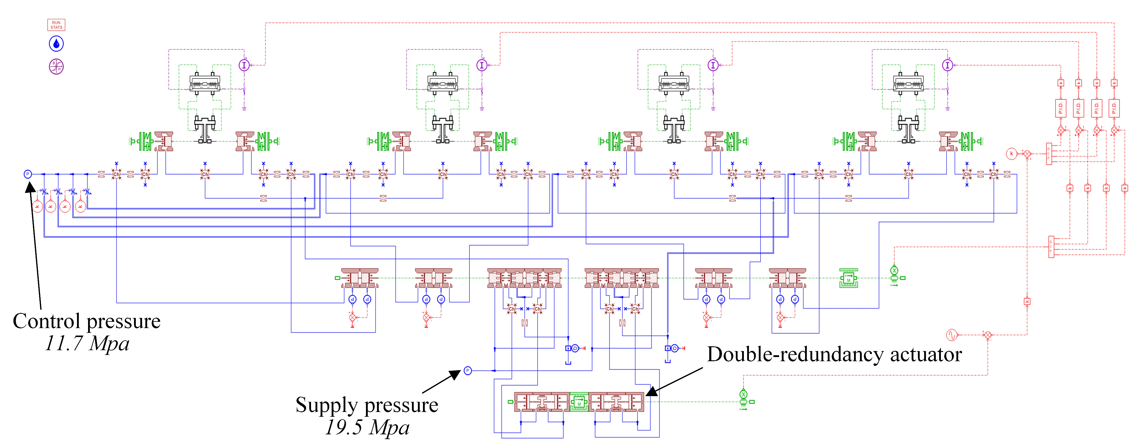
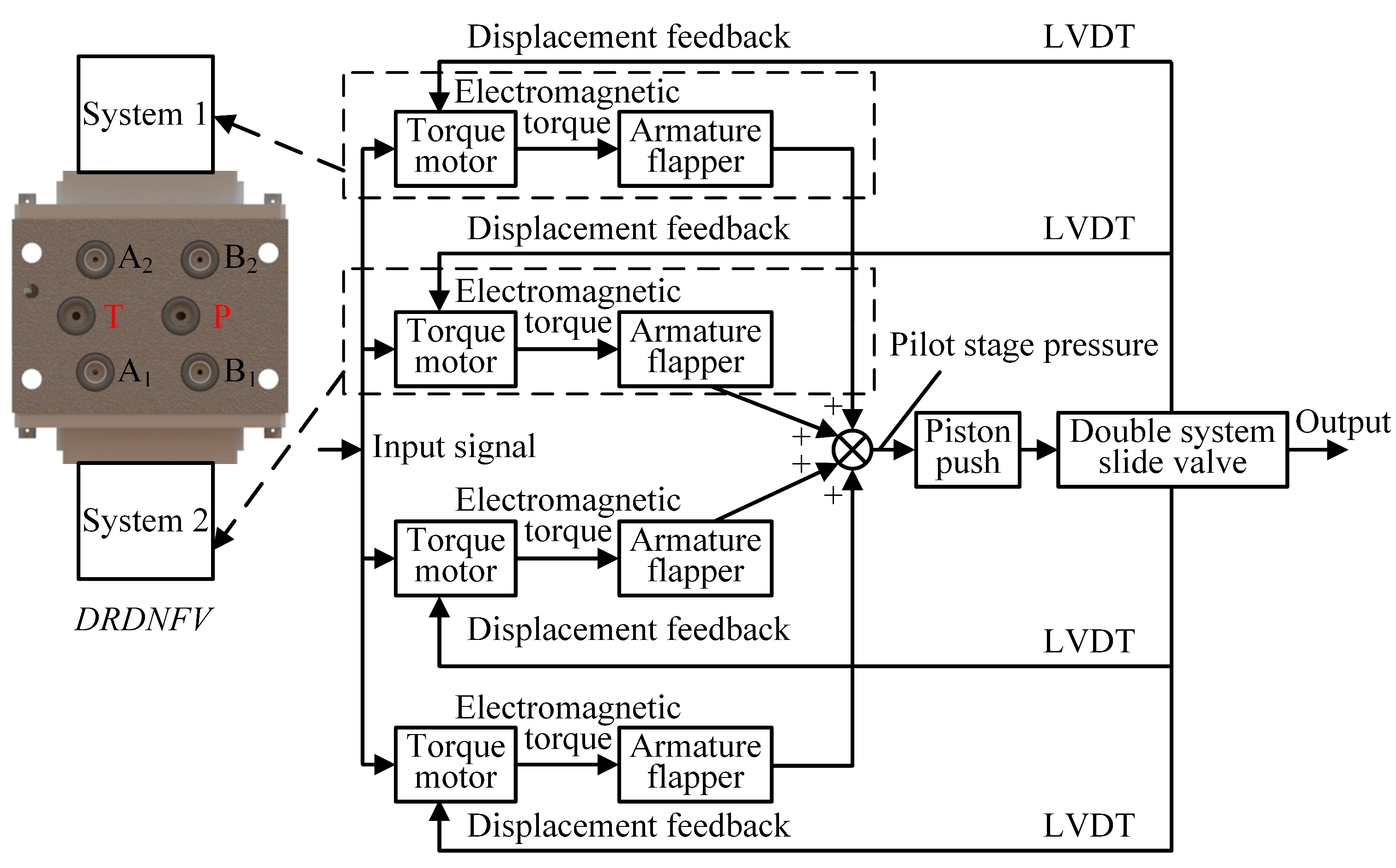
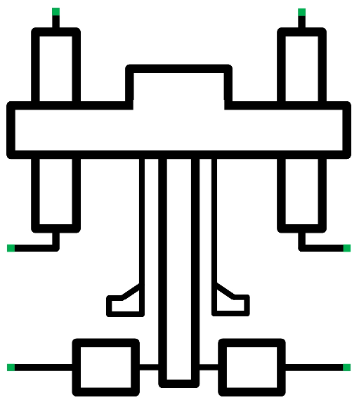
2. Working Principles

According to Figure 1, under the action of the input signal, four sets of the armature assembly of two DRDNFVs are deflected. The DRDNFV includes two sets of independent systems, and each system includes a torque motor, an armature, two nozzles, and other components. Four pairs of differential pressures generated by two DRDNFVs can move the four pistons at the two ends of the power stage. Therefore, when one system fails, the other can still continue to feedback and control the double system spool to make the valve work normally.

The double-system spool moves when the four pistons move because it is connected to the flexible rod with the four pistons. The double-system spool, which controls the motion of the double-system actuator, distributes the system flow. The spool displacement signal is transmitted to the signal input of the torque motor by the four redundancy linear variable displacement transducers (LVDTs) at the right end of the spool to form the closed-loop control.

3. DREHSV Modeling

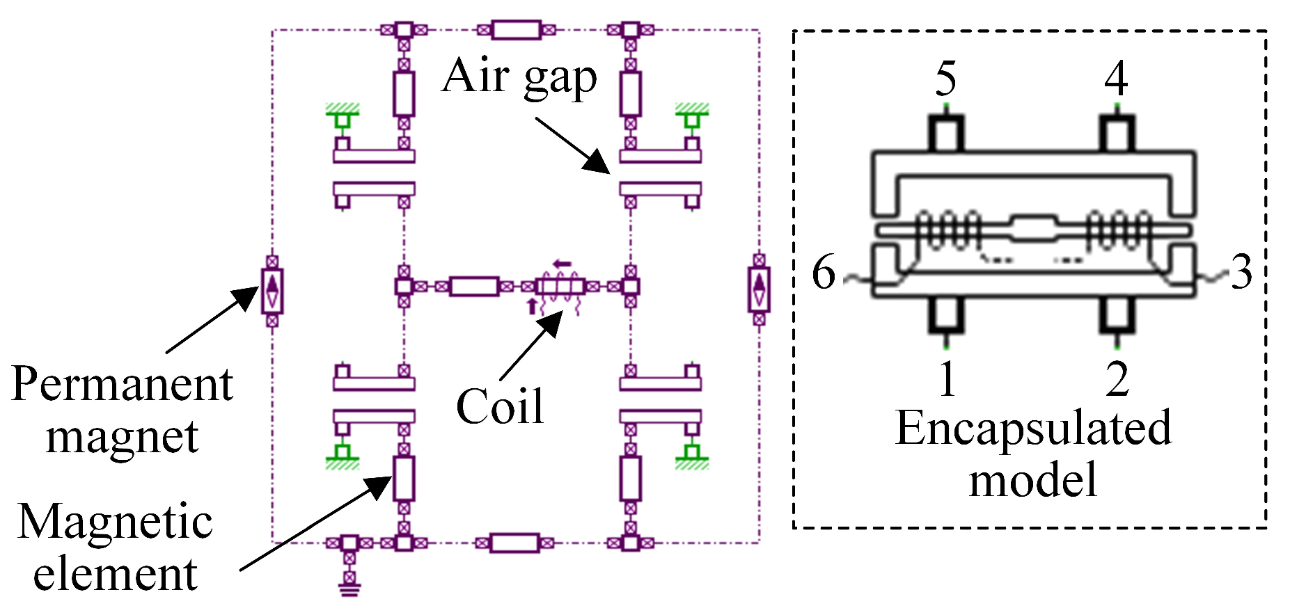
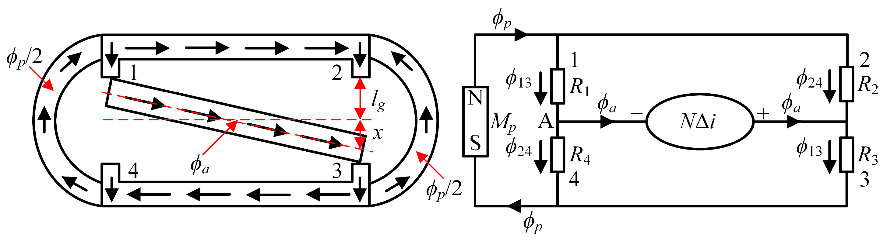
3.1. Torque Motor Modeling

A torque motor is an electric–mechanical conversion device that uses electromagnetic action to convert a current signal into the appropriate mechanical motion.

The permanent magnet moving-iron torque motor utilized in the DREHSV is made up of coils, permanent magnets, and magnetic elements, as shown in Figure 2. It could be streamlined, as illustrated in Figure 3, by ignoring leakage flux, magnetic materials, and the resistance of the non-working air gaps [18,19].

According to Figure 3, the magnetic flux in the four air gaps is equal in the initial condition and the total torque is zero; therefore, the armature does not deflect. When a command signal is applied, the total torque is not zero, causing the armature and spring tube to deflect.

The resistance of each operational air gap is displayed as follows, while the armature is in the middle position:

$$R_0=\frac{l_g}{{\mu }_0{A}_g}$$

(1)

where l_g is the length of each working air gap when the armature is in the middle position, μ₀ is the magnetic permeability of air, and A_g is the area of the magnetic pole surface.

The magnetoresistances R₁ and R₃ of the working air gaps 1 and 3 and R₂ and R₄ of the working air gaps 2 and 4 are the same, assuming that the armature deflects x to the right since the magnetic circuit is symmetric.

$$\begin{array}{l}{R}_1=R_3=\frac{l_{\mathrm{g}}-x}{{\mu }_0{A}_{\mathrm{g}}}=R_0\left(1-\frac{x}{l_{\mathrm{g}}}\right)\\ R_2=R_4=\frac{l_{\mathrm{g}}+x}{{\mu }_0{A}_{\mathrm{g}}}=R_0\left(1+\frac{x}{l_{\mathrm{g}}}\right)\end{array}$$

(2)

The balance equation of the magnetomotive force is shown as follows:

$$\left\{\begin{array}{c}{R}_1{\varphi }_{13}-R_2{\varphi }_{24}=N\Delta i\\ R_1{\varphi }_{13}+R_2{\varphi }_{24}=E_0\end{array}\right.$$

(3)

where N is the turns of the coil, Δi is the input current, ϕ₁₃ is the synthetic magnetic flux of working air gaps 1 and 3, ϕ₂₄ is the synthetic magnetic flux of working air gaps 2 and 4, and E₀ is the polarized magnetomotive force generated by the permanent magnet and is calculated as follows:

$$E_0=l_p\left(-H_{mc}+\frac{B_{mi}}{{\mu }_p}\right)=l_p\frac{B_{ri}}{{\mu }_p}$$

(4)

where l_p is the length of the element of the permanent magnet, and H_mc is the minimum coercive field. μ_p is the magnetic permeability, B_mi is the minimum induction, and B_ri is the remanent induction of the permanent magnet.

The electromagnetic torque generated by the torque motor is calculated as follows:

$$\begin{array}{cc}\hfill T_d& =\frac{l}{{\mu }_0{A}_g}\left({\varphi }_{13}^2-{\varphi }_{24}^2\right)\hfill \\ & =\frac{l{\mu }_0{A}_g}{l_g{}^2{\left(1-{x^2/l}_g{}^2\right)}^2}\left(E_0{}^2\frac{x}{l_g}+N\Delta i{E}_0\left(1+{\left(\frac{x}{l_g}\right)}^2+\frac{N\Delta i}{E_0}\frac{x}{l_g}\right)\right)\hfill \end{array}$$

(5)

where l is the length of the armature.

The simulation model, which includes coils, permanent magnets, magnetic assemblies, and air gaps, is created by AMESim based on the analysis of the torque motor discussed above. [11,20]. As shown in Figure 4, each component is linked together based on input and output parameters to create a closed model, which is then contained within a super component.

According to Figure 4, interfaces 1, 2, 4, and 5 represent the displacement signal interface of the torque motor, and interfaces 3 and 6 represent the current signal interface of the torque motor.

The main parameters of the torque motor are set according to

Table 1. Parameters of Torque Motors.

Component	Parameter	Value
Air gap	Initial air gap (lg)	0.3 mm
	Pole area (Ag)	15 mm2
Permanent magnet	Length of the element (lp)	28 mm
	Effective area of the element (Ap)	65 mm2
	Remanent induction (Bri)	0.3 T
	Minimum coercive field (Hmc)	−20,000 A/m
	Minimum induction (Bmi)	0.16 T
Coil	Number of turns (N)	4200 tr
	Internal resistor	400 Ohm

in AMESim.

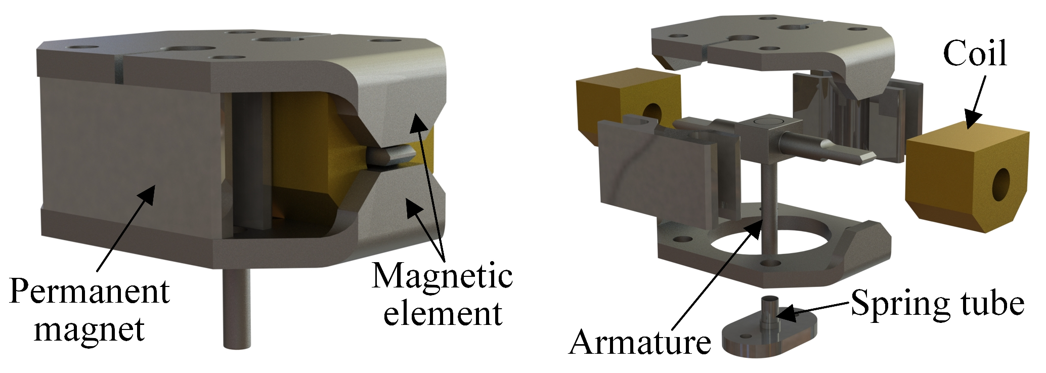
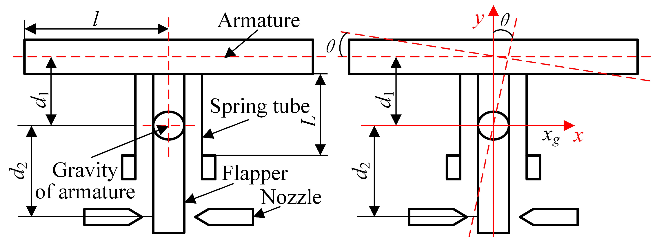
3.2. Armature Assembly Modeling

As shown in Figure 2, there is no equivalent sub-model in AMESim as a result of the cancellation of the feedback spring rod. The armature assembly model must be constructed in order to create the DREHSV simulation model.

The basic components of the armature assembly, as shown in Figure 5, are the armature, spring tube, and flapper [21]. The armature motion has two degrees of freedom (DOFs), deflection angle (θ) and horizontal displacement (x_g). The spring tube deforms while deflecting, causing horizontal movement (x_t). As a result, the matrix form can be used to express the torque tube (τ_tube) and spring tube force (F_tube).

$$\begin{array}{l}\left|\begin{array}{c}{F}_{tube}\\ {\tau }_{tube}\end{array}\right|=EI\left|\begin{array}{cc}12/L^3& -6/L^2\\ -6/L^2& 4/L\end{array}\right|\left|\begin{array}{c}{x}_t\\ \theta \end{array}\right|\\ x_t=x_g+d_1\theta \end{array}$$

(6)

where E is the Young’s modulus of the spring tube, I, is the inertia moment of the spring tube, L is the length of the spring tube, and d₁ is the distance between the armature center and the bottom of the spring tube.

The hydrodynamic force of the left and right nozzles applied to the flapper is calculated as follows:

$$F_L=f_l-f_r$$

(7)

where F_L is the resultant hydraulic force on the flapper, f_l is the hydraulic force on the left of the flapper, and f_r is the hydraulic force on the right of the flapper.

The equations of the armature motion are shown as follows:

$$\begin{array}{cc}\hfill J\ddot{\theta }& =T_d-b_r\dot{\theta }-{\tau }_{tube}+F_L{d}_2\hfill \\ & =T_d-b_r\dot{\theta }-EI\left(4\theta L-6x_g-6d_1\theta \right)/L^2+F_L{d}_2\hfill \\ \hfill m{\ddot{x}}_g& =-b_t{\dot{x}}_g-F_{tube}+F_L\hfill \\ & =-b_t{\dot{x}}_g-EI\left(12x_g+12d_1\theta -6\theta L\right)/L^3+F_L\hfill \end{array}$$

(8)

where J is the moment inertia of the armature, T_d is the electromagnetic torque, b_r is the rotational damping, d₂ is the distance between the armature center and the nozzle, m is the armature mass, and b_t is the moving damping.

The state equation of the armature is expressed by the matrix as follows:

$$\left|\begin{array}{c}\dot{\omega }\\ {\dot{v}}_g\\ \dot{\theta }\\ {\dot{x}}_g\end{array}\right|=\left|\begin{array}{cccc}\frac{-b_r}{J}& 0& \frac{-4EI/L+6EI{d}_1/L^2}{J}& \frac{6EI/L^2}{J}\\ 0& \frac{-b_t}{m}& \frac{6EI/L^2-12EI{d}_1/L^3}{m}& \frac{-12EI/L^3}{m}\\ 1& 0& 0& 0\\ 0& 1& 0& 0\end{array}\right|\left|\begin{array}{c}\omega \\ v_g\\ \theta \\ x_g\end{array}\right|+\left|\begin{array}{c}{T}_d+\left(f_r-f_l\right)d_2\\ f_l-f_r\\ 0\\ 0\end{array}\right|$$

(9)

Based on the theoretical analysis of the armature, the six-port armature component was constructed by using AMESet in AMESim, as shown in Figure 6.

First, three external variables were introduced to each port of the six-port armature. Second, the internal variables and actual parameters were set in the Type bar in AMESet. Finally, C code was assembled to produce the armature model in accordance with the theoretical analysis. In AMESim, the primary armature parameters are adjusted in accordance with

Table 2. Parameters of Armature.

Parameter	Value	Parameter	Value
m	0.0048 kg	d1	2.8 mm
J	5.3 × 10−7 kg·m2	d2	12.8 mm
L	4.5 mm	br	0.001 Nm/(rad/s)
E	1.2 × 106 bar	bt	100 N/(m/s)

.

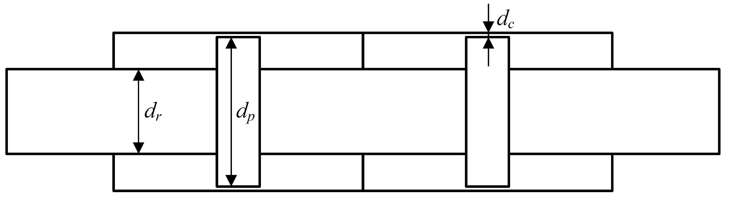
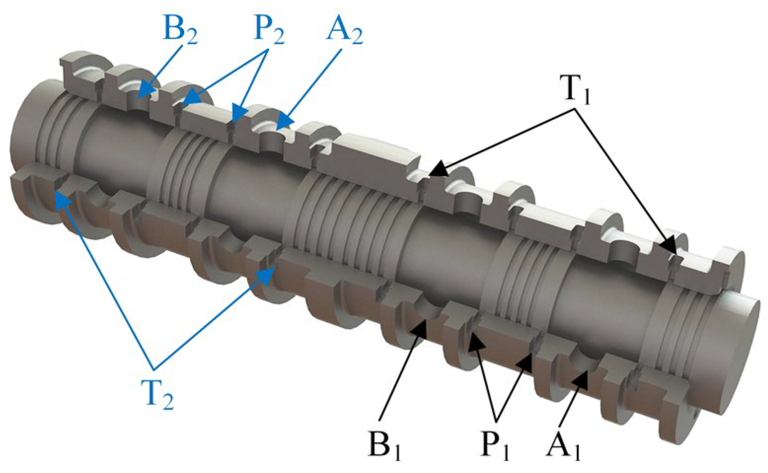
3.3. Double-System Slide Valve Modeling

The power stage spool of the standard servo valve was a four-sided slide valve, and the pilot stage differential pressure was supplied to both sides of the spool to cause it to move. In contrast to the common servo valve, the double system was used in the power stage of the DREHSV, as seen in Figure 7. In theory, the central main spool can be thought of as being made up of two spools of four-side sliding valves.

The force applied to the spool includes the driving force generated by the pilot stage, the inherent inertia force of the double-system spool and four pistons, the friction between the spool and valve sleeve, the steady fluid power, and external load force.

The pilot-stage driving force F_Q applied to the spool is shown as follows:

$$F_Q=4A_P{P}_L$$

(10)

where A_P is the force area of the piston and P_L is the pilot stage differential pressure.

When the spool and pistons move, the inertial force F_r is shown as follows:

$$F_r=m_v\frac{{\mathrm{d}}^2{x}_v}{\mathrm{d}{t}^2}$$

(11)

where x_v is the spool displacement and m_v is the total mass of the spool and four pistons.

The damping force F_m between the spool and valve sleeve and the piston and bush is shown as follows:

$$F_m=(B_v{}_1+B_{v2})\frac{\mathrm{d}{x}_v}{\mathrm{d}t}$$

(12)

where B_v1 is the damping coefficient between the spool and valve sleeve, and B_v2 is that between the piston and push.

The transient hydrodynamic force F_t is shown as follows:

$$F_t=B_f\frac{\mathrm{d}{x}_v}{\mathrm{d}t}$$

(13)

where B_f is the transient hydrodynamic force damping coefficient.

According to the Bernoulli equation, the jet velocity v at the slide valve port can be calculated as follows:

$$v=C_v\sqrt{\frac{2}{\rho }\Delta P}$$

(14)

where C_v is the velocity coefficient, ρ is the hydraulic oil density, and ΔP is the valve port differential pressure.

The flow area A_R of the double-system valve port is shown as follows:

$$A_R=4L_R{x}_v$$

(15)

where L_R is the rectangular valve port length.

The flow Q_L through the double-system valve port is shown as follows:

$$Q_L=C_d{A}_R\sqrt{\frac{2}{\rho }\Delta P}$$

(16)

where: C_d is the flow coefficient and C_d = 0.707.

The steady hydrodynamic force F_s can be calculated as follows:

$$F_s=2C_v{C}_{d}4L_R{x}_v\Delta P\cos \theta =K_f{x}_v$$

(17)

where θ is the ejection angle, K_f is the steady hydrodynamic force stiffness, and K_f = 8C_vC_d L_RΔPcosθ.

In summary, assuming that the external load force is F_L, the force balance equation of the double-system spool is shown as follows:

$$4A_P{P}_L={\mathrm{m}}_v\frac{{\mathrm{d}}^2{x}_v}{\mathrm{d}{t}^2}+(B_v{}_1+B_v{}_2+B_f)\frac{\mathrm{d}{x}_v}{\mathrm{d}t}+K_f{x}_v+F_L$$

(18)

According to Figure 7, four rectangular ports serve as the oil input and return ports, and four circular ports serve as the load ports. These ports are evenly spaced around the circumference. Therefore, the spool and valve sleeve were created by using the “BAO0003” sub-model with the specific throttling hole, as shown in Figure 8. It is assumed to have rounded edges, and there is a clearance between the spool and the valve sleeve. The pressure at port 2 was assumed to act on an active area adjacent to the orifice and tends to open the orifice, and the pressure at port 1 did not act directly on the spool. The net force is the sum of the pressure force and the external force. The velocity and displacement were input at port 3 and passed without modification to port 4. When the valve was nearly closed, the flow was assumed to be laminar. The key parameters of “BAO0003” are listed in

Table 3. Parameters of BAO0003.

Parameter	Value	Parameter	Value
Spool diameter	14.18 mm	Critical flow number	100
Rod diameter	11.3 mm	Underlap corresponding to zero displacement	0.008 mm
Width of a slot	1.95 mm	Rounded corner radius	0.007 mm
Depth of a slot	0.87 mm	Clearance on diameter	0.006 mm

.

The piston was used to transfer the pilot-stage differential pressure to drive the spool. The piston and bush were modeled using the “BAO043” sub-model, as shown in Figure 8.

The spool diameter of the piston was set to 17.02 mm, the rod diameter is set to 14.93 mm, and the force area of the piston (A_P) was calculated as $\frac{\pi }{4}\times \left({17.02}^2-{14.93}^2\right)=52.445{ \mathrm{mm}}^2$.

3.4. AMESim Overall Simulation Model

After modeling the key components of the pilot stage and power stage, the displacement sensor, PID controller, orifice, and other sub-models were added to construct the DREHSV simulation model [22], as shown in Figure 8.

According to Figure 8, the “MECMAS21” sub-model was used to represent the total mass of the spool and four pistons (m_v), and m_v was set to 0.6512 kg. The friction force is important during the movement of the spool, which can be modeled with a simple formulation taking into account Coulomb friction, stiction, viscous friction, and windage. In the DREHSV simulation model, the stiction force and Coulomb friction force were set at 10 N, and the coefficient of viscous friction was 2000 N/(m/s).

4. Simulation and Fault Research

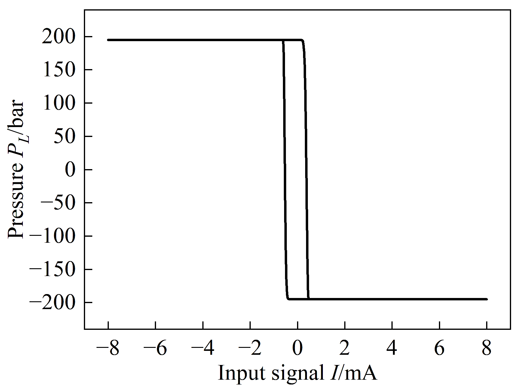
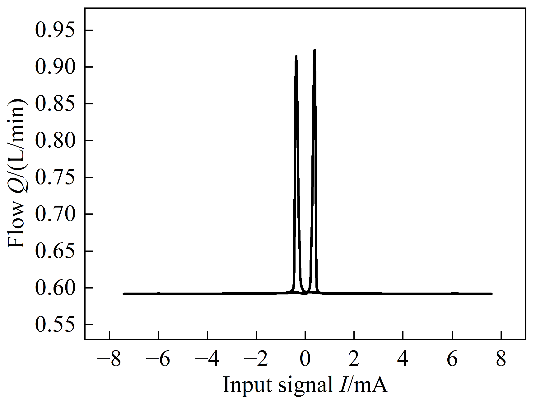
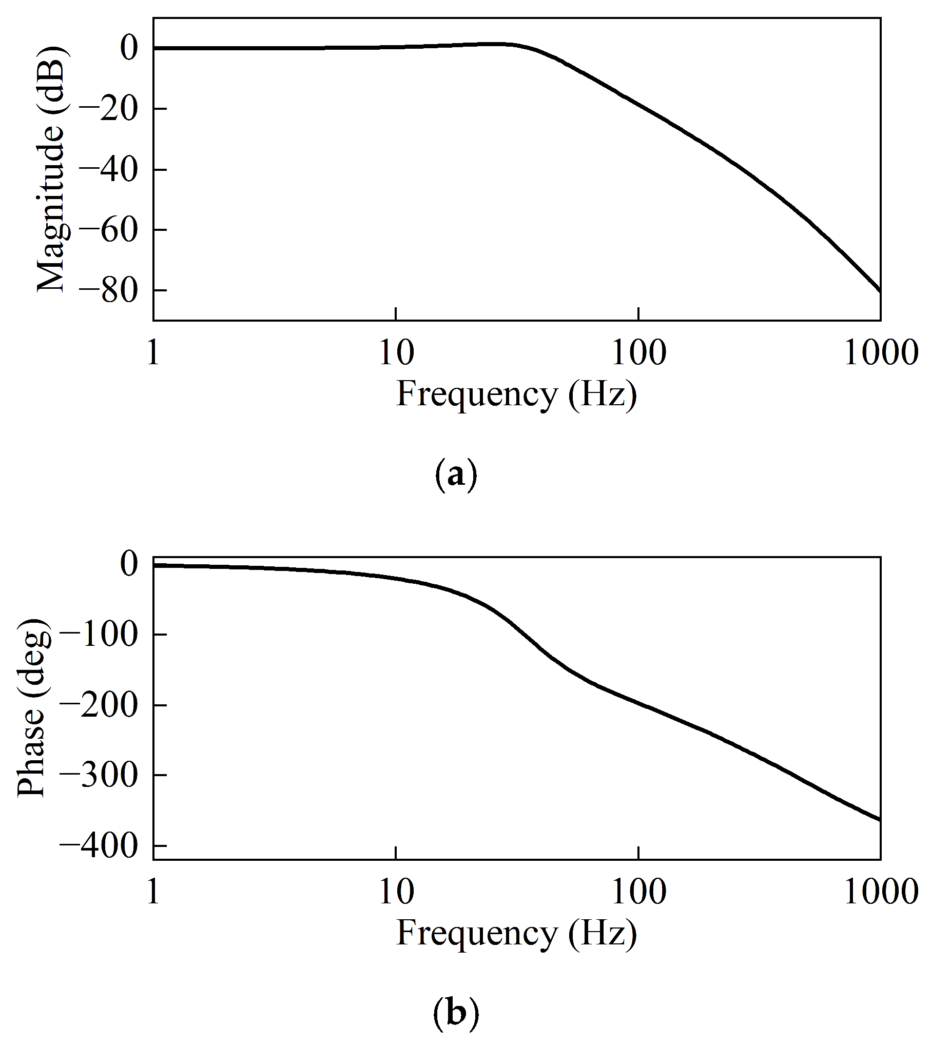
4.1. DREHSV Normal Mode

The control pressure is 11.5 MPa, while the supply pressure was set at 19.5 MPa. The sinusoidal input signal had a frequency of 1 Hz and an amplitude of 0.8. By using the model shown in Figure 8, the dynamic and static characteristics curves, which primarily contained pressure, no-load flow, and internal leakage characteristic curves, were derived, as illustrated in Figure 9, Figure 10 and Figure 11. It was sufficient to examine one system because the dynamic and static properties of the two systems were identical because the double-system parameters in the simulation model were the same.

Figure 9. Pressure Characteristic Curve.

Figure 9. Pressure Characteristic Curve.

When the actual output flow was zero, the relationship between the load pressure drop and the input signal was referred to as the “pressure characteristic curve”, which had a direct impact on the system’s bearing capacity and stiffness coefficient. The pressure gain, as shown in Figure 9, was 1659.36 bar/mA.

Figure 10. No-load Flow Characteristic Curve.

Figure 10. No-load Flow Characteristic Curve.

The relationship between the input signal and the output flow at the load port throughout the duration of an entire working cycle with no load pressure drop is known as the no-load flow characteristic curve. The flow gain, as shown in Figure 10, was 4.253 L/min/mA.

Figure 11. Internal Leakage Characteristic Curve.

Figure 11. Internal Leakage Characteristic Curve.

The internal leakage characteristic curve refers to the relationship between the oil return port flow and the input signal when the output flow is zero, which can measure the processing quality of the servo valve and the wear during service. According to Figure 11, the pilot stage leakage is 0.592 L/min, and the power stage leakage is 0.935 L/min.

The DREHSV is a closed-loop control system that relies on the displacement sensor at the right of the spool. Its response to a sine or step signal [23] can be utilized to evaluate its dynamic characteristics. To obtain the dynamic characteristic curves, the spool displacement was taken as the observed quantity, and the input signal was taken as the control quantity, as shown in Figure 12.

The phase bandwidth is 31.386 Hz and the amplitude bandwidth is 39.835 Hz, respectively, as shown in Figure 14. The precision and stability of closed-loop control can be seen in the dynamic and static characteristic curves.

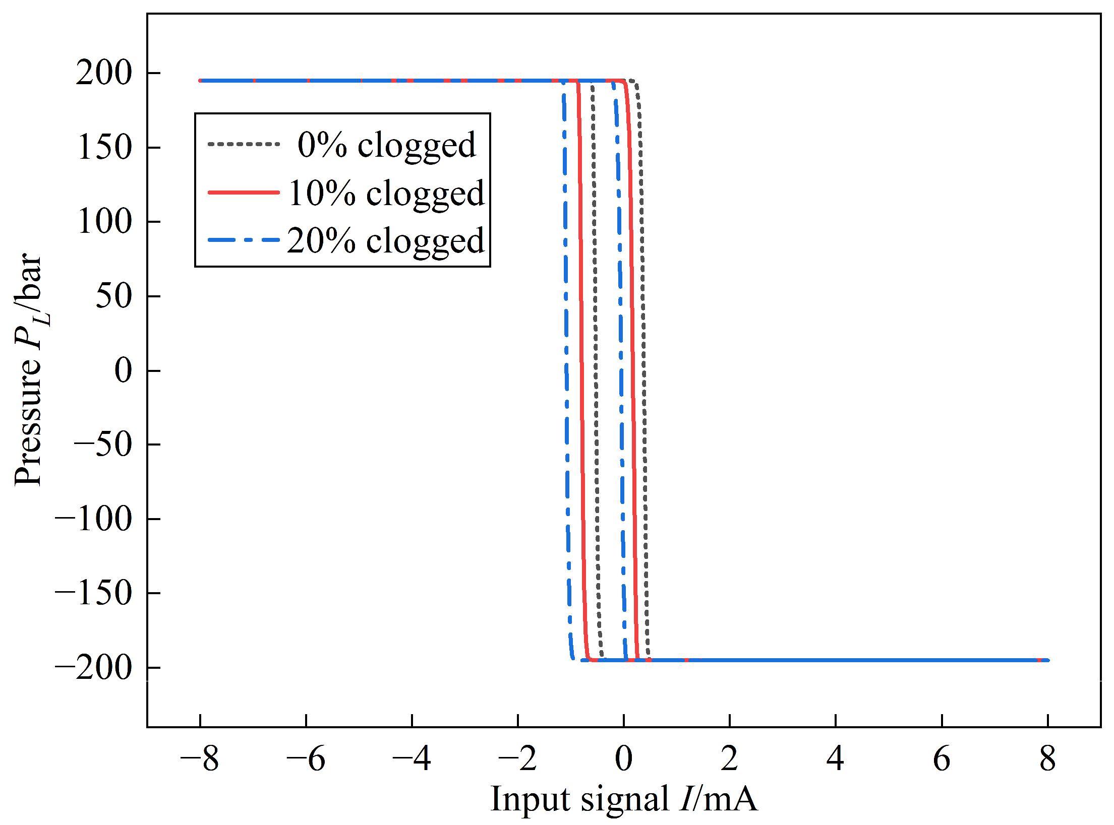
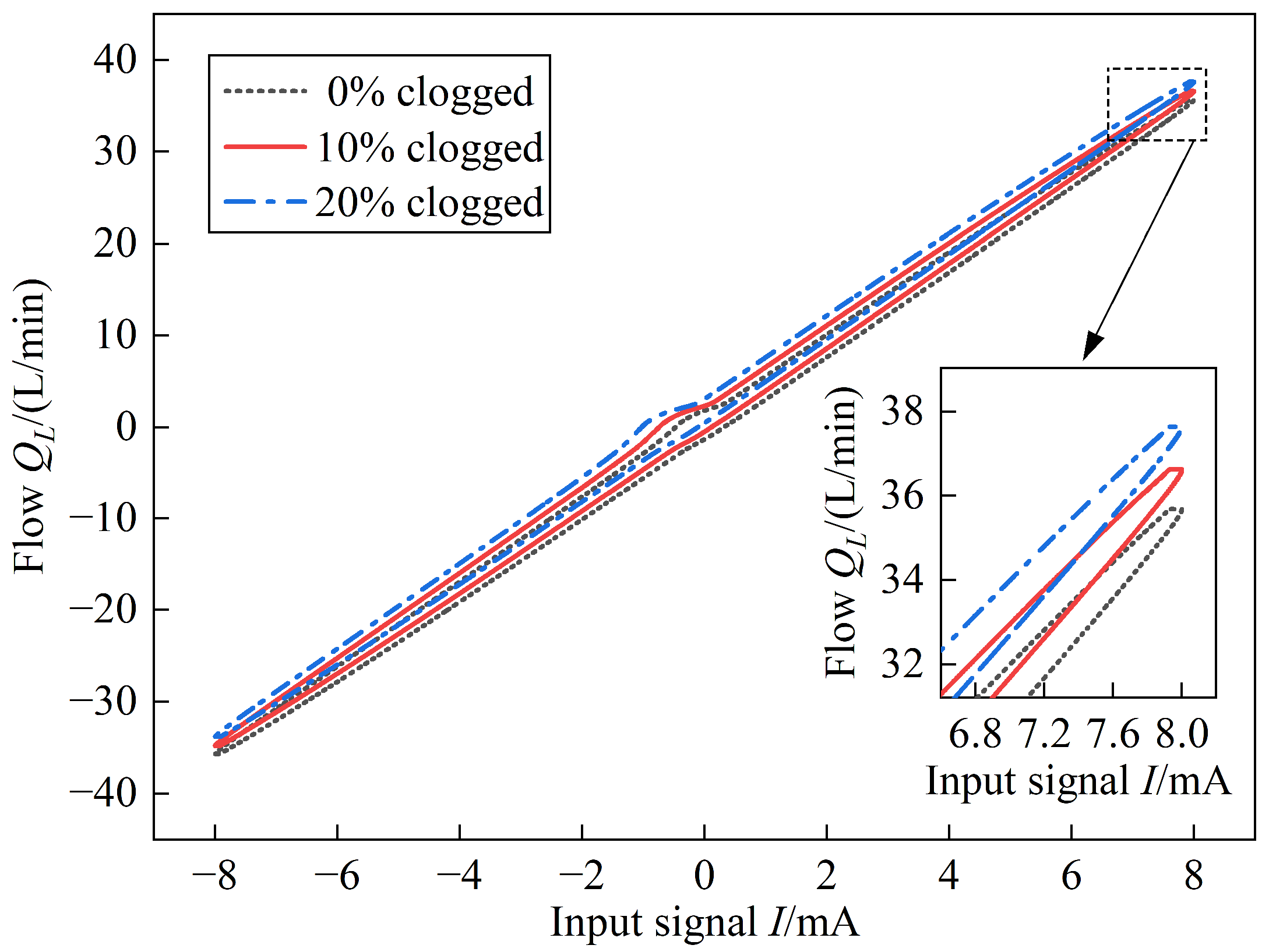
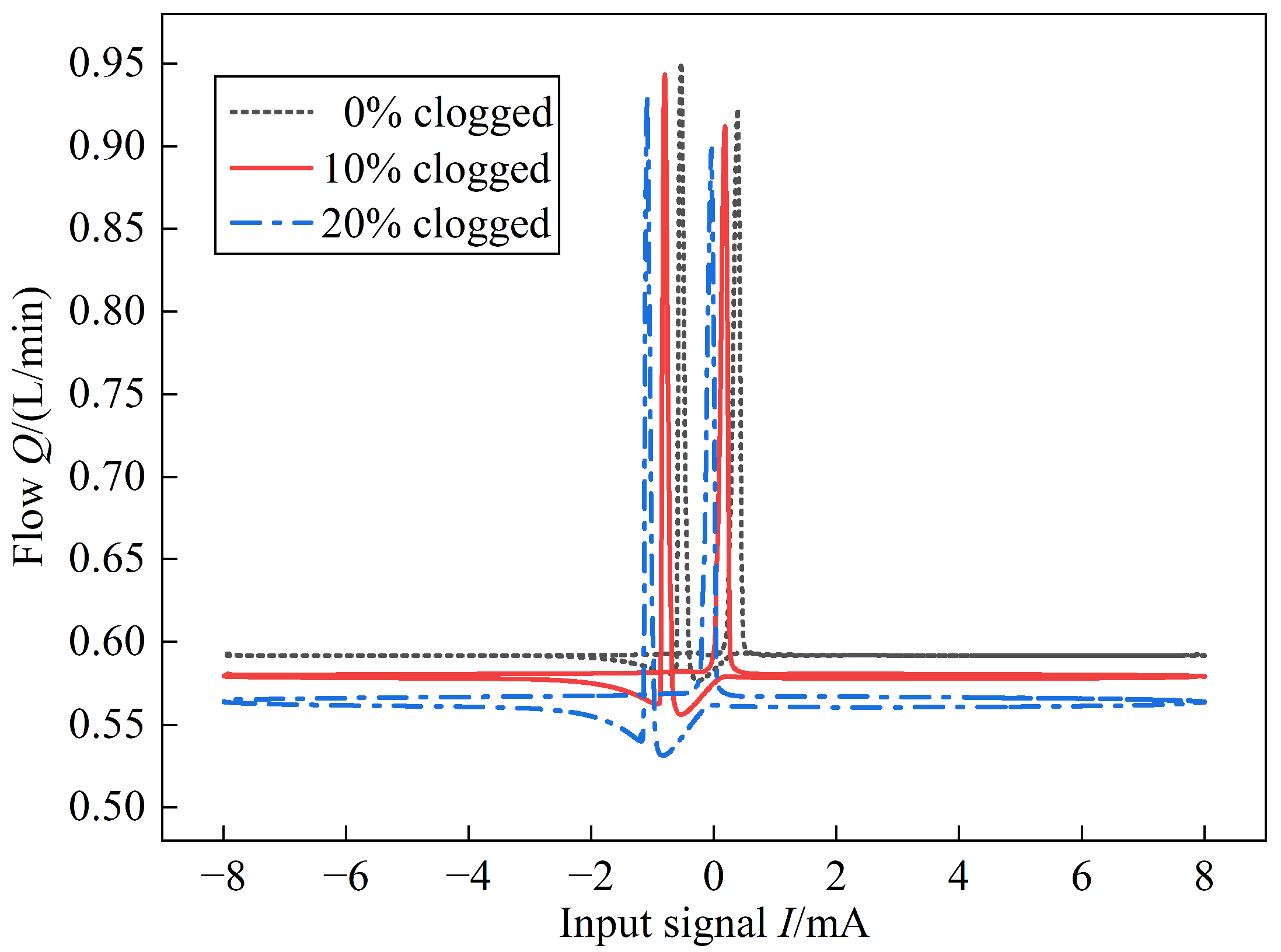
4.2. Pilot Stage Nozzle Clogged

In the process of long-term service, the nozzle was easily clogged by impurities and particles in the oil. In addition, there was rust and wear inside the nozzle [24], affecting its patency and causing the nozzle to be clogged.

The static characteristic curves are obtained when the clogging degree was 10% and 20% by altering the left nozzle size to simulate various clogging degrees, as shown in Figure 13, Figure 14 and Figure 15.

According to Figure 13 and Figure 14, the pressure and flow characteristic curves shift to the left as the clogging degree of left nozzle rises; the higher the clogging degree, the higher the zero-bias value, but the pressure and flow gain stay constant. According to Figure 15, the internal leakage characteristic curve shifts to the left, and the leakage decreases with the increase in clogging degree.

The degree of clogging in nozzle results in a decrease in nozzle size, an increase in the throttling effect, and a reduction in the flow through the nozzle. The differential pressure becomes larger, resulting in a pressure change in the control cavity, which changes the static characteristic.

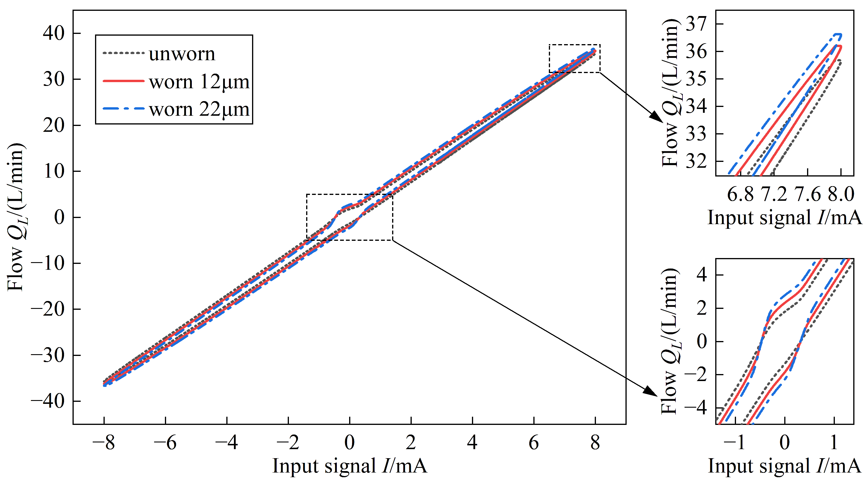
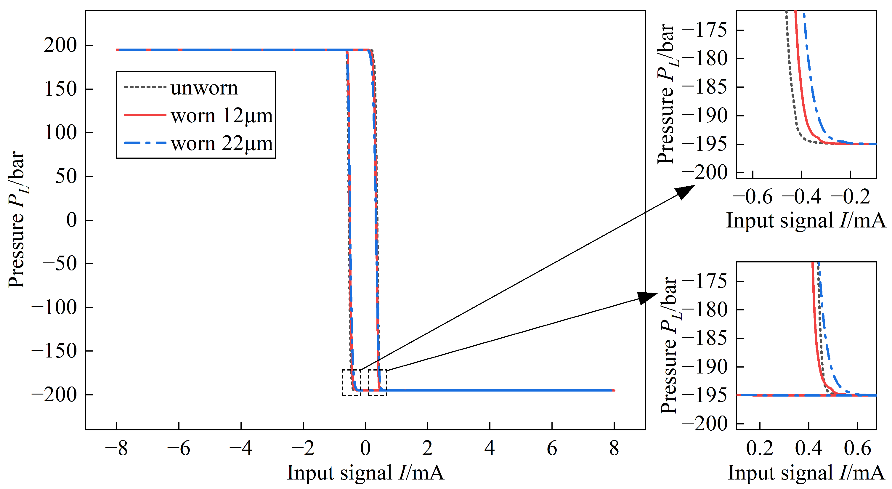
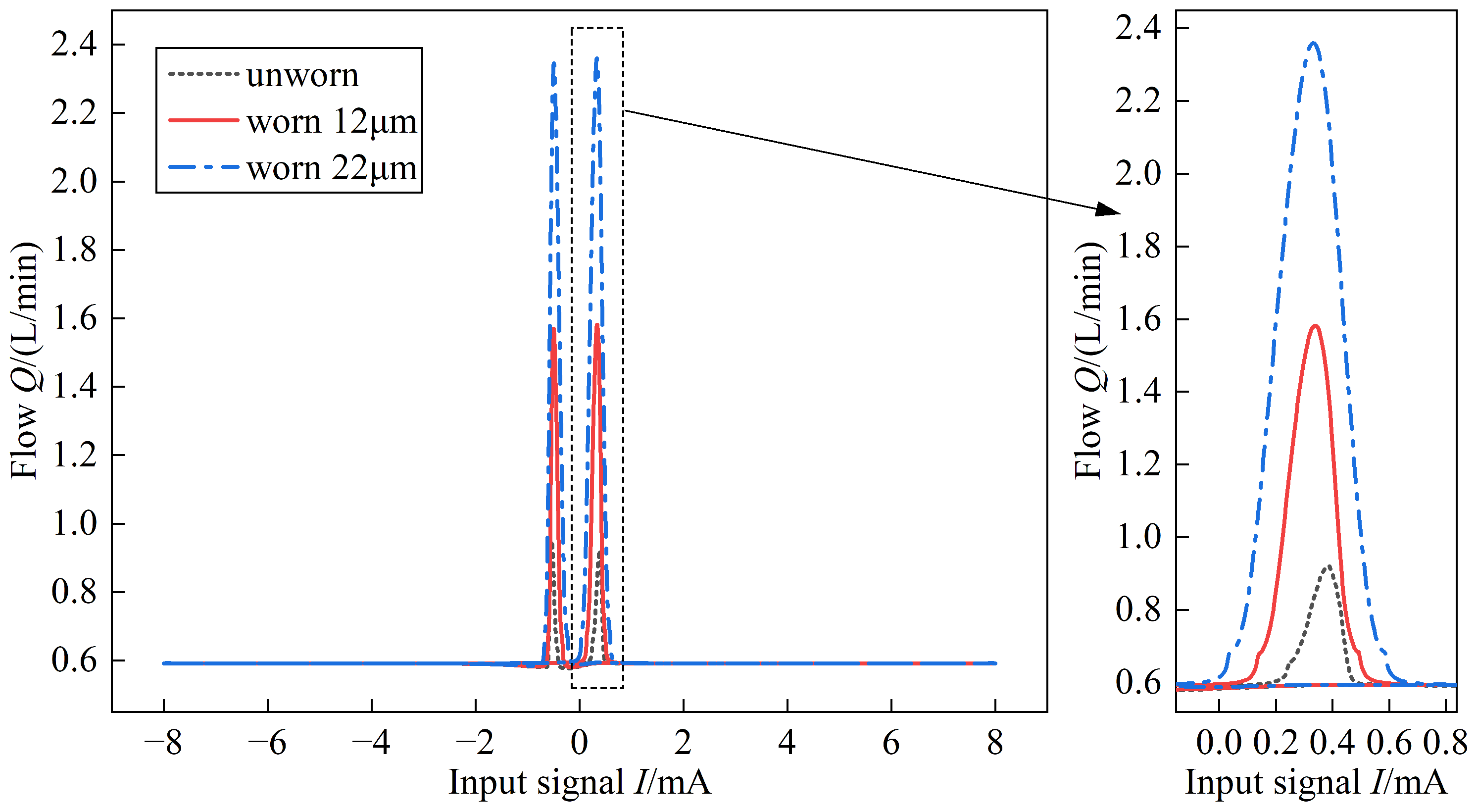
4.3. Power Stage Spool Worn

The DREHSV was in a high-load state for a long time, and the spool was subjected to greater pressure and impact, resulting in the wear of the spool throttling edge. In addition, under pressure action, the spool throttling edge was also impacted by the impurities in the oil, which further aggravates the wear of the spool.

Because the wear of the throttling edge of the spool caused the opening of the spool to increase, the wear of the spool can be simulated by gradually changing the opening of the spool in the simulation model. The static characteristic curves of the spool throttling edge worn at 12 μm and 22 μm were obtained by setting two different opening values of the opening to12 μm and 22 μm, as shown in Figure 16, Figure 17 and Figure 18.

As the worn degree increases, according to Figure 16, the pressure gain near the zero position decreases. According to Figure 17, the flow gain near the zero position increases, and the curve peak value also increases. According to Figure 18, the leakage at the zero-position increases sharply, but the pilot stage leakage does not change significantly.

The tiny gap between the spool and the valve sleeve became larger because of the wear of the spool throttling edge, which resulted in unstable movement in the spool and reduced the control accuracy. The spool wear also led to a decrease in the sealing between the spool and valve sleeve, which made the leakage near the zero position increase sharply.

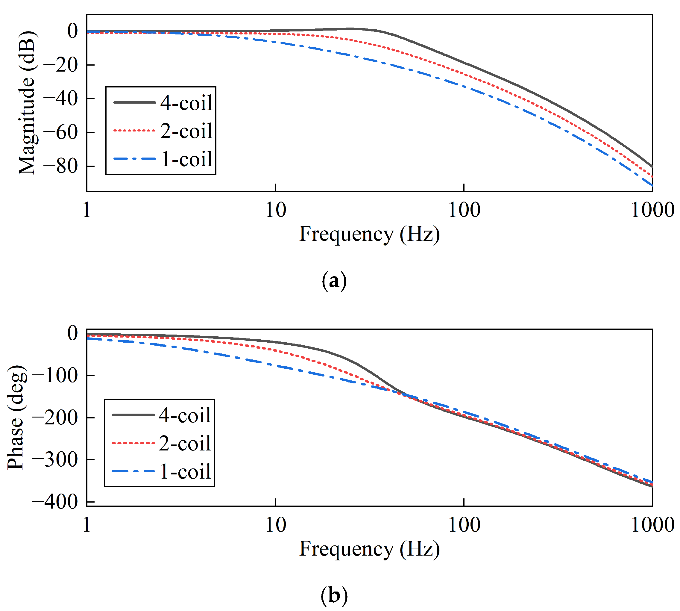
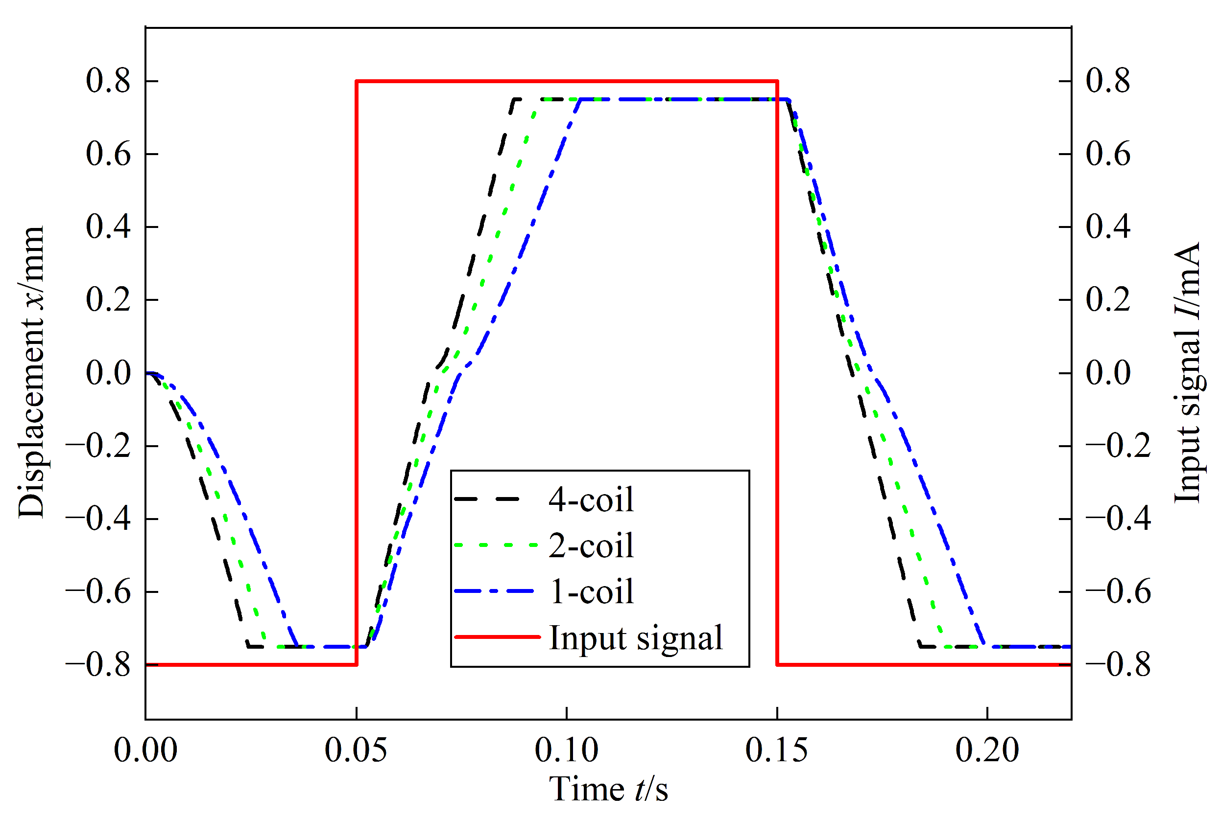
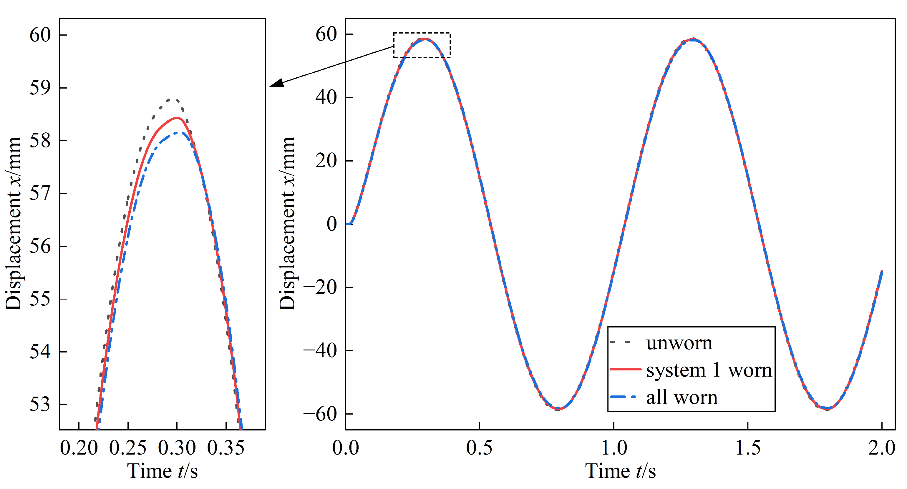
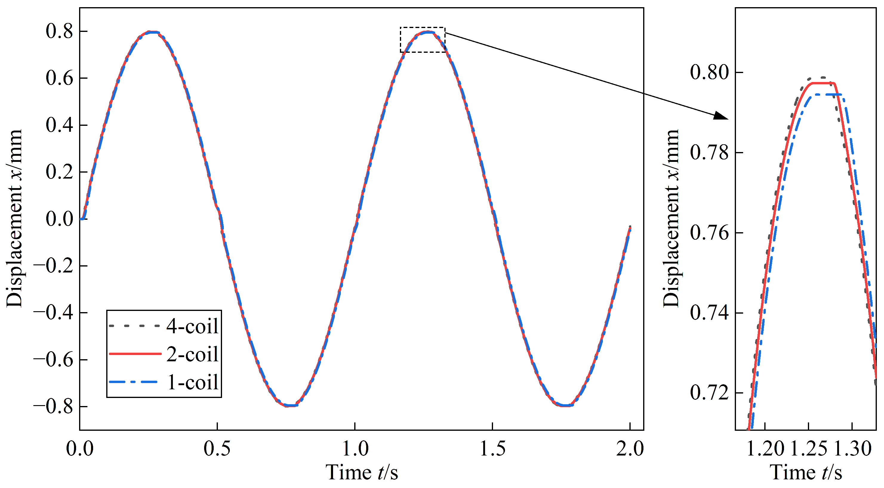
4.4. Redundant Design Advantage

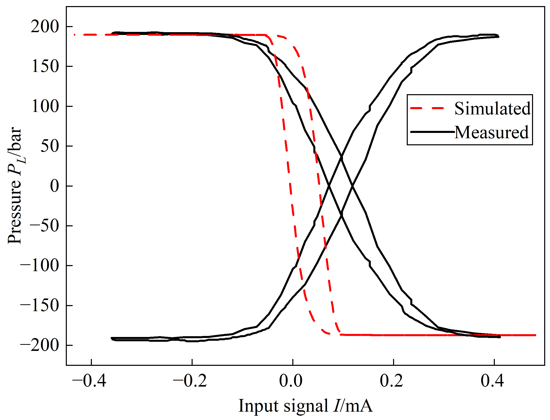
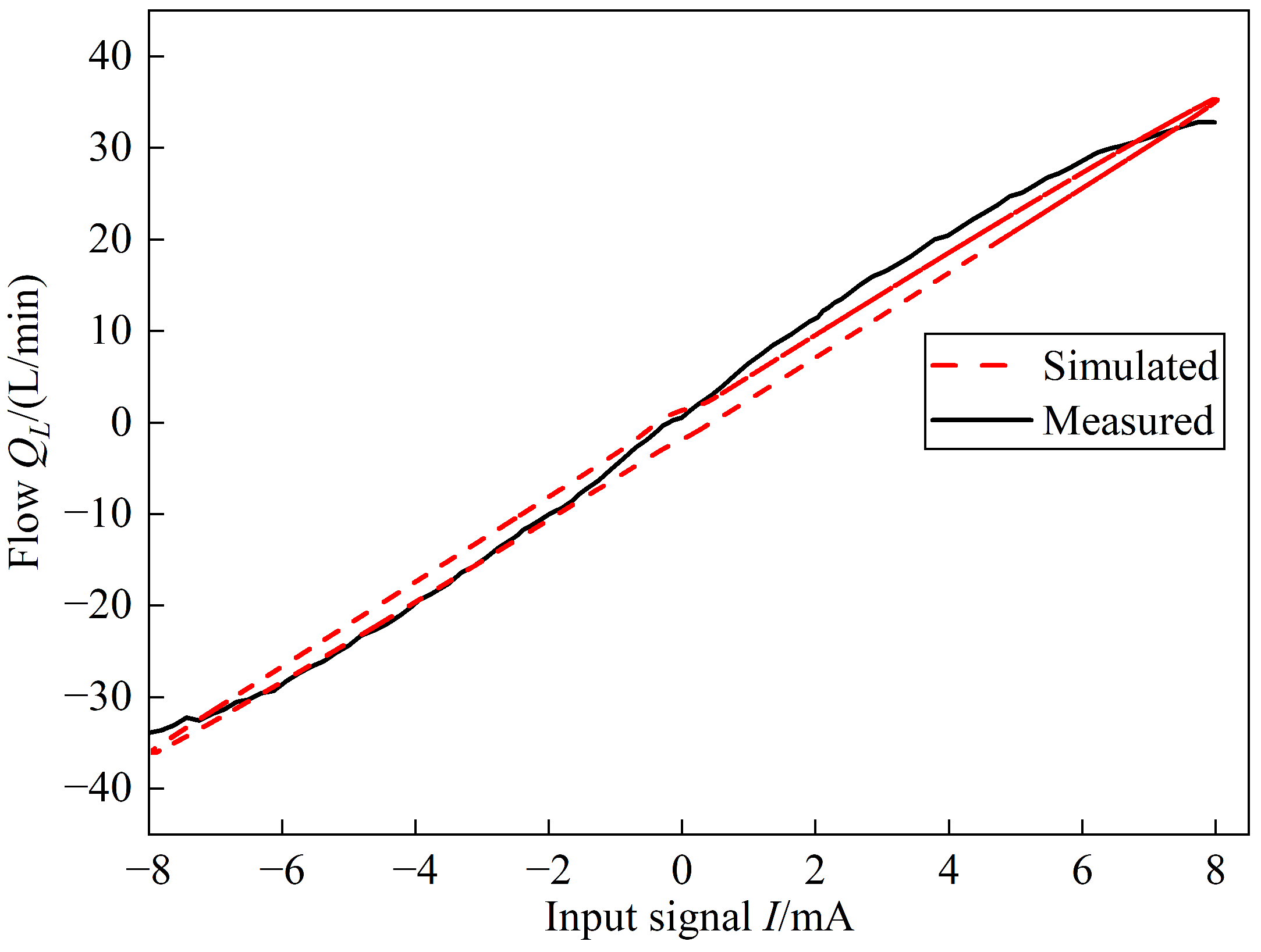
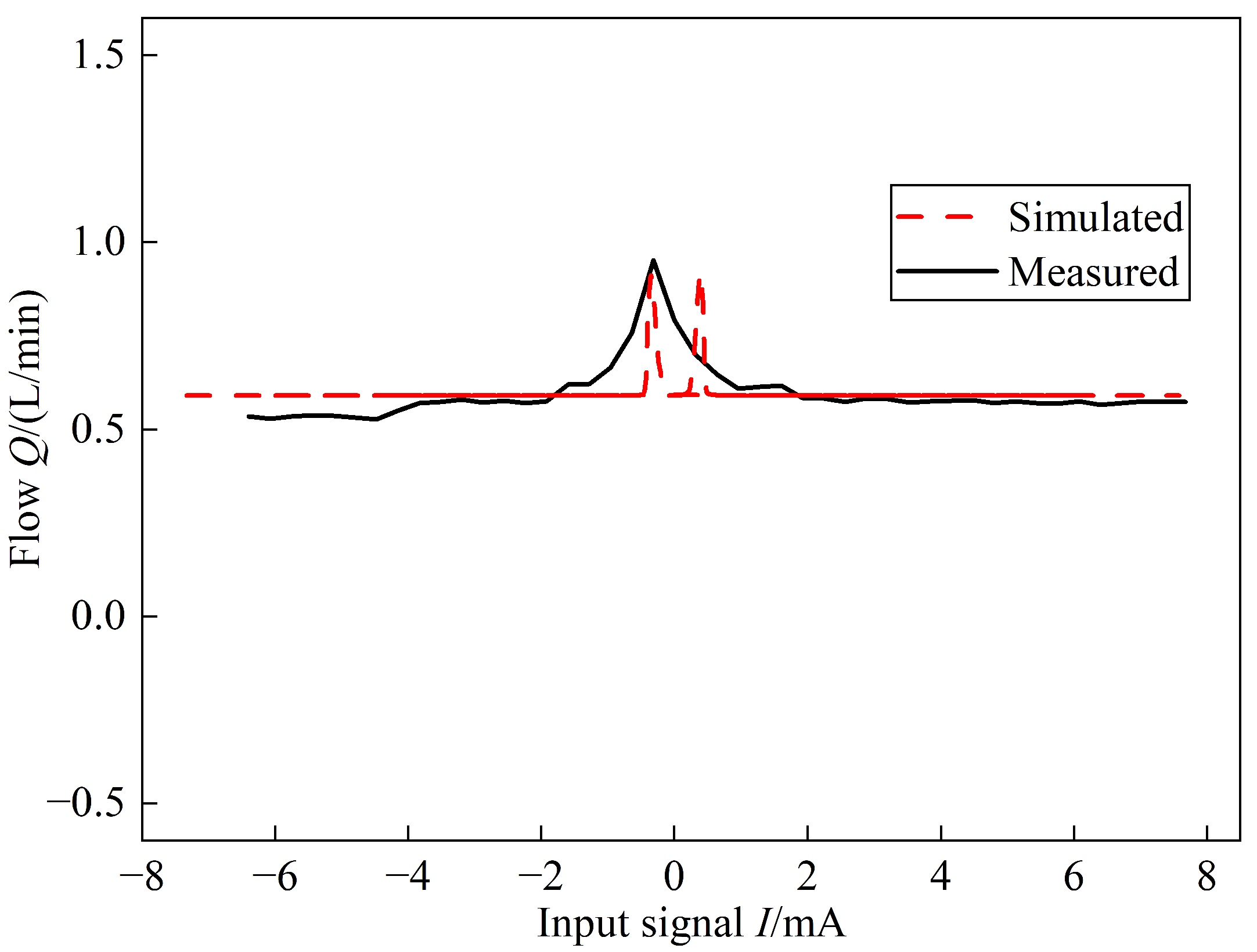
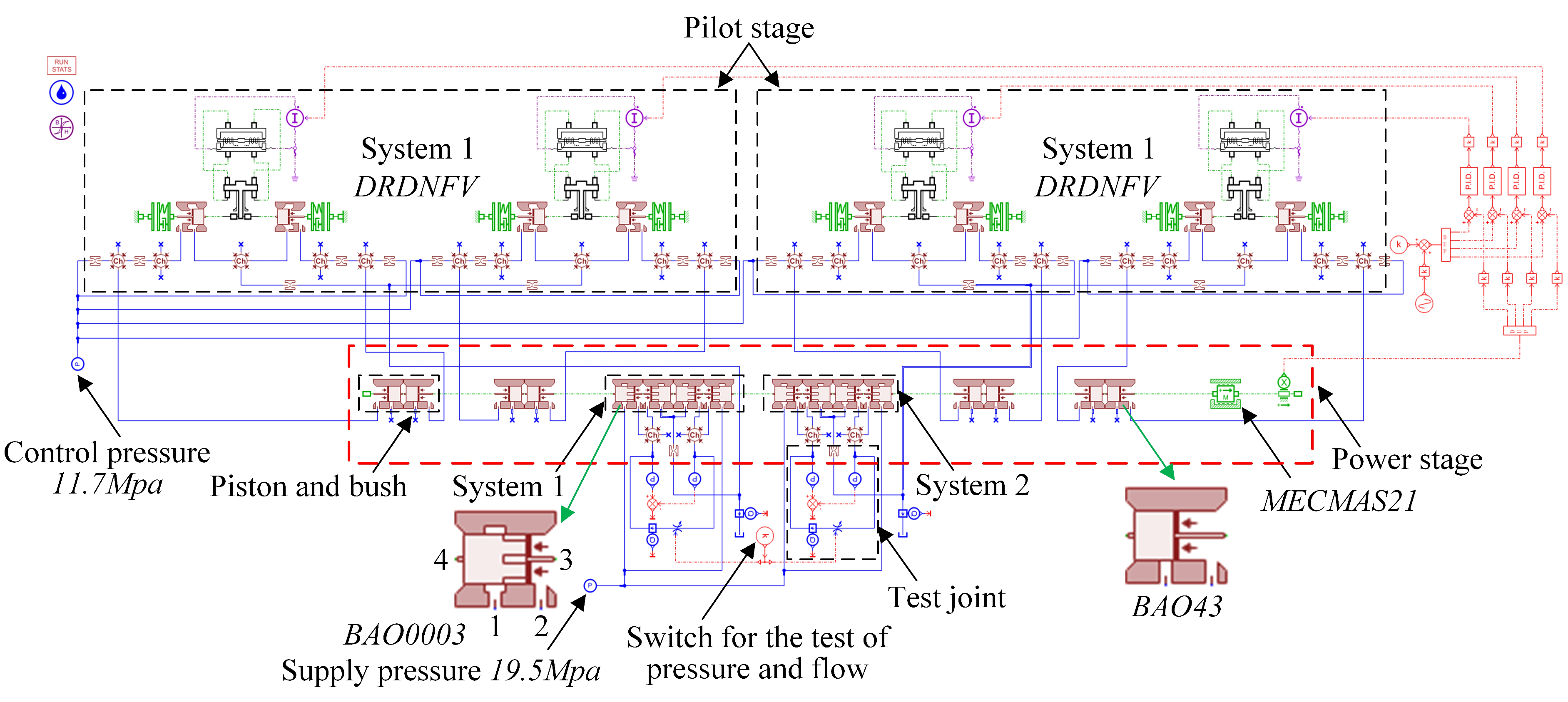
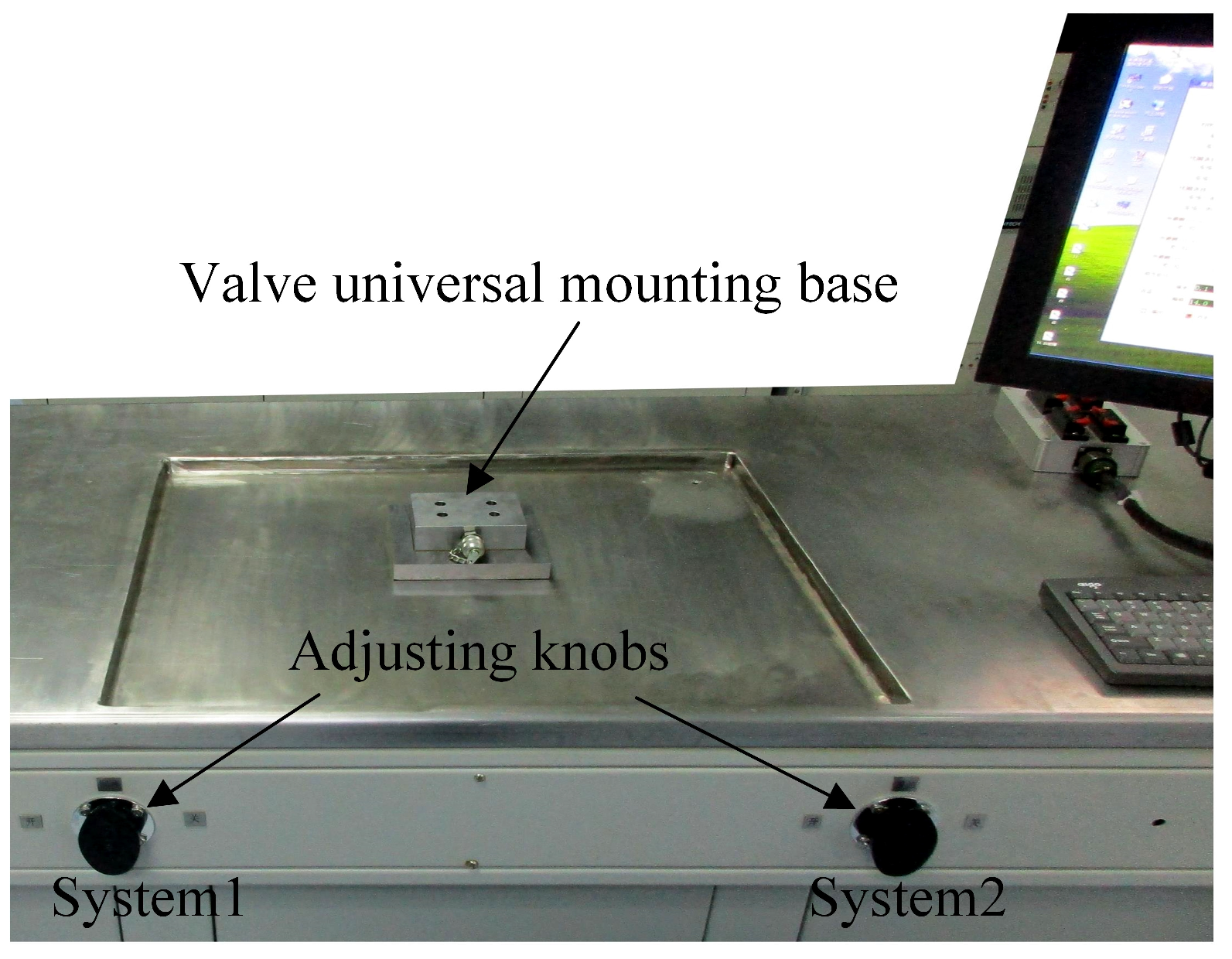
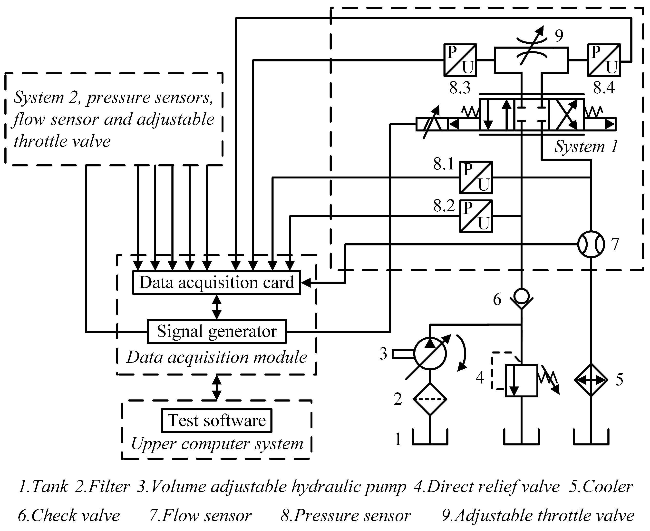
The electrical four-redundancy design was adopted in the DREHSV pilot stage, and the double-system slide valve of the power stage was divided into two systems. Each system can be considered a four-side slide valve. It was essential to assess the advantages of the redundant design independently for the pilot stage and power stage because they are both redundant.

The redundancy advantage of the pilot stage was reflected in the control of the spool displacement in the power stage. In normal mode, four identical feedback signals from the four-coil displacement sensor were input into the four torque motors. To demonstrate the benefit of the redundant pilot stage design, the performance of the DREHSV under the pilot stage differential pressure was simulated in AMESim by disconnecting the coil signal.

According to Figure 19, the dynamic response slows down with the decrease in the number of working coils, because there was no signal input to the torque motor connected with the cut coil. The torque motor floated without electromagnetic torque output, and the total driving force applied to the spool decreased. The amplitude and phase bandwidth are shown in

Table 4. Amplitude and Phase Bandwidth.

Number of Coils	Amplitude	Phase
4	39.835 Hz	31.386 Hz
2	17.983 Hz	22.931 Hz
1	5.497 Hz	14.871 Hz

.

The dynamic response was greatly affected by the number of pilot-stage working coils. When the coil signal was cut off in the common EHSV, the servo valve was unable to work any more. However, due to the use of a redundant design in the pilot stage, as long as one coil continues to work, the pilot stage remained capable of producing the driving force required to drive the spool movement of the power stage, and the spool could still reach the predetermined position required to ensure the maximum output of pressure and flow, although the response time is slower. The spool displacement curve under the action of the sinusoidal signal [25] is shown in Figure 20.

Under various coil counts, the maximum displacement that the spool can achieve and the required time are shown in

Table 5. Maximum Displacement and Required Time of the Spool.

Number of Coils	Maximum Displacement	Required Time
4	0.798 mm	0.271 s
2	0.797 mm	0.278 s
1	0.794 mm	0.286 s

.

The theoretical maximum displacement of the power stage spool is 0.8 mm. According to Table 5, when the valve was in the normal mode of the four coils, the maximum displacement that the spool could achieve was 0.798 mm and the control accuracy was 1 − (0.8 − 0.798)/0.8 = 99.75%. When the two coils were working, the maximum displacement was 0.797 mm, and the control accuracy was 1 − (0.8 − 0.797)/0.8 = 99.625%. When only one coil was working, the maximum displacement was 0.794 mm, and the control accuracy was 1 − (0.8 − 0.794)/0.8 = 99.25%.

In AMESim, the input signal was changed to the step signal, and the spool displacement response curves for the different numbers of coils were obtained, as shown in Figure 21.

According to Figure 21, the spool displacement nearly corresponds with the input signal when the coil signal is not cut off, and the delay time of the first stage is 0.0245 s, which shows the excellent dynamic characteristics of the DREHSV [26]. When the signals from two coils were cut off, the delay time was 0.0290 s. When the signal of only one coil was not cut, the delay time was 0.0362 s. As the number of working coils decreased, the followability became worse, but the spool was still able to reach the predetermined position, which had good fault tolerance. Therefore, the advantage of the redundant design of the pilot stage has been further proven.

This type of servo valve has been mainly used in a specific sort of canard wing actuator. The double-system hydraulic cylinder was powered by the DREHSV, and the hydraulic cylinder was connected with a canard wing to control the movement of the aircraft. The double-system hydraulic cylinder had two sets of oil inlet chambers and oil return chambers, in which each set of oil inlet chambers and oil return chambers were connected to the load port of the double-system slide valve. The piston diameter (d_p) was 62.8 mm, the rod diameter (d_r) was 38.7 mm, and the clearance on the diameter (d_c) was 0.03 mm, as shown in Figure 22.

The simulation model of the DREHSV-controlling double-system hydraulic cylinder is shown in Figure 23. The advantage of a redundant design for the power stage is mainly reflected by the double-system hydraulic cylinder. Power stage spool wear is a frequent cause of failure. To account for this, three working scenarios—“double system spool no wear”, “single system spool wear”, and “double system spool all wear”—were set in the simulation model. By comparing the displacement curves of the hydraulic cylinder under these three conditions, as shown in Figure 24, the benefits of the power stage redundant design are demonstrated.

The maximum displacement that the hydraulic cylinder can achieve and the required time under the situation of different spool wear parts are shown in

Table 6. Maximum Displacement and Required Time of The Actuator.

Different Wear Parts	Maximum Displacement	Time
Unworn	58.807 mm	0.296 s
System 1 worn	58.431 mm	0.300 s
All worn	58.156 mm	0.303 s

.

The theoretical maximum displacement of the hydraulic cylinder was 60 mm. According to Table 6, when the spool was unworn, the maximum displacement that the hydraulic cylinder can achieve was 58.807 mm, and the control accuracy was 1 − (60 − 58.807)/60 = 98.01%. When the spool of system 1 was worn at 22 μm, the maximum displacement was 58.431 mm, and the control accuracy is 1 − (60 − 58.431)/60 = 97.39%. When the spool of the double system was all worn, the maximum displacement was 58.156 mm, and the control accuracy was 1 − (60 − 58.156)/60 = 96.93%. The maximum displacement in the first cycle, as well as the time required to reach the maximum displacement, were within the allowed ranges. For double-system hydraulic cylinders, the power stage double-system slide valves perform reliably, guaranteeing that the hydraulic cylinders fulfill the required actions.

5. Experiment

The pressure, flow, internal leakage, and dynamic response test experiments of the DREHSV were carried out on a test bench. According to Figure 25, there was a universal valve mounting base, two adjusting knobs, and a PC controller on the test bench. As shown in Figure 26, the DREHSV test system included the upper computer system, data acquisition system, and hydraulic test system. The test system of the upper computer was divided into the test software, which realized the functions of dynamic and static characteristic testing, data storage and playback, and report generation. The data acquisition module included a data acquisition card and a signal generator. The signal generator sent the command signal sent by the data acquisition card or the command signal generated by itself to the torque motor and feedbacked the command signal and valve spool displacement to the data acquisition card. The data acquisition card collected the output flow, inlet pressure, outlet pressure, load port pressure, command signal, and spool displacement feedback of the hydraulic test system in the upper position machine. The main components of the hydraulic test system were the oil source and the test bench. The oil source provided the constant-pressure 10# aviation hydraulic oil for the test bench to ensure that the DREHSV can work normally. The test bench was equipped with a flow sensor and a pressure sensor to measure the system flow and the pressure at ports P, T, A, and B of the DREHSV. The test bench was also equipped with an adjustable throttle valve to simulate the valve load and different valve blocks to replicate the test of various characteristics of the valve. The tested DREHSV was mounted on the base via a transfer valve block. The adjusting knobs were responsible for controlling the oil supply of the two systems, respectively.

The dynamic and static characteristic curves were obtained as shown in Figure 27, Figure 28, Figure 29 and Figure 30.

Figure 27. Pressure Characteristic Curve (Test).

Figure 27. Pressure Characteristic Curve (Test).

Comparing Figure 9 and Figure 27, the test pressure gain is 1552.60 bar/mA, and the simulation error is calculated as (1659.36 − 1552.60)/1552.60 = 7.080%.

Figure 28. No-load Flow Characteristic Curve (Test).

Figure 28. No-load Flow Characteristic Curve (Test).

Comparing Figure 10 and Figure 28, the test flow gain is 4.715 L/min/mA, and the simulation error is calculated as (4.715 − 4.253)/4.715 = 9.780%.

Figure 29. Internal Leakage Characteristic Curve (Test).

Figure 29. Internal Leakage Characteristic Curve (Test).

Comparing Figure 11 and Figure 29, the test pilot stage leakage is 0.574 L/min, and the simulation error is calculated as (0.592 − 0.574)/0.574 = 3.136%. The test power stage leakage is 0.969 L/min, and the simulation error is (0.969 − 0.935)/0.969 = 3.509%.

Figure 30. Dynamic Characteristic Curve (Test).

Figure 30. Dynamic Characteristic Curve (Test).

Comparing Figure 12 and Figure 30, the test amplitude bandwidth is 33.456 Hz, and the simulation error is (39.835 − 33.456)/33.456 = 19.067%. The test phase bandwidth is 26.866 Hz, and the simulation error is (31.386 − 26.866)/26.866 = 16.824%.

The simulation results are basically consistent with the experimental test results, and the errors are all within the allowed range of quality inspection. The correctness of the simulation model is verified by the static and dynamic characteristic experiments.

6. Conclusions

(1) This paper suggests a modeling approach for the servo valve with a redundancy structure using AMESim. On the test bench, the dynamic and static characteristic curves were displayed and the general trend of the experimental curves agreed with the outcomes of the simulation. The fact that all of the errors fall within the acceptable range proves that the theoretical analysis and simulation model are accurate.

(2) The AMESim model was used to simulate the effects of typical faults, such as the degree of clogging in the nozzle and the degree of wear of the spool throttling edge, on the static characteristics. It was discovered that the zero bias value increases with the degree of clogging. With more blockage, there was less internal leakage. As the flow gain near zero increased, the zero leakage increases dramatically, and the pilot-stage leakage did not change significantly when the spool throttling edge wore. The accuracy of the simulation model was further confirmed through the simulation of common problems, and the model also had the ability to simulate other defects.

(3) The advantages of a redundant design were verified through the simulation. When the coil is cut off, the response will become slower, but the spool displacement does not change very much, and the spool can still reach the predetermined position. When the valve was in the normal mode of four coils, the control accuracy was 99.75%. When only one coil was working, the control accuracy was 99.25%, which had excellent fault tolerance and reliability in the pilot stage. For the power stage double-system slide valves, when the spool was unworn, the control accuracy was 98.01%. When the spool of the double system was all worn, the control accuracy was 96.93%. By introducing typical defects to the pilot and power stages, respectively, the simulation confirmed the advantage of adopting redundant designs for the pilot and power stages.

(4) The DREHSV simulation model was established using AMESim, and various operating states of the valve were simulated by changing the parameters of the model, which lay the foundation for later performance analysis and fault simulation. In addition, rich sample data, which can be used in the fault diagnosis of the DREHSV, can be generated by the model.

References

1. Fang, Q.; Huang, Z. Developing process, research actuality and trend of electrohydraulic servo valve. Mach. Tool Hydraul. 2007, 35, 162–165. [Google Scholar]
2. Ye, H.; Zeng, G.S. Structure design and reliability analysis of the triplex redundance digital servo control system. J. Solid Rocket. Technol. 2002, 25, 69–72. [Google Scholar]
3. Anderson, R.T.; Li, P.Y. Mathematical modeling of a two spools flow control servovalve using a pressure control pilot. J. Dyn. Syst. Meas. Control. 2002, 124, 420–427. [Google Scholar] [CrossRef]
4. Chen, Z.G.; Ding, F.; Cai, Y.H. Research on characteristics of single-stage twin flapper-nozzle electrohydraulic servo valve. Mach. Tool Hydraul. 2007, 35, 114–116, 135. [Google Scholar]
5. Mu, D.J.; Li, C.C.; Yan, H.; Sun, M. Nonlinear simulation and linearization of twin flapper-nozzle servo valve. J. Mech. Eng. 2012, 48, 193–198. [Google Scholar] [CrossRef]
6. Wang, D.W. Flow Field Characteristics Research and Malfunction Simulation Analyses on the Three-Stage Servo Valve. Ph.D. Thesis, Harbin Institute of Technology, Harbin, China, 2013. [Google Scholar]
7. Liu, C.H. Study on Modeling and Simulation of Two-Stage Nozzle-Flapper Servo Valve with Force Feedback. Ph.D. Thesis, Harbin Institute of Technology, Harbin, China, 2013. [Google Scholar]
8. Wang, X.Q.; Wang, W.F. Modeling and simulation of armature assembly of double-stage double-nozzle-flapper electro-hydraulic servo valve. Mach. Tool Hydraul. 2014, 42, 161–165, 199. [Google Scholar]
9. Gordic, D.; Babic, M.; Jovicic, N. Modelling of spool position feedback servo valves. Int. J. Fluid Power 2014, 5, 37–50. [Google Scholar] [CrossRef]
10. Gordic, D.; Babic, M.; Milovanovic, D.M. Effects of the variation of torque motor parameters on servo valve performance. Stroj. Vestn. J. Mech. Eng. 2008, 54, 866–873. [Google Scholar]
11. Li, L.F.; Yu, M.H.; Ma, C.F.; Guo, X.; Dong, M. Simulation and fault research for two stage double nozzle flapper electro-hydraulic servo valve based on AMESim. Mach. Tool Hydraul. 2017, 45, 177–180. [Google Scholar]
12. Li, Y.S. Physical model of two-stage nozzle-flapper electrohydraulic servo-valve with force feedback. Chin. Hydraul. Pneum. 2021, 45, 69–73. [Google Scholar]
13. Shi, S.M. The Fault Diagnosis of the Electro-Hydraulic Servo Valve Based on Neural Network. Ph.D. Thesis, Yanshan University, Qinhuangdao, China, 2022. [Google Scholar]
14. Yan, H.; Yao, L.; Qiu, L.; Yan, H. Modelling and fault tolerance analysis of triplex redundancy servo valve. Int. J. Model. Identif. Control 2019, 31, 27–38. [Google Scholar] [CrossRef]
15. Chen, K.Q.; Zhao, S.J.; Liu, H.X. The study on the high power redundant electro-hydraulic actuator for launch vehicles. Missiles Space Veh. 2020, 6, 79–84+122. [Google Scholar]
16. Han, T.Y.; Im, D.S.; Hahn, B. Force-fighting phenomena and disturbance rejection in aircraft dual-redundant electro-mechanical actuation systems. Actuators 2023, 12, 310–328. [Google Scholar] [CrossRef]
17. Yan, P.Y. Design of Industrial Two-Dimensional (2D) Servo Valve and Its Double Redundant Controller. Ph.D. Thesis, Zhejiang University of Technology, Hangzhou, China, 2020. [Google Scholar]
18. Qin, J.Y.; Li, C.C.; Yan, H. Effect of temperature on torque motor air gap reluctance and permanent magnet polarization magnetomotive force. Mach. Tool Hydraul. 2017, 45, 105–109. [Google Scholar]
19. Yin, Y.B.; Guo, W.K.; Li, R.H. Magnetic circuit modeling and characteristic analysis of torque motor considering magnetic leakage. J. Harbin Eng. Univ. 2020, 41, 1840–1846. [Google Scholar]
20. Huang, C.C.; Yan, C.K.; Zhang, J.N.; Xu, D.F.; Jin, Z. Analysis of influencing factors of servo torque motor output torque. Chin. Hydraul. Pneum. 2021, 45, 65–70. [Google Scholar]
21. Kang, J.; Yuan, Z.H.; Sadip, M.T. Numerical simulation and experimental research on flow force and pressure stability in a nozzle-flapper Servo Valve. Processes 2020, 8, 1404. [Google Scholar] [CrossRef]
22. Lu, J.T.; Xie, H.B.; Chen, Y.M.; Yang, H. Flow-reduced double valve actuation for improving the dynamic performance of electro-hydraulic servo drive. Proc. Inst. Mech. Eng. Part C J. Mech. Eng. Sci. 2023, 237, 294–305. [Google Scholar] [CrossRef]
23. Wu, W.; Wei, C.H.; Zhou, J.J.; Hu, J.; Yuan, S. Numerical and experimental nonlinear dynamics of a proportional pressure-regulating valve. Nonlinear Dyn. 2021, 103, 1415–1425. [Google Scholar] [CrossRef]
24. Aung, N.Z.; Li, S. A numerical study of cavitation phenomenon in a flapper-nozzle pilot stage of an electrohydraulic servo-valve with an innovative flapper shape. Energy Convers. Manag. 2014, 77, 31–39. [Google Scholar] [CrossRef]
25. Wu, D.F.; Wang, X.; Ma, Y.X.; Wang, J.; Tang, M.; Liu, Y. Research on the dynamic characteristics of water hydraulic servo valves considering the influence of steady flow force. Flow Meas. Instrum. 2021, 80, 101966. [Google Scholar] [CrossRef]
26. Huang, Z.P.; Yu, B.; Wang, Y.H.; Zhang, Q.W.; Xie, Y.; Xie, Z.J.; Kong, X.D. Structural analysis and improvement design of brake pressure valve feedback stage in multivalve parallel brake system. Shock. Vib. 2021, 2021, 4551799. [Google Scholar] [CrossRef]
Figure 1. Theoretical Diagram of DREHSV.
Actuators 12 00417 g001
Figure 2. Model of a Torque Motor.
Actuators 12 00417 g002
Figure 3. Working Principle of Torque Motors.
Actuators 12 00417 g003
Figure 4. Model of a Moving-iron Type Torque Motor.
Actuators 12 00417 g004
Figure 5. Nozzle Flapper Assembly.
Actuators 12 00417 g005
Figure 6. Armature Model.
Actuators 12 00417 g006
Figure 7. Double-system Slide Valve.
Actuators 12 00417 g007
Figure 8. DREHSV Simulation Model.
Actuators 12 00417 g008
Figure 12. Dynamic Characteristic Curves. (a) Amplitude Frequency Curve. (b) Phase Frequency Curve.
Actuators 12 00417 g012
Figure 13. Pressure Characteristic Curve (Nozzle Clogged).
Actuators 12 00417 g013
Figure 14. No-load Flow Characteristic Curve (Nozzle Clogged).
Actuators 12 00417 g014
Figure 15. Internal Leakage Characteristic Curve (Nozzle Clogged).
Actuators 12 00417 g015
Figure 16. Pressure Characteristic Curve (Spool Worn).
Actuators 12 00417 g016
Figure 17. No-load Flow Characteristic Curve (Spool Worn).
Actuators 12 00417 g017
Figure 18. Internal Leakage Characteristic Curve (Spool Worn).
Actuators 12 00417 g018
Figure 19. Dynamic Characteristic Curve. (a) Amplitude Frequency Curve. (b) Phase Frequency Curve.
Actuators 12 00417 g019
Figure 20. Spool Displacement Curve.
Actuators 12 00417 g020
Figure 21. Step Response Curve.
Actuators 12 00417 g021
Figure 22. Hydraulic Cylinder Structure Sketch.
Actuators 12 00417 g022
Figure 23. DREHSV Practical Work Simulation Model.
Actuators 12 00417 g023
Figure 24. Hydraulic Cylinder Displacement Curve.
Actuators 12 00417 g024
Figure 25. Test Bench.
Actuators 12 00417 g025
Figure 26. Hydraulic Schematic Diagram of the Test Bench.
Actuators 12 00417 g026