1. Introduction
Today, a growing number of robots are becoming present in people’s lives.Various mobile robots are applied to replace humans, to perform tasks in challenging environments, such as desert exploration [
1], wall climbing [
2], and exploration in confined spaces [
3]. Currently, in practical applications, mobile robots are mostly wheeled robots, whose ability to traverse terrain is limited by the size of their wheels relative to the terrain [
4]. Other mobile robots such as tracked robots have certain advantages on rough terrain [
5] but still face challenges in more complex environments.
In recent years, research on legged robots has made great progress, and legged robots exhibit amazing traversability compared to traditional wheeled and tracked robots [
6,
7,
8,
9]. Among legged robots, hexapod robots have better stability and fault tolerance than bipedal and quadrupedal robots [
10,
11]. Hexapod robots have a simpler structure and consume less energy than octopod and higher legged robots.
In the field of the mechanical structural design of hexapod robots, the dimensional design of a robot affects its ability to traverse rugged terrain [
12]. A hexapod robot with a planar Schatz linkage structure can be stacked flat and is also capable of traversing rugged terrain, while ensuring a small size, easy storage, and easy transportation [
13]. A radially symmetric hexapod robot can achieve the maximum workspace within the allowable range of a given size and certain physical constraints [
14]. A hexapod robot with a leg-wheel structure can also perform well in heterogeneous scenarios and on rugged terrain [
15,
16,
17].
Motion control of hexapod robots is a combination of various sensor information for joint control and coordination the between legs. The main current control methods are bio-inspired control [
18], engineering-based control [
19], machine learning-based control [
20,
21], and combinations of two or more. Bio-inspired control is typified by CPG control, which is derived from bionics inspired by insects and allows hexapod robots to execute gaits without any loss of equilibrium or increased delay [
22,
23]. This method has already been put into applications, such as an underwater hexapod robot that can climb large-angle slopes [
24], and a hexapod robot that generates gaits adapted to different environments [
25,
26]. In engineering, a hexapod robot foot trajectory tracking control method based on Udwadia–Kalaba theory was proposed, which had a faster error convergence and response speed compared with the traditional sliding mode space [
27]. An omnidirectional tracking strategy based on model predictive control and real-time replanning was proposed, to address the difficulty of accurately tracking the reference trajectory of a hexapod robot leg [
28,
29].
Decentralized control strategies can be embedded in a RL approach, to adapt to different types of articulated robots [
30]. The combination of CPG and RL provides a breakthrough in end-to-end learning for mobile robots [
31]. Mimicking the brain of an insect, a hexapod robot can also have complex advanced cognitive control. It can recognize information about the environment and the transitions between various motions appropriate for each environment [
32]. It can also handle a wide variety of perturbations and walk normally despite losing a leg [
33].
For the current hexapod robots, plenty of problems still exist [
34]. Small legs have a great impact on their dynamics and kinematic performance when they are in contact with the ground. A team investigated a capacitive tactile sensor that can effectively improve body speed and efficiency [
35]. Hexapod robots performing tasks in the field often encounter the problem of visual sensor failure, due to weather and lighting, and also encounter puddles and other problems caused by the failure of the depth sensor. A blind hexapod robot was proposed that uses only on-board IMU data, joint angle data, and the leg–ground contact to sense the environment. This approach does not require expensive sensors and overcomes the effects of weather and light [
36]. Robots are often faced with avoiding non-geometric obstacles. An unsupervised learning framework enables hexapod robots to autonomously generate physical segmentation models of the terrain in changing environments [
37]. However, this framework requires visual sensors that are susceptible to weather and light, and this is not feasible for blind hexapod robots. Autonomous adaptation of robots to unknown and complex terrain is difficult [
38], and the existing methods for robot foothold planning remain computationally expensive [
39].
Since hexapod robots are vulnerable to weather and light while performing tasks in the field, this paper employs on-board IMU data and joint angle data to perceive the surrounding environmental information. This does not utilize the pressure information between each foot and the ground, which reduces the development cost, to give a simpler structure and meet the minimum walking conditions of a hexapod robot.In addition, this solution is unlikely to exhibit overfitting in a simulation and is easy to deploy to real robots.
The multiple redundant degrees of freedom in hexapod robots lead to a high-dimensional continuous state space, and a blind hexapod robot acquires limited surrounding information, making it difficult to adapt to rugged and complex terrain. This paper uses SAC in DRL to train the gait, which adds entropy terms to the objective function and gives the desired exploration ability for high-dimensional complex tasks [
40]. This paper optimizes the strategy network in SAC, to adapt it to the structural–spatial relationship of a hexapod robot. It also optimizes the reward function in reinforcement learning, to generate better mobility strategies for walking and obstacle avoidance tasks. This paper trained hexapod robots with various typical types of reinforcement learning in a built training platform, and compared the training strategies, which proved the superiority of the algorithm used in this paper.
The contribution of this paper is to explore obstacle avoidance methods for blind hexapod robots, including the terrain avoidance of high slopes and pits. As well as exploring the application of a slightly modified SAC to the problem of walking and obstacle avoidance for a blind hexapod robot, and comparing it to PPO and TD3 in the same context.
2. Hexapod Robot System
In this section, the experimental hexapod robot system is introduced. The structure and sensor system of the hexapod robot are first described, followed by the control framework for the hexapod robot and the adaptive gait for legged robots. Furthermore, walking and obstacle avoidance for blind hexapod robots in rugged terrain is discussed.
2.1. Structure and Sensors
“JetHexa” is a hexapod robot produced by a company named “Hiwonder”. JetHexa is an open-source hexapod robot based on the ROS operating system. It is equipped with Jetson Nano, a steering gear, Lidar, camera, and other hardware configurations. The Jetson Nano is a GPU-based embedded development board produced by NVIDIA, and its ARM is loaded with the Ubuntu 18.04LTS system. The steering gear was independently developed by Hiwonder, its model is HX-35H, with a maximum torque of 35 kg.cm. The lidar has a range frequency of 4 k–9 k/s and a range radius of 16 m. The JetHexa is equipped with a LiDAR model EAI G4. It can realize robot motion control, mapping navigation, somatosensory interaction, and other applications.
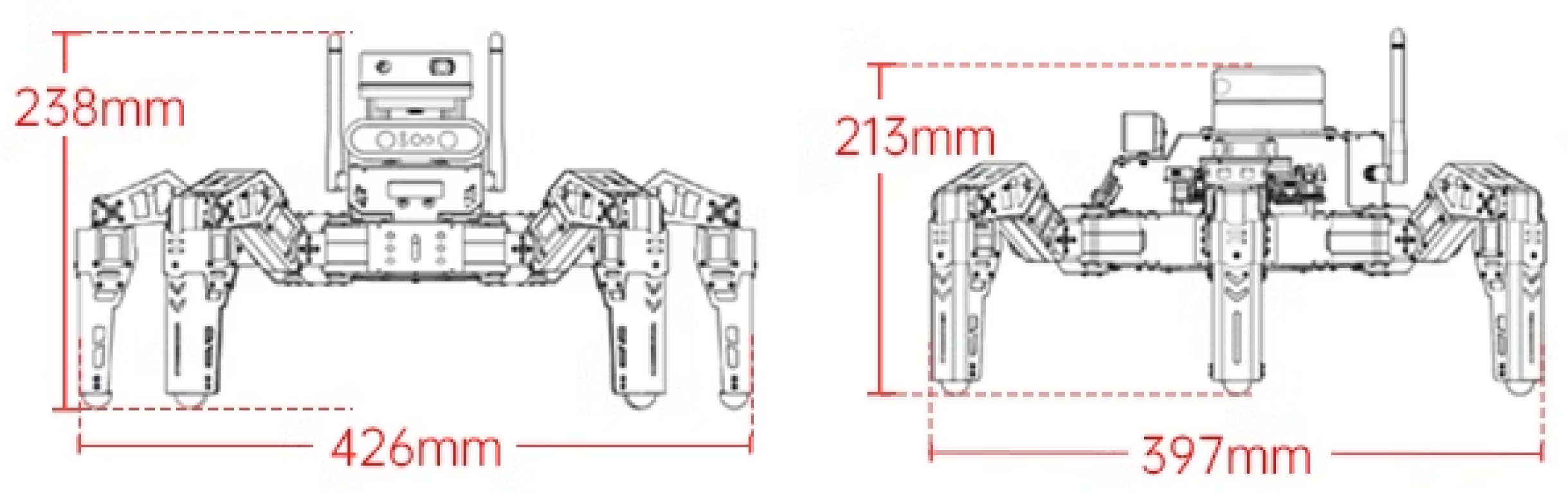
The structure of the experimental hexapod robot in this paper is shown in
Figure 1, in which the overall length of the hexapod robot is 397 mm, the width is 426 mm, and the height is 238 mm. The forward direction of the robot is the
X-axis positive direction, the
X-axis positive direction rotated counterclockwise by 90° is
Y-axis positive direction, the vertical upward is the
Z-axis positive direction, and the unit of measurement is mm. The coordinates of each joint are shown in
Table 1.
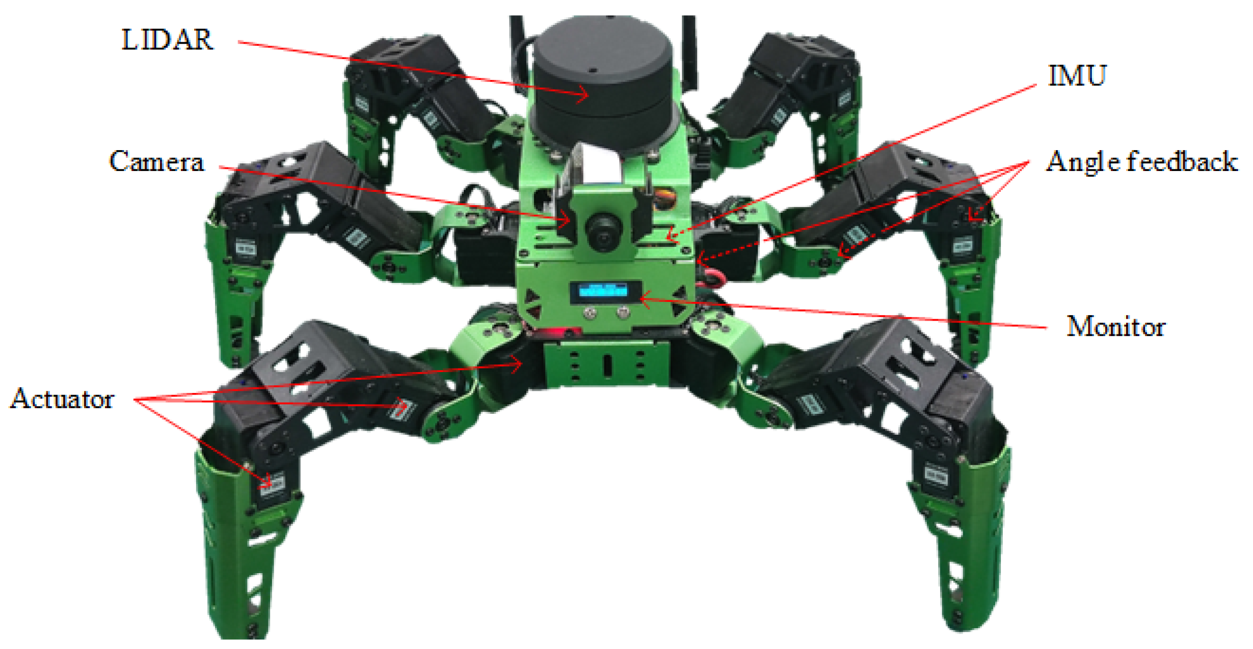
Each leg joint of the hexapod robot consists of a high-voltage servo, an angle feedback device, and a temperature and voltage sensor. The angle feedback device can record the rotation angle of each joint, and the temperature and voltage sensor can understand the internal data of the servo in real time, to protect the servo. As shown in
Figure 2, the hexapod robot has an inertial measurement unit (IMU) and an 18-angle feedback as proprioceptive sensors, which form the sensor network of the hexapod robot.
2.2. Control Framework
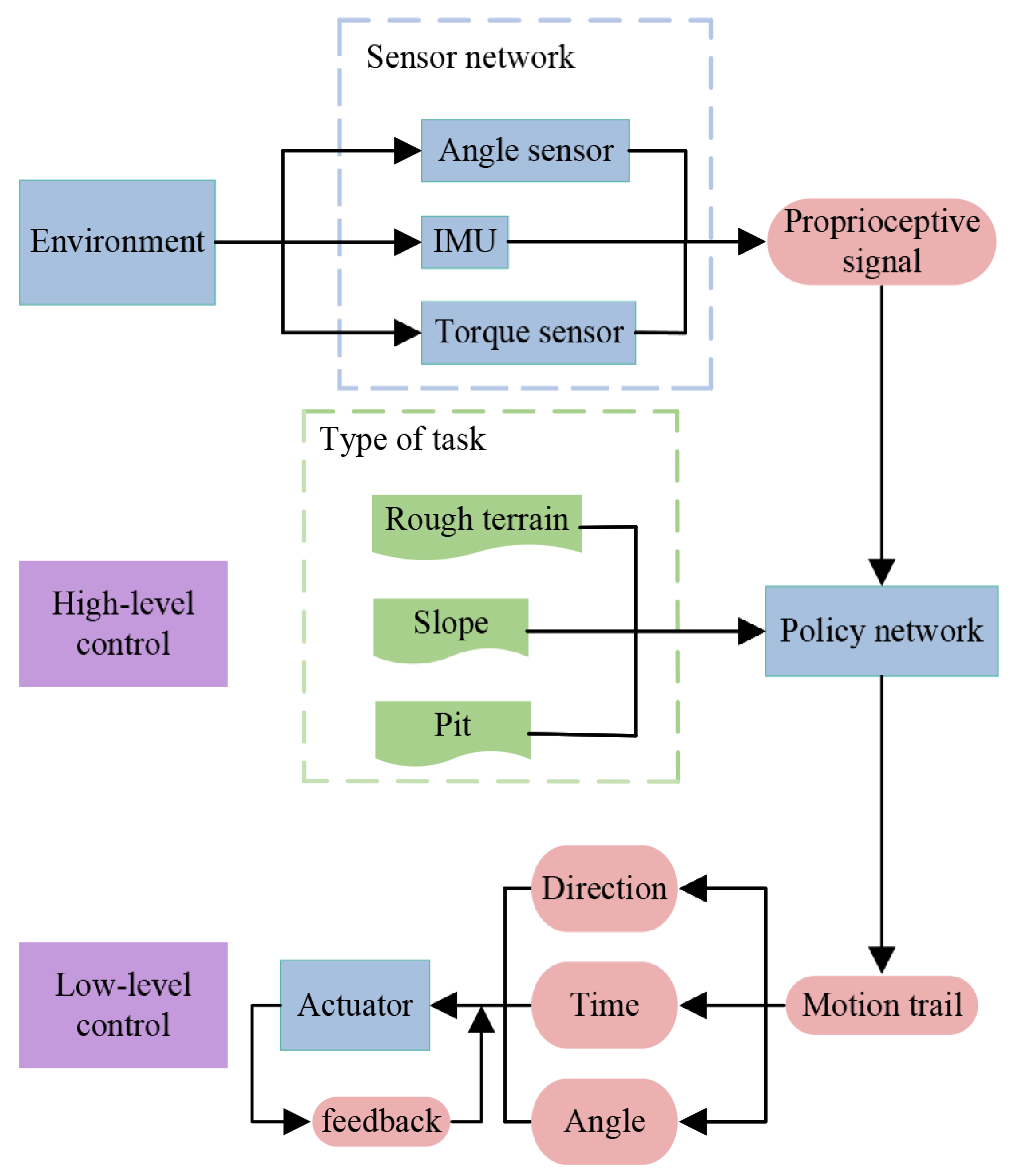
As shown in
Figure 3, the control framework can be mainly categorized into two stages: low-level control, and high-level control. First, the proprioceptive signals are obtained from the environment through the sensor network, which can determine its own attitude and the ruggedness of the surrounding environment. In the high-level control, the policy network receives the human-selected task types and proprioceptive signals, and then it generates robot trajectories and gaits corresponding to the tasks. In the low-level control, the motion trajectory of each joint of the hexapod robot is decomposed into angles and motion directions at certain time intervals, and finally the joints are precisely rotated by the positional PID control through feedback from the angle feedback device.
2.3. Adaptive Gaits
The motion of a hexapod robot is a high-dimensional combinatorial problem, and the best solution is to choose a suitable gait for a given terrain. A gait is a periodic motion that restricts the robot’s movements to the appropriate terrain. A suitable gait ensures that the robot can traverse the terrain without damaging itself or the terrain, and is superior in terms of energy efficiency and smoothness. An appropriate gait is capable of crossing a given terrain with minimal movement, i.e., minimal wear and tear on the joints.
On structured terrain, a single gait can be used to pass through the terrain. The unstructured ground is complex and has many obstacles, and using adaptive gait allows the hexapod robot to autonomously fine-tune its gait according to its surroundings, to adapt to the unstructured ground. In this work, adaptivity is a locomotion strategy for a hexapod robot that relies only on proprioceptive signals to recognize information about its surroundings and thus change its entire gait.
2.4. Walking and Obstacle Avoidance
The blind hexapod robot exploits internal sensors to obtain information about its surroundings, which include an inertial measurement unit IMU on the torso, and angle feedback and torque feedback at each joint. The proprioceptive signals from the hexapod robot can be obtained after integrating the signal processing of the internal sensors. Proprioception is the perception of one’s own space and position in three-dimensional space, and this also allows the body to perceive changes in limb movements [
41]. For example, blind people are able to carry out normal behavior such as walking and eating through proprioception and touch even though they have lost their vision. Simple or complex sports such as walking, running, and playing basketball require proprioception [
42]. The proprioceptive signals obtained from the sensor network are the trunk position, trunk linear velocity, trunk angular velocity, joint angle, and joint angular velocity.
The hexapod robot–environment interaction is discretized in the time dimension as a sequence of time steps. The state of the hexapod robot with the environment at each time step is represented by the vector
s, which contains all proprioceptive signals acquired from the sensor network. The reward obtained by the hexapod robot interacting with the environment at each time step is denoted by
r, which reflects how favorable the current environment is to the robot. The action performed by the hexapod robot at each time step is denoted by the vector
a, which contains the motion trajectories of all the moving joints. As shown in
Table 2, the interaction process between the hexapod robot and the environment is described using MDPs. When the hexapod robot walks on rugged ground, the state of each time step changes with the roughness of the terrain. As shown in
Figure 4, the rougher the terrain, the larger its stance angle, and the drop of each leg is larger, thus adjusting the gait to adapt to the environment. In particular, when the hexapod robot is walking on high slopes or pitted terrain, its stance angle rises or falls sharply in succession. When it encounters an impassable high slope or pit, it can make an evasive maneuver at the next time step, according to the change of attitude angle.
3. A Soft Actor-Critic Algorithm
The interaction process between the hexapod robot and the environment uses MDPs, which satisfy the conditions for the use of RL. This paper uses SAC to train the motion strategy of the hexapod robot. SAC is a non-strategy DRL based on maximum entropy, where the introduction of maximum entropy gives a strong exploratory ability [
43]. In addition, it has excellent robustness and high sampling efficiency, providing a stable learning framework for control tasks in continuous action space [
44].
SAC has an additional entropy term
compared to the objective function of conventional DRL:
is
where
is the distribution of
x. The maximum entropy term makes the action output more random, thus improving the exploration and learning ability of the algorithm. Then, the optimal policy
in SAC is
where
is the robot’s motion strategy,
a denotes the action,
s denotes the state, and
r denotes the reward. Here,
denotes the temperature coefficient, a hyperparameter that determines the importance of entropy with respect to the reward, thus controlling the degree of randomness of the strategy.
Set the state
and the action
at time
t, and the value function
is
where
is the discount coefficient.
As for actor-critic, SAC has value networks and policy networks. To avoid using an overestimated
Q network to compute the objective when maximizing, SAC introduces two online networks and two objective networks. The parameters of the two online networks are set as
and
, and the parameters of the two target networks are set as
and
. Then, the minimum value of the output of the two target networks are obtained as the target value in the calculation. The parameters of the value network can be updated by minimizing the loss function as
The policy network parameters are denoted by
, with the state
as input. A Gaussian distribution with mean
and standard deviation
is used as the output. Then, the action
can be obtained using a reparameterization with
as
In the above formula, the
function outputs the mean and standard deviation,
is the standard normally distributed noise signal, and
and
are the mean and standard deviation of the Gaussian distribution, respectively.
SAC represents the policy with an energy-based model, which is an appropriate solution for difficult control tasks. To establish a link between the energy model and the soft value function, it is necessary to set a suitable energy function, and the energy function
is set as
Then, the policy
can be expressed as
The policy network parameters are updated using a method that minimizes the Kullback–Leibler scatter. When the Kullback–Leibler scatter is smaller, the difference between the corresponding output behavioral rewards is smaller, and the policy converges better. The update function of the strategy network is
where
is used to normalize the distribution.
Finally, the parameters of the policy network are updated using the gradient descent method, denoted as
The larger the temperature coefficient
, the stronger its exploration ability. The adjustment of the hyperparameter
has a great impact on the training effect of the SAC, and
needs to be adjusted for different tasks and different training cycles. A temperature auto-adjustment mechanism [
45], which obtains the optimal temperature coefficients for each step by minimizing the objective function, is denoted as
where
is a predefined threshold for the minimum policy entropy. Algorithm 1 gives the pseudo-code for the SAC.
| Algorithm 1 The training method of SAC |
Input: initial a empty experience memory M and iteration number N. Output: policy network - 1:
initial parameters , , - 2:
initial target network parameters , - 3:
for N do - 4:
for each environment step do - 5:
Observe state and select action - 6:
Execute , observe next state , reward - 7:
Store in the experience memory - 8:
end for - 9:
for each gradient step do - 10:
Randomly sample a batch of samples from M - 11:
Update Q-functions parameters: - 12:
for - 13:
Update policy parameters: - 14:
- 15:
Update temperature coefficient: - 16:
- 17:
Update policy network parameters: - 18:
for - 19:
end for - 20:
end for - 21:
return policy network
|
4. Training Procedure
This chapter first introduces Mujoco, a training platform for blind hexapod robots, then, describes its process for training policy networks.
4.1. Training Platform
RL tends to require more samples than supervised and unsupervised learning. Because the training process of RL requires a large number of interactions and trials, it must constantly interact with the environment. This leads to some limitations in the application of RL in real time, especially when the real environment is costly or risky [
46].
Using virtual environments for training is the preferred solution. Robots may encounter unexpected situations in the real world, which can lead to the destruction of equipment, injury, or other unforeseen consequences. By training in a virtual environment, potential risks can be avoided, and this ensures that the trained strategies are more reliable and safe when used in a real environment. The physics engine also provides complete control over the environment and tasks. It is easy to modify the parameters of the virtual environment, introduce different scenarios and contexts, and perform fast playback and replay. This makes RL debugging and optimization easier and more efficient. More importantly, training in a virtual environment provides easy access to rich data, including states, actions, and reward signals. These data serve as datasets for algorithms to perform model learning and strategy optimization. In addition, the physics engine records and saves detailed information of each training step for subsequent analysis and evaluation.
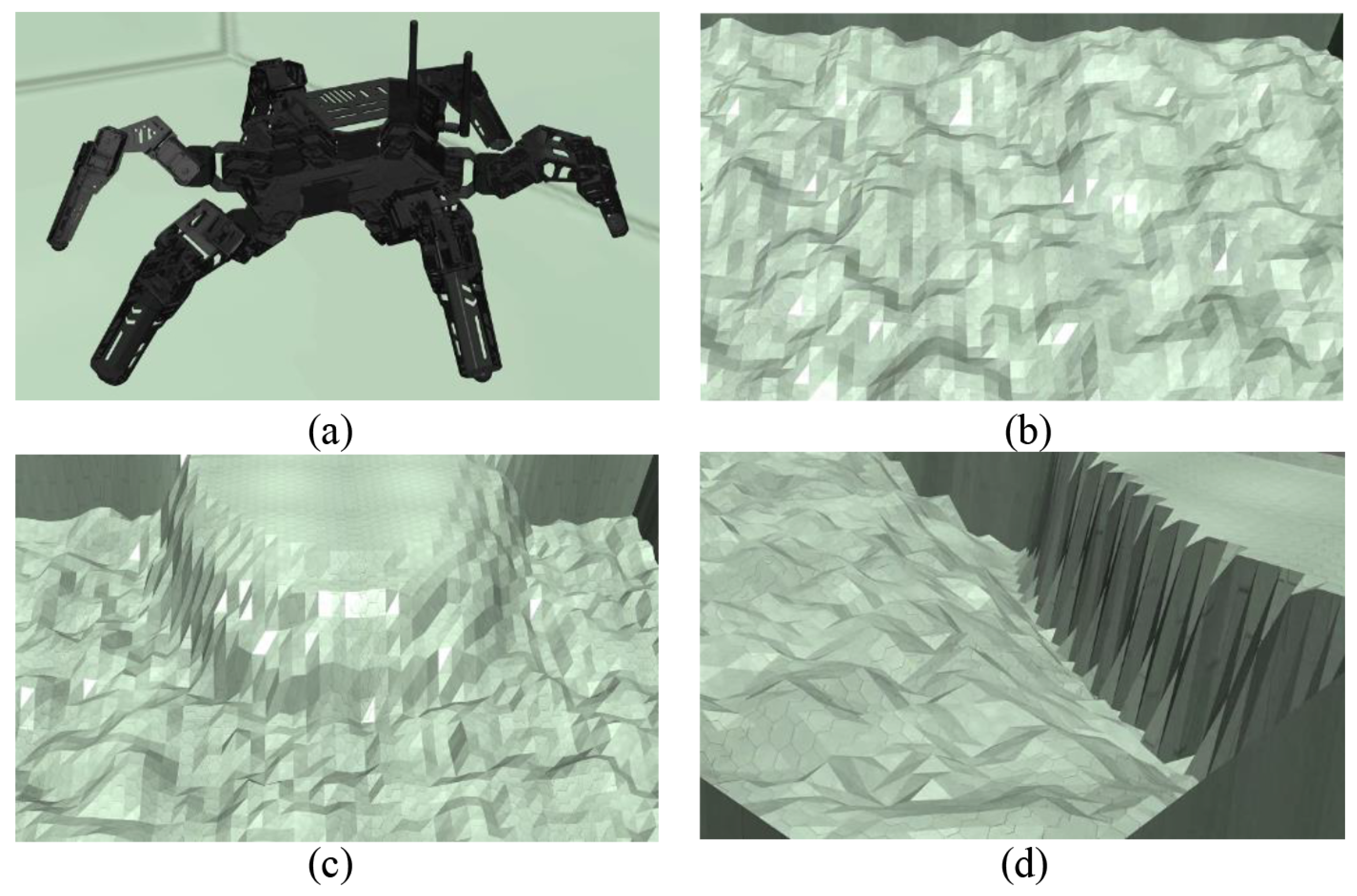
This paper established a training platform for hexapod robots using Mujoco [
47], a commonly used physics simulation engine that is widely used in robot control, reinforcement learning, and motion planning. It is able to simulate the dynamic behavior of rigid body systems with multiple joints and contact forces. It is based on Newtonian mechanics, to calculate the collision, contact force, and dynamic behavior between objects. The geometry, inertial properties, and joint types of a hexapod robot are described through XML files. The terrain is represented by a grayscale map with topographic information. At the same time, the geometry, surface friction, and collision characteristics of the terrain are also represented by XML files and generated in MuJoCo.
Figure 5 shows a simulation model of the hexapod robot and terrain.
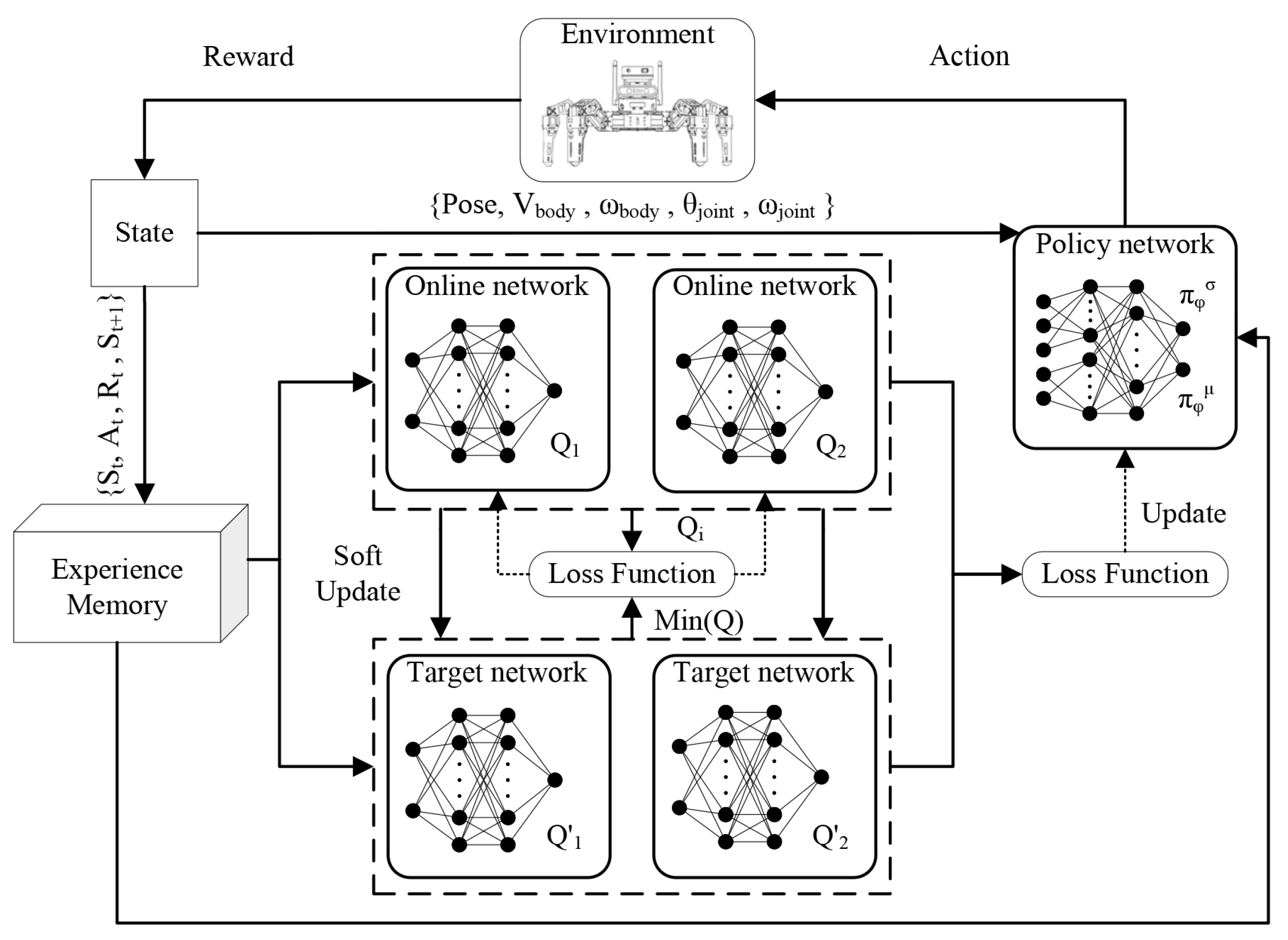
4.2. Training Framework
Figure 6 shows the control framework of the hexapod robot based on SAC. SAC is implemented using pytorch and trained using Mujoco-py, to control the simulation environment. The state space contains all proprioceptive signals, including the torso position Pose, torso linear velocity
, torso angular velocity
, joint angle
, and joint angular velocity
. Then, the state space vector
S is
The action space contains the motion trajectories of 18 joints used to control the robot and is represented by the vector
A:
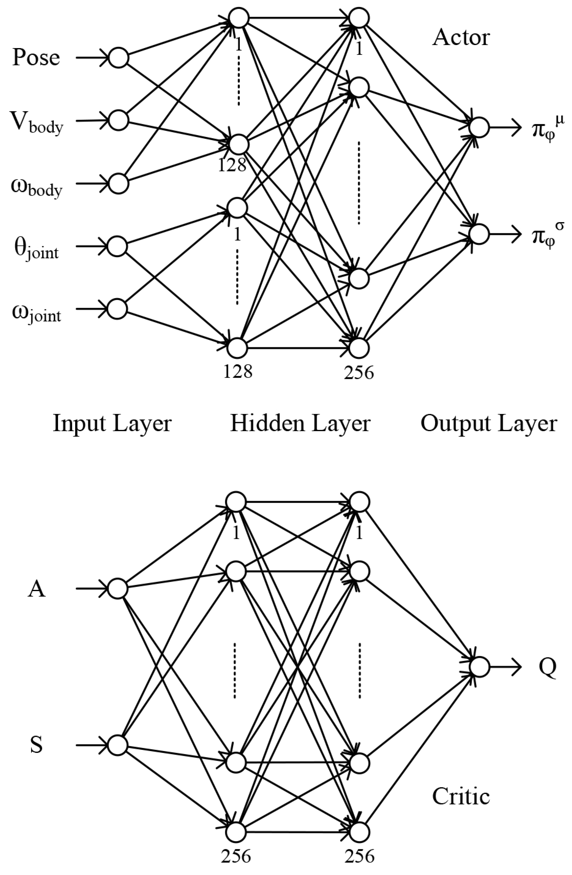
The neural network structure used by SAC is shown in
Figure 7. In this paper, the structure of the actor is modified. Two micro-neural networks are first used to extract features for highly relevant inputs, and then the features are put into a fully connected neural network. The actor uses a strategy network containing four layers, with the first input layer and the second hidden layer consisting of two micro-neural networks, as the input and output layers of the micro-neural network, respectively. The first micro-neural network input layer is
,
and
, and the output layer has 128 torso-related features. The second micro-neural network input layer is
and
, and the output layer has 128 leg-related features. The third layer of the strategy network is a hidden layer containing 256 units that combines the features extracted by the two micro-neural networks. The fourth layer is the output layer, which outputs the mean
and the standard deviation
of action obeying a Gaussian distribution. The critic, on the other hand, uses two online networks and two target networks with the same structure, the first layer being an input layer containing 64 units with inputs
A and
S, the second and third layers having the same structure as the actor’s hidden layer, and the fourth layer being an output layer that outputs the
Q value, to evaluate the current action.
The reward function needs to be set according to the specific task and environment. When the hexapod robot is trained to walk on rugged ground, the total reward
consists of reward
and penalty
, which is given by the expression
The speed reward
encourages the robot to move forward, and the closer it moves to the set speed
the greater reward it will receive. If the reward function is given as the travel distance to the goal, training results in an unstable or jumpy gait, and this makes the training time much longer. Let the current speed of the robot in a single step be
v, and
be set to
To ensure the correctness of the hexapod robot’s heading, the penalty
is set to correct the heading. Quaternions are in the complex form of Euler angles, which decompose the rotation of an object into a rotating vector and a rotating angle. If the rotating angle of the hexapod robot is denoted by
, then
is set as
An additional penalty
is required for training a hexapod robot to avoid obstacles; utilizing the fact that the pitch and roll angle of robot changes drastically when it is going up a steep slope or going down a steep slope. This change can be sensed by the propriety sensors, which are utilized to allow the robot to avoid specific obstacles. Then, the penalty
and total reward
are set as
In this framework, the input to the policy network is the state space vector and the output is the mean and standard deviation obeying a Gaussian distribution. The action space vector is then generated using a reparameterization method. The reward and the generated action after evaluating the environment are then fed back to the hexapod robot to enter the next state . The current state, action, reward, and next state are composed into an experience vector , which is stored in an experience memory. For training, a small batch of experience samples are randomly selected from the experience memory, to iterate on the network parameters of the online network, and a soft update method is used to iterate on the parameters of the target network and policy network.
5. Testing Results
In this paper, slightly modified SAC, PPO, and TD3 were used to train the hexapod robots during the training process, and the training results are shown in
Figure 8. SAC and TD3 had a higher degree of exploration, so the rewards obtained in the pretraining period were much lower than those of PPO. The adaptive parameters introduced by SAC struck a balance between maximizing the expected cumulative reward and minimizing the entropy of the strategy. Adaptive temperature parameters can better adapt to different tasks and environments, and improve the performance of the algorithm. As a result, the rewards obtained after the convergence of SAC in the later stage were higher than for PPO.
Figure 8 above shows that TD3 overfitted when trained for this task, and its reward maximum point was lower than with SAC. In summary, the modified SAC training was optimal for this task.
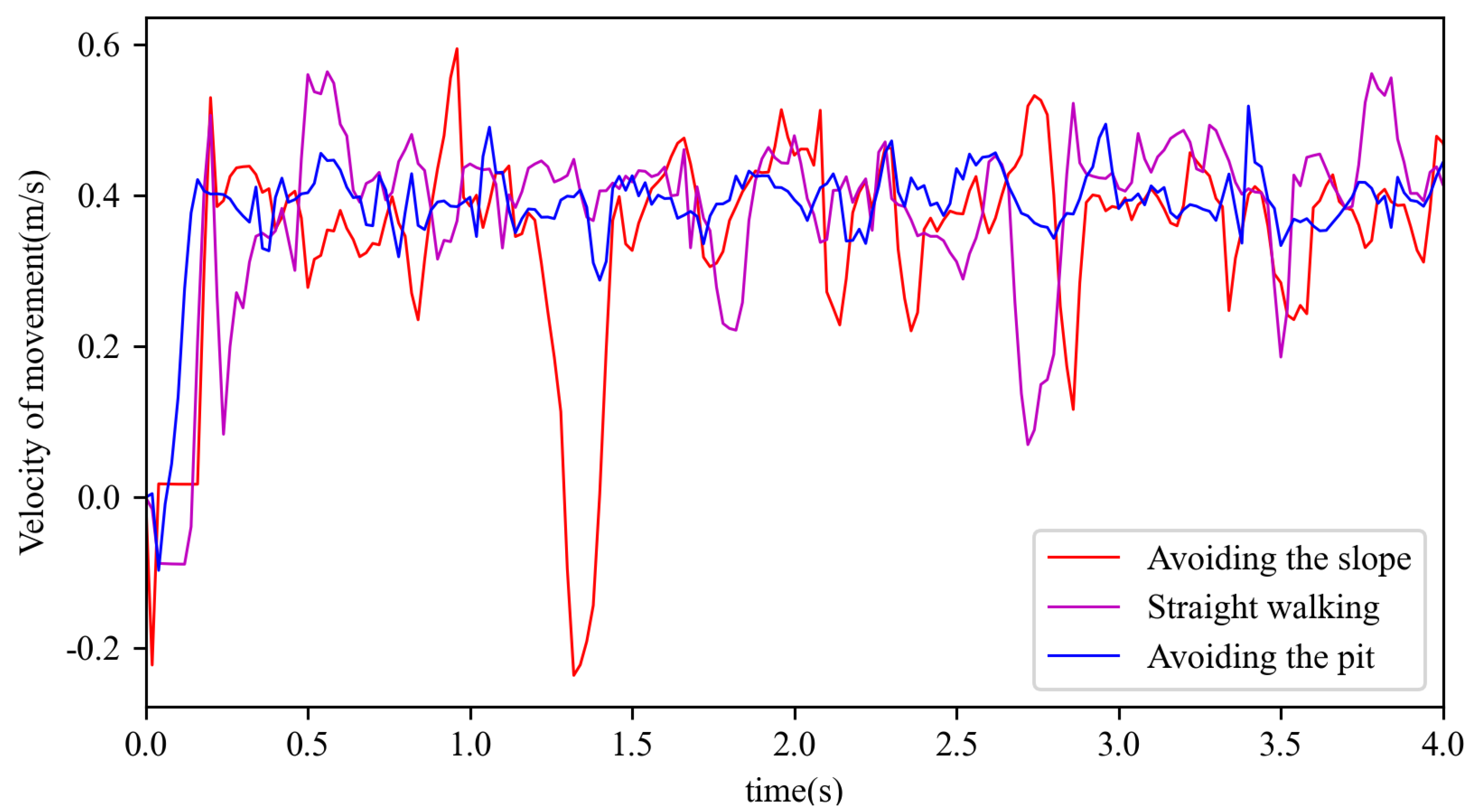
One objective of training a hexapod robot is a fixed walking speed, because the robot needs the right walking speed, no matter what terrain it is on. In this paper, the speed was set to 0.4 m/s for all three terrains of the training, or different speeds could be set separately. The walking speed of the trained hexapod robot is shown in
Figure 9. In all three terrains, the robot started moving from rest, so the initial speed was 0 m/s. Then it accelerated to 0.4 m/s after an acceleration process of about 0.4 s, and stayed at about 0.4 m/s. Since all three terrains were rough terrains, the speed kept oscillating around the target speed. There was a strong deceleration process and acceleration process at around 1.3 s during the robot’s movement on the slope. The slowdown was due to the impassable slope, which hindered movement. After being blocked, the hexapod robot gradually changed its direction of movement, bypassed the slope, and accelerated to about 0.4 m/s, to continue walking.
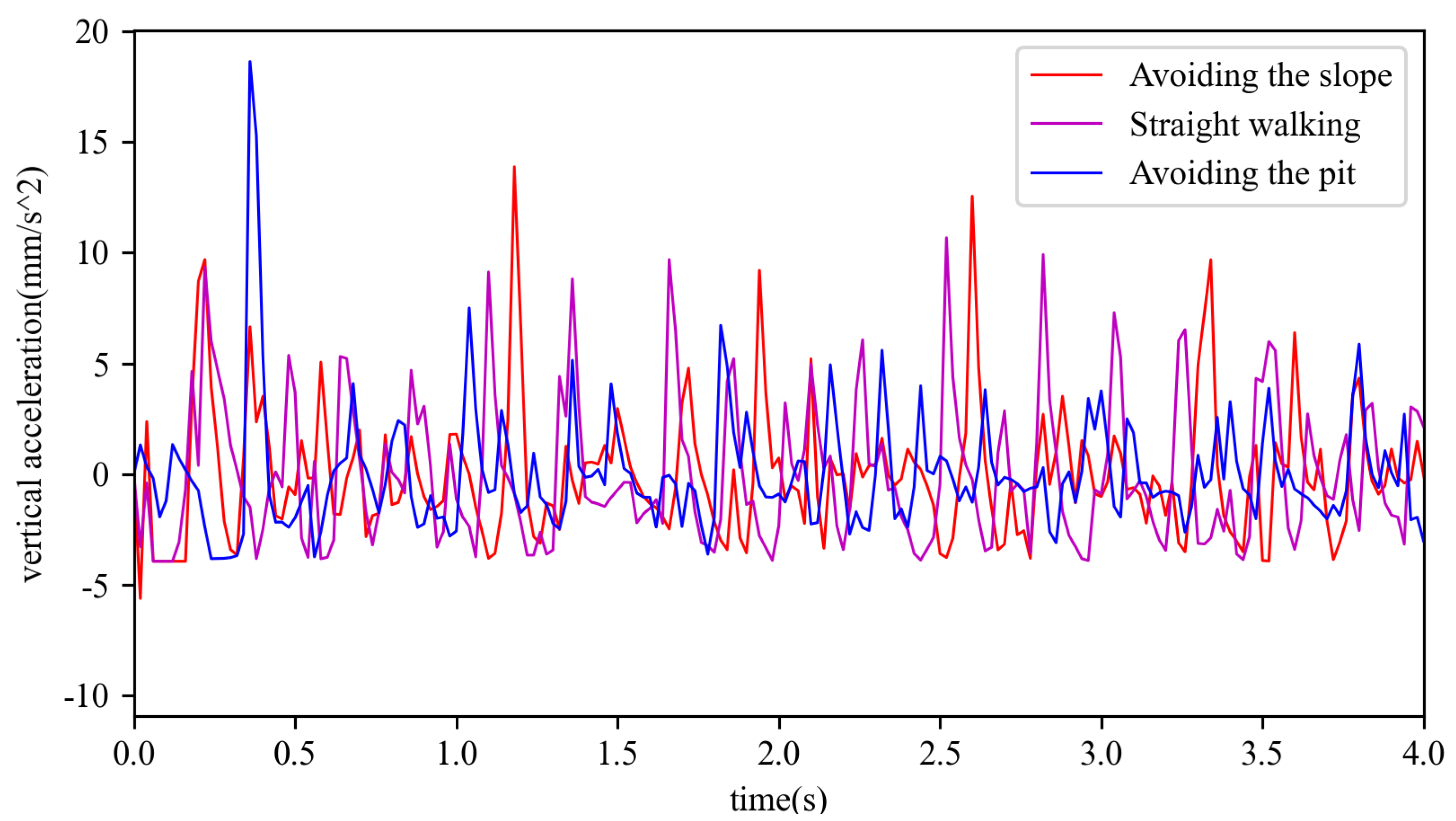
In this paper, the stability of robot motion was judged on the basis of the vertical acceleration, oscillations around roll, and oscillations around pitch during the motion process.The vertical acceleration during the motion on the three terrains is shown in
Figure 10, and the vertical acceleration of the robot kept oscillating from around 0 at the beginning of the stationary motion to the uniform motion, and its amplitude mostly kept in the range of 5 mm/s
to 10 mm/s
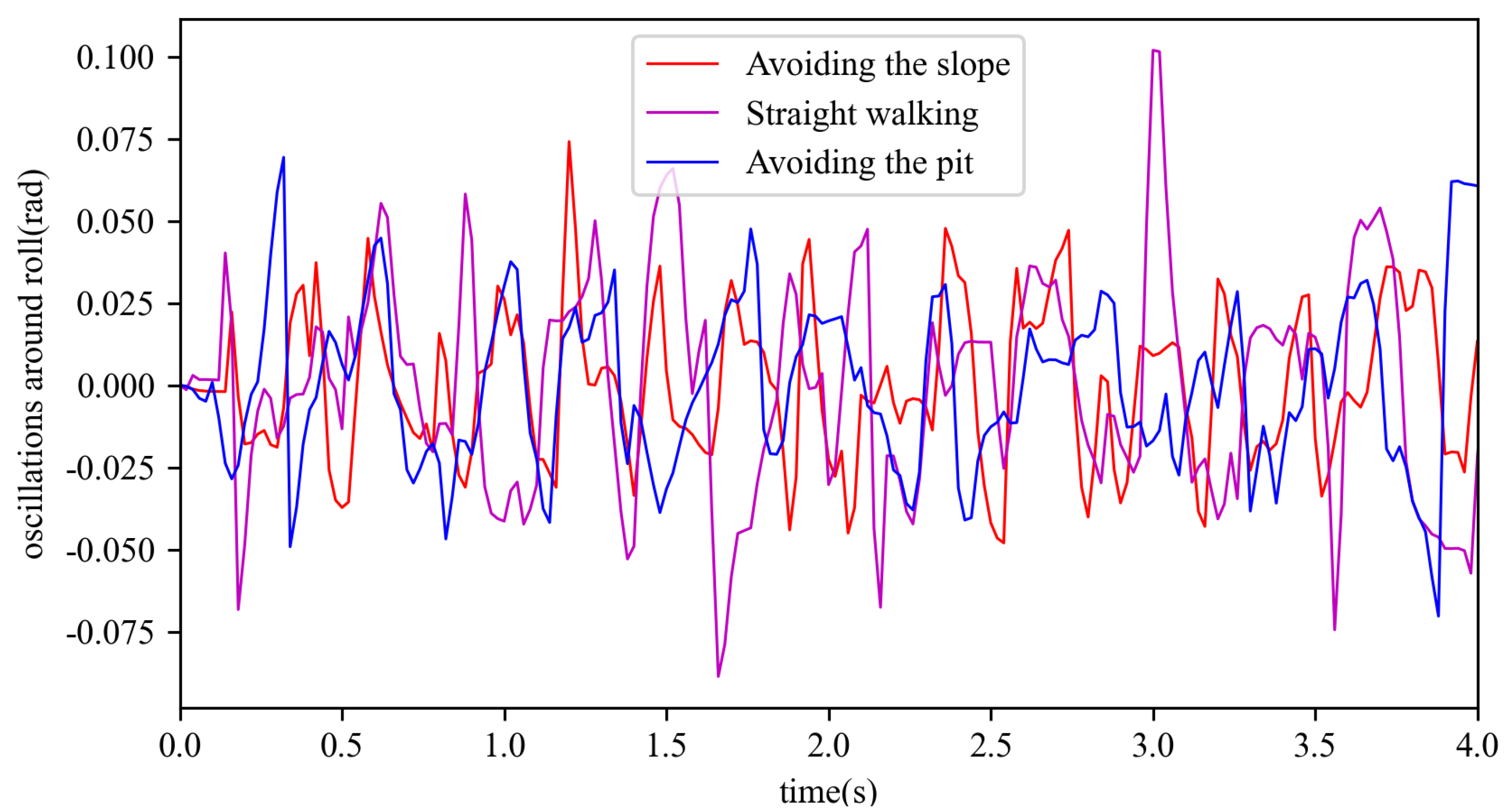
. The robot showed a large change at about 0.4 s during the pit movement, since the robot moved to the edge of the pit and changed its direction of movement. The standard deviation for avoiding the slope was 3.05 mm, the standard deviation for straight walking was 3.24 mm, and the standard deviation for avoiding the pit was 2.67 mm. The oscillations around roll during the motion on three terrains are shown in
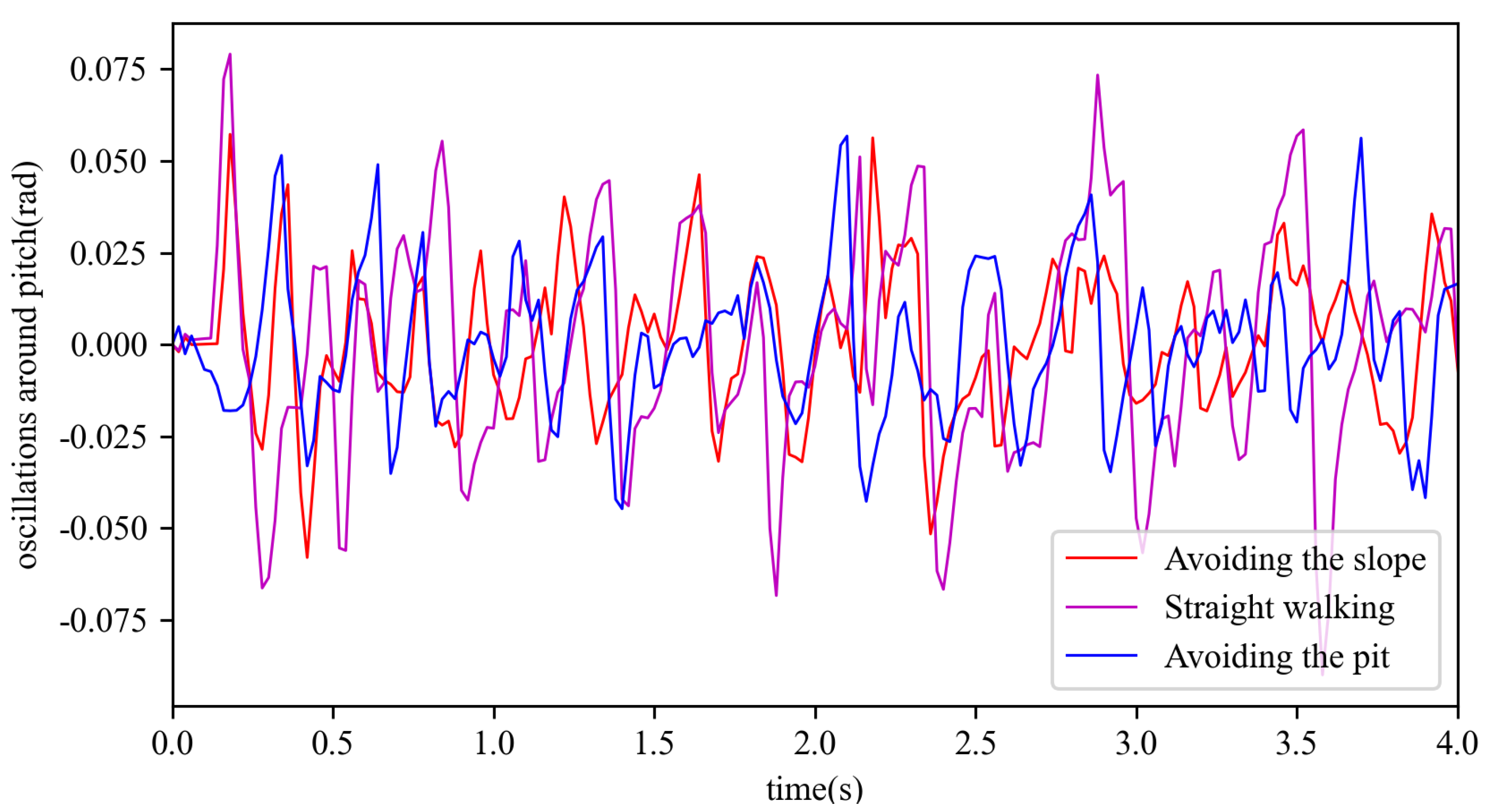
Figure 11. The standard deviation for avoiding the slope was 0.023 rad, the standard deviation for straight walking was 0.033 rad, and the standard deviation for avoiding the pit was 0.025 rad. The oscillations around pitch during the motion on three terrains is shown in
Figure 12. The standard deviation for avoiding the slope was 0.020 rad, the standard deviation for straight walking was 0.031 rad, and the standard deviation for avoiding the pit was 0.020 rad. From these figures, it can be seen that the standard deviations of vertical acceleration, oscillations in pitch, and oscillations in roll were small and the stability was acceptable.
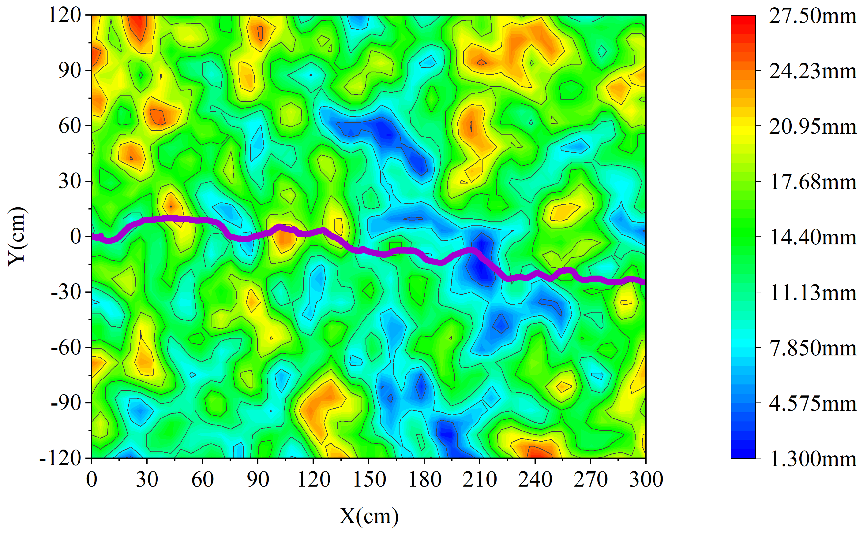
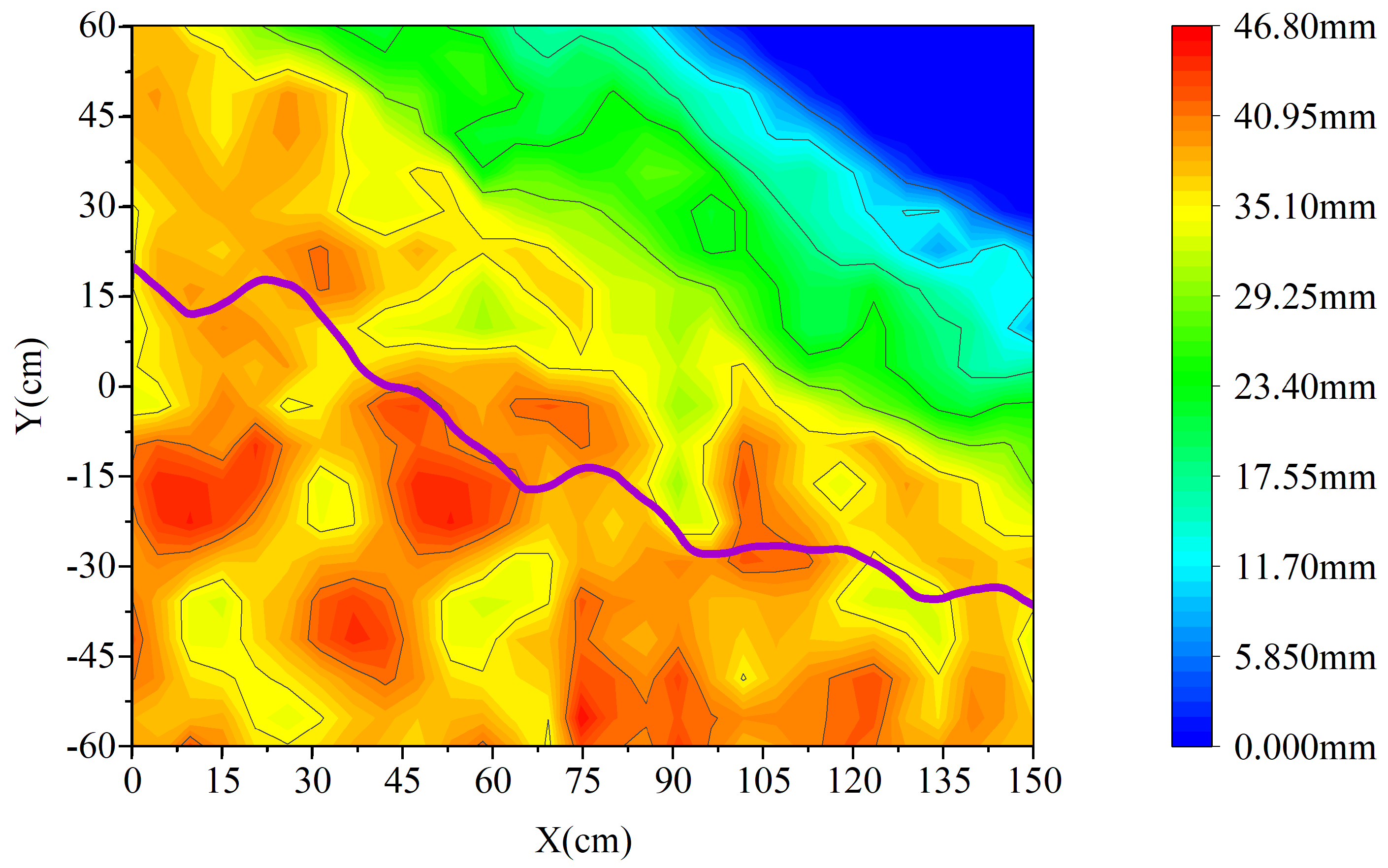
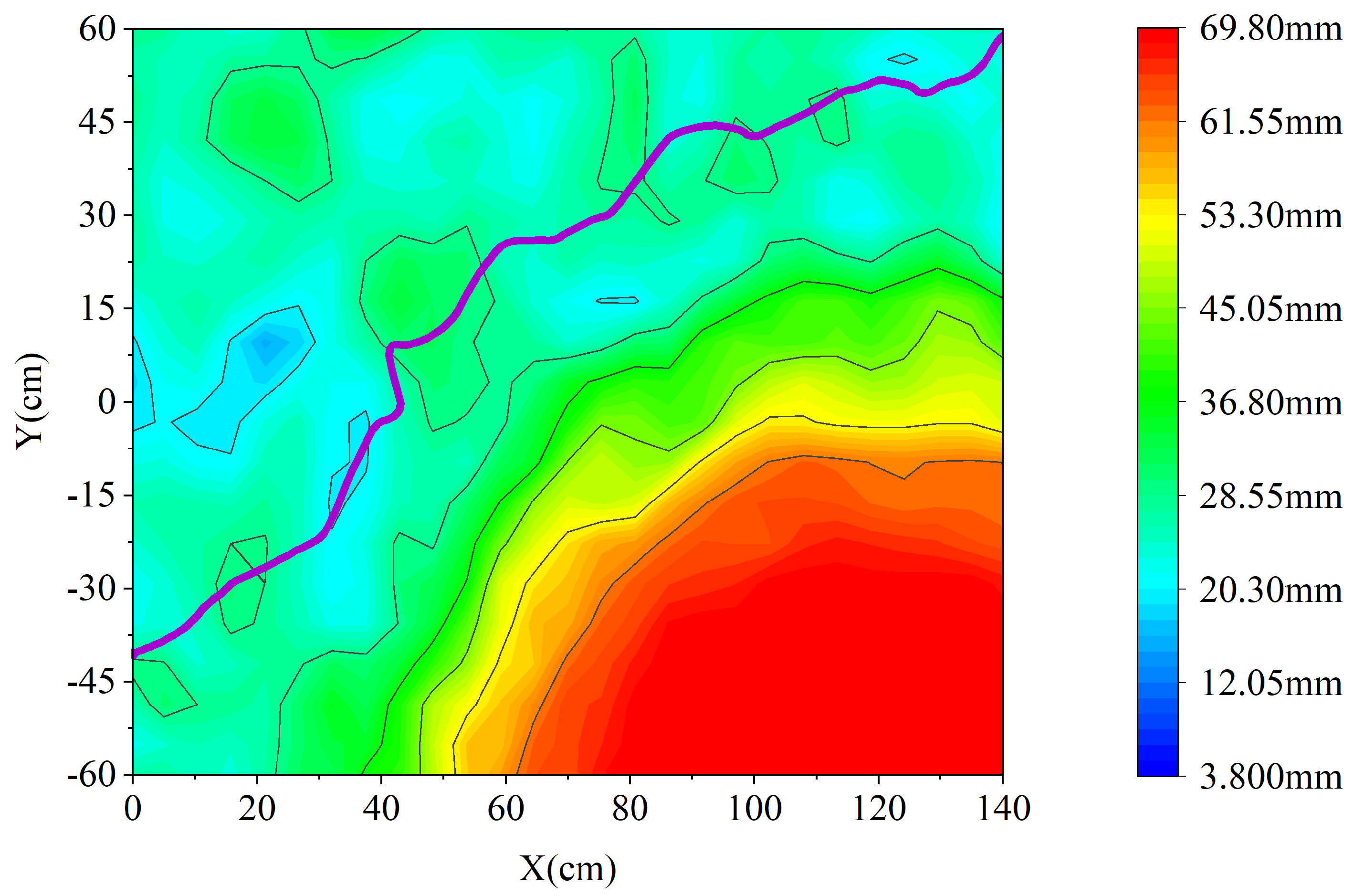
In this paper, contour maps were used to describe the paths of the hexapod robot moving over the three terrains. The purple curve represents the change in the center of gravity, and the color shading represents the altitude gradient.
Figure 13 shows the motion path of the robot on perlin, for which the motion path of the robot was straight within a deviation of ± 25 cm.
Figure 14 shows the motion path of the robot when avoiding pits; in the figure, the robot detects the pit at around x = 22 cm and then keeps moving towards the edge of the pit without stepping into it.
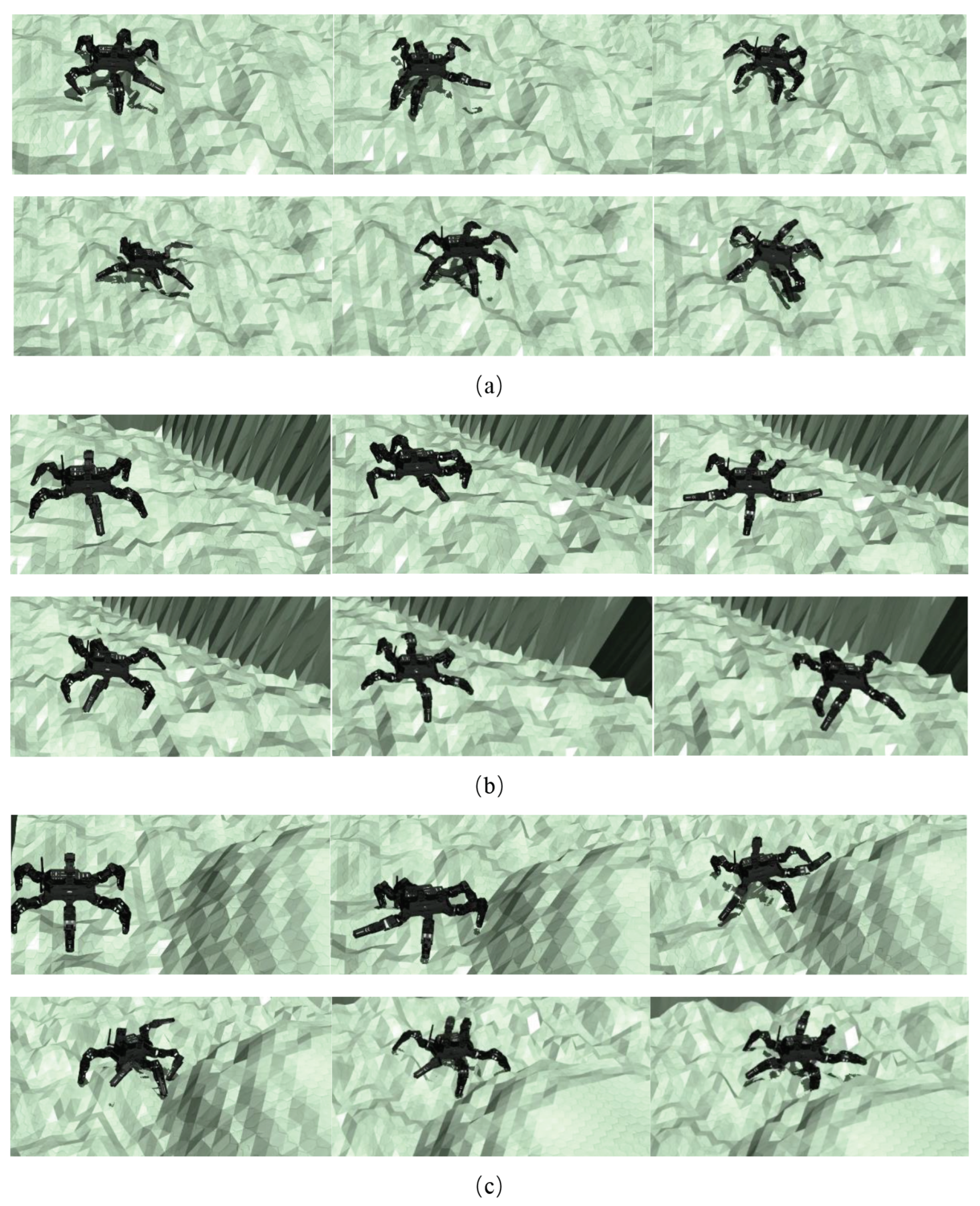
Figure 15 shows the motion path of the robot when avoiding the slope, in which the robot detects the slope at about x = 30 cm, and then changes the direction of motion towards the top. In summary, the hexapod robot in this paper has the ability to walk and avoid obstacles in rugged terrain, and
Figure 16 shows the performance of the hexapod robot in the simulator.
6. Conclusions and Future Work
This paper presented a control method for a hexapod robot, which not only allows the hexapod robot to be protected from weather and light while performing tasks in the field, but also to avoid specific obstacles. A modified strategy network actor is used as the robot’s motion strategy, which is obtained through SAC training. Due to the different tasks, the corresponding policy networks need to be trained separately, and corresponding physical environments are established, which should be consistent with the actual environment as much as possible. The trained strategy network can only rely on proprioceptive sensory signals to command the hexapod robot to perform adaptive movements, and realize stable walking at a specific speed and pass through the rugged ground, as well as a certain obstacle avoidance ability. This provides a solution for the movement control of hexapod robots in wild mountains. A scheme is provided for the motion control of a hexapod robot in wild mountainous areas.
The method given in this paper requires manual selection of a specific policy network when facing different terrains. In future work, we will train a network so that the robot learns to classify terrain and choose the best motion strategy during movement. The network enables the machine to adapt to a variety of terrain combinations [
48,
49]. ILC is a control method that optimizes the current system based on historical experience. Optimization of the robot’s end-of-foot trajectory, in conjunction with ILC, could be used to improve the robot’s locomotion performance [
50,
51]. In addition, shared control combines human intelligence and robot intelligence, and the framework could fully utilize the advantages of human–robot collaboration to better train the strategy network [
52].


