Abstract
Trailing-edge noise (TE noise) is an aeroacoustic sound radiated from an isolated airfoil in the specific ranges of low-speed flow. We used a pulsed laser as an actuator to reduce the TE noise without modifying the airfoil’s surface. The wind tunnel test was conducted to verify the capability of an Nd:YAG laser as the actuator. The laser beam was focused into the air just outside the velocity boundary layer on the lower side of an NACA0012 airfoil. The experimental result shows that the TE noise is suppressed for a certain period after beam irradiations. We then analyzed the physical mechanism of the noise reduction with the laser actuation by the implicit large eddy simulation (ILES), a high-fidelity numerical method for computational fluid dynamics (CFD). The numerical investigations indicate that the pulsed energy deposition changes the unstable velocity amplification mode of the boundary layer, the source of an acoustic feedback loop radiating the TE noise, to another mode that does not generate the TE noise. The sound wave attenuation is observed once the induced velocity fluctuations and consequently generated vortices sweep out the flow structure of the unstable mode. We also examined the effect of the laser irradiation zone’s shape by numerical simulations. The results show that the larger irradiation zone, which introduces the disturbances over a wider range in the span direction, is more effective in reducing the TE noise than the shorter focusing length with the same energies.
1. Introduction
Aviation demands have risen more than ever before, and developing advanced noise reduction technologies has become important to ease the noise of aircrafts impact around airports [1]. In certain flow conditions, an aircraft wing radiates a sound wave as a consequence of the interaction between an unsteady flow over the walls and the rear edge, known as the trailing-edge noise (TE noise), a part of the noise of an aircraft. Significantly, in specific angles of attack (AoA) and moderate Reynolds numbers conditions at the low-speed regime, the instabilities of the laminar boundary layer form intense vortex shedding that generates characteristic tonal noise [2,3]. This type of TE noise is defined as the laminar boundary layer vortex shedding (LBL-VS) type trailing-edge noise [4,5]. In this study, we consider the LBL-VS type of TE noise.
Many pieces of previous research have investigated the physical mechanism of the LBL-VS type of TE noise since the early 1970s [2,3,4,5,6,7,8,9,10,11,12,13]. Figure 1 schematically depicts the source of the TE noise. The self-sustained discrete tone is maintained by an acoustic feedback loop consisting of the velocity instabilities of the laminar boundary layer, known as the Tollmien-Schlichting (TS) wave, and the sound wave from the trailing edge [6,7,8]. The sound wave (and disturbances in the surrounding flow) initially excites the velocity fluctuations in the boundary layer on the airfoil fore part [13], and the induced fluctuations grow as the TS wave flows ahead to the trailing edge. The dominant frequency of the TE noise agrees with the TS wave frequency estimated from the linear instability theory [3,7,12]. Previous studies [3,12] have indicated that the lower side laminar separation bubble also plays an essential role in the velocity amplification and in selecting the dominant frequency. The vortices generated by the TS wave interact with the trailing edge. Consequently, the vortex sound is radiated as the TE noise. The sound wave propagates to the upstream direction and excites the boundary layer again. This acoustic feedback loop maintains the generation of noise and also contributes to secondary tones around the main tone frequency [3,8,14].
Figure 1.
Schematic diagram of the generation of trailing-edge noise.
The TE noise mechanism indicates that adequately controlling the TS wave can reduce the noise. Some flow control techniques have been suggested to reduce the TE noise [15,16,17,18,19,20]. One effective way of noise control is to deform the wall shape using the piezoelectrically driven oscillating surface (PDOS) actuator [15,16]. Wylie et al. [16] used a PDOS actuator placed on the upper side surface to cancel the TS wave by introducing an anti-phase disturbance. A closed-loop control with an iterative learning algorithm drove the actuator and reduced the TS wave’s amplitude. Another effective device is a dielectric barrier discharge plasma actuator (DBDPA) [17,18]. Simon et al. [19] constructed a feedforward control system for a manned glider airfoil consisting of a DBDPA and two hot-wire flow probes placed upstream/downstream of the actuator. The control system suppressed the TS wave 12–15 dB compared to its uncontrolled state at the flight speed of 40 m/s. It is noteworthy that the system attenuated disturbances over a wide frequency band centered on the dominant frequency. A periodical flow injection/suction was also suggested as an alternative control method with extremum-seeking control (ESC) scheme [20]. We note that we can easily break the acoustic feedback loop by tripping the boundary layer to turbulence, but it also leads to a drag increase [21]. What we wish to achieve is a reduction in the TE noise while retaining the lift-drag characteristics.
Although the methods mentioned above sound suitable for controlling the TE noise, they are hard to install since they invade the airframe’s structure and might weaken the structural robustness. Recently, the pulsed laser has been employed as a contactless actuator for the flow control. Several studies have shown that laser-based energy deposition approaches can be a practical flow control application [22,23,24]. The impulsive energy deposition afforded by the rapid heating of the laser pulse causes a unique thermal/density distribution [22]. Kim et al. [23] experimentally demonstrated the wave drag reduction by repetitive laser energy depositions onto a shock wave/boundary layer interaction region in a supersonic flow. Bright et al. [24] conducted an experimental study to control the laminar separation on an airfoil using a remotely located laser deposition. They showed that a laser beam focused through a convex lens induced an air breakdown near the upstream of the leading edge. Enhancing the momentum transfer from the surrounding flow to the boundary layer due to the heated air caused the flow reattachment. Keeping in mind that the laminar separation bubble contributes to the emission of TE noise, this work gives us the impression that the pulsed laser could control TE noise as the previous research did.
In this study, we employed a pulsed laser as an actuator to reduce TE noise. Section 2 presents wind tunnel experiments using a NACA0012 airfoil and a pulsed Nd:YAG laser. The effect of an impulsive energy deposition near the boundary layer was evaluated by the airfoil’s surface pressure. Section 3 describes the numerical setup for computational fluid dynamics (CFD) to study the mechanism of the control of TE noise. We employed the implicit large-eddy simulation (ILES) method to consider unsteady compressible flows over a blunt-ended two-dimensional NACA0012 airfoil. A mathematical model was used to simulate the energy deposition process by the pulsed laser. Section 4 shows the numerical results for the simulations, including the sound field and pressure fluctuations on the airfoil’s surface. We investigated the vortex dynamics near the trailing edge in detail to discover the control mechanism of the TE noise. Section 5 summarizes the conclusions of this study.
2. Wind Tunnel Test
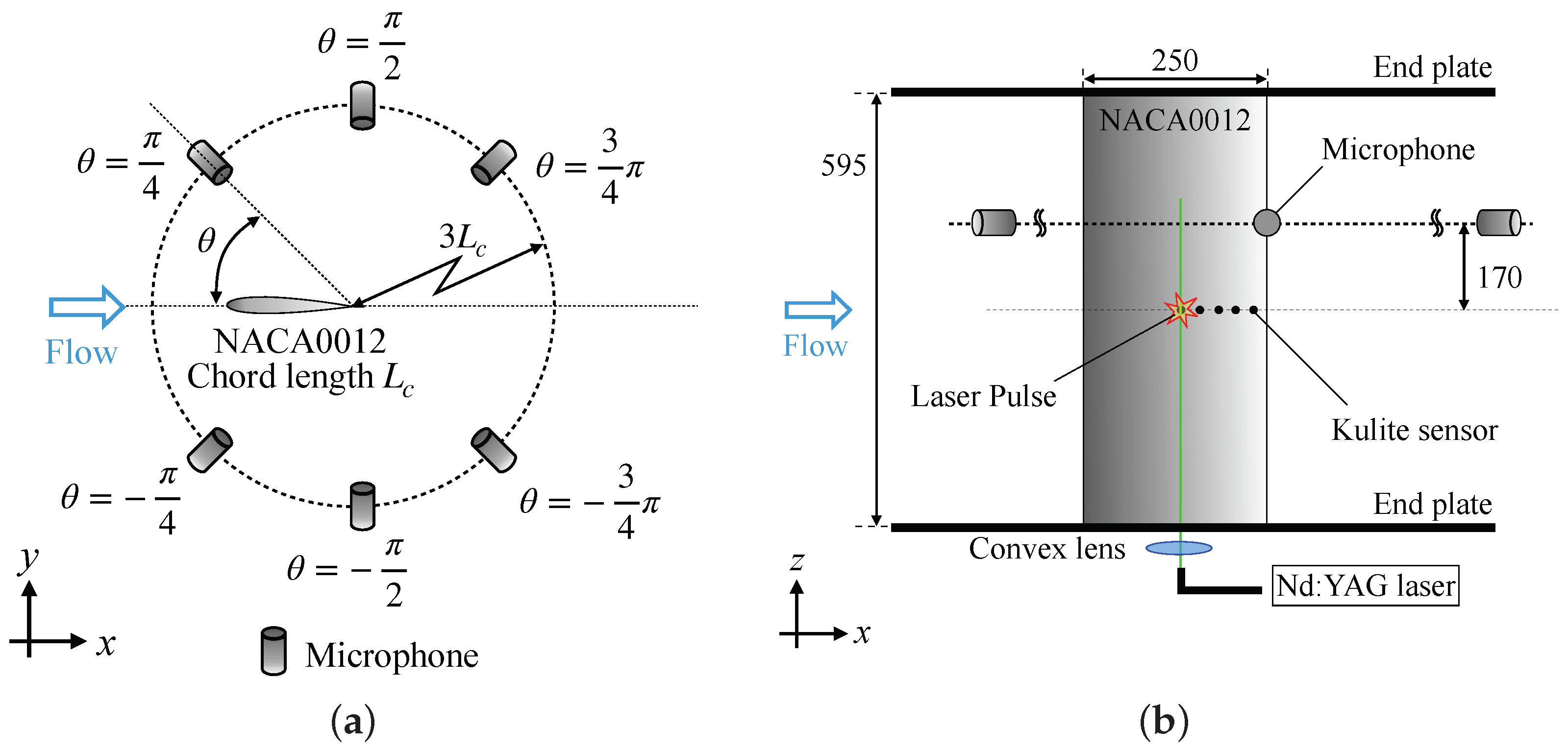
2.1. Experimental Setup
The wind tunnel experiments were conducted in the Low-Turbulence Wind Tunnel at the Chofu Aerospace Center of the Japan Aerospace Exploration Agency (JAXA), which is an open jet wind tunnel with a rectangular nozzle of a 650 mm × 550 mm cross-section. The nominal turbulence intensity, which is the root mean square value of the velocity fluctuations, at the nozzle is less than 0.05% of the free-stream velocity. The experimental setup is displayed in Figure 2.
Figure 2.
Experiment setup. (a) Side view; (b) Bottom view (dimensions in mm).
The wing model was a two-dimensional NACA0012 airfoil with a blunt trailing edge whose chord and span b are 250 mm and 595 mm, respectively. The model was made of aluminum alloy (Japanese Industrial Standards (JIS) A5052). End plates were installed at both spanwise ends of the wing to reduce the effect of the shear layer of airflow from the nozzle outlet. Five semiconductor pressure transducers (XCQ-093-5D, Kulite) were mounted on the wing at 50%, 60%, 70%, 80%, and 90% in the chord direction, which were located 50% in the span direction on the pressure surface.
An Nd:YAG laser (SAGA 230, Thales) was used as an actuator of the fluid flow. This laser has an output energy of 950 mJ/pulse at a wavelength of 532 nm, a pulse width of 6 ns, and a repetition rate of 10 Hz. Referring to previous studies [12,13,17], the focused laser beam was irradiated just outside of the velocity boundary layer, i.e., 3 mm away from the lower side surface and at 50% of the chord of the wing. A convex lens (SLB-30–500PM, SigmaKoki, focal length 500 mm) was used for laser focusing.
To measure the TE noise, we installed six microphones (Type 4958, Brüel & Kjær) 170 mm above the mid-span of the wing model on a circle of the radius , centered at the trailing edge. The pressure transducer and microphone were measured simultaneously at a sampling rate of 10 MHz using a digital oscilloscope (DL850, Yokogawa).
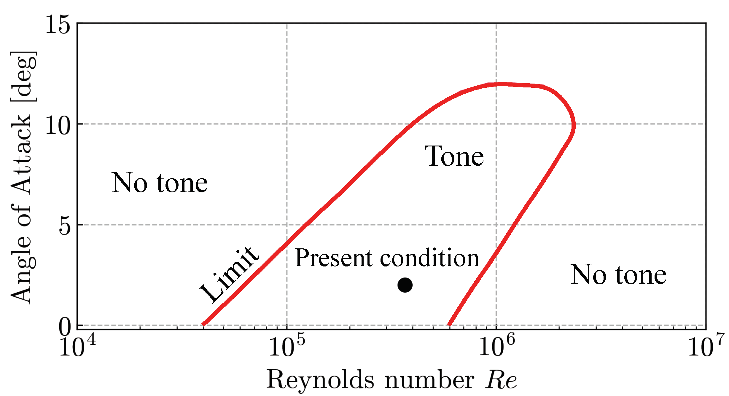
2.2. Experimental Conditions
In the wind tunnel experiments, the free stream was set at the velocity of m/s and the temperature of K, where the subscript ∞ denotes the uniform flow variables. The chord length-based Reynolds number was with the density and the visosity at the uniform flow. The angle of attack was fixed at . This flow condition is chosen using Lowson’s diagram [4] (Figure 3), which displays the Reynolds number and angle of attack region in which the tone noise phenomenon is expected. We assume that the external temperature has a small impact on the laser-driven control system since the temperature induced by the laser irradiation is much higher than the surrounding air [24]. Hence, we conducted the wind tunnel test at the standard room temperature. In this flow condition, the vortices on the lower airfoil surface were the main source of the TE noise [10].
Figure 3.
Predicted appearance of LBL instability noise by Lowson et al. [4]. The closed circle indicates the flow configurations employed for the present study.
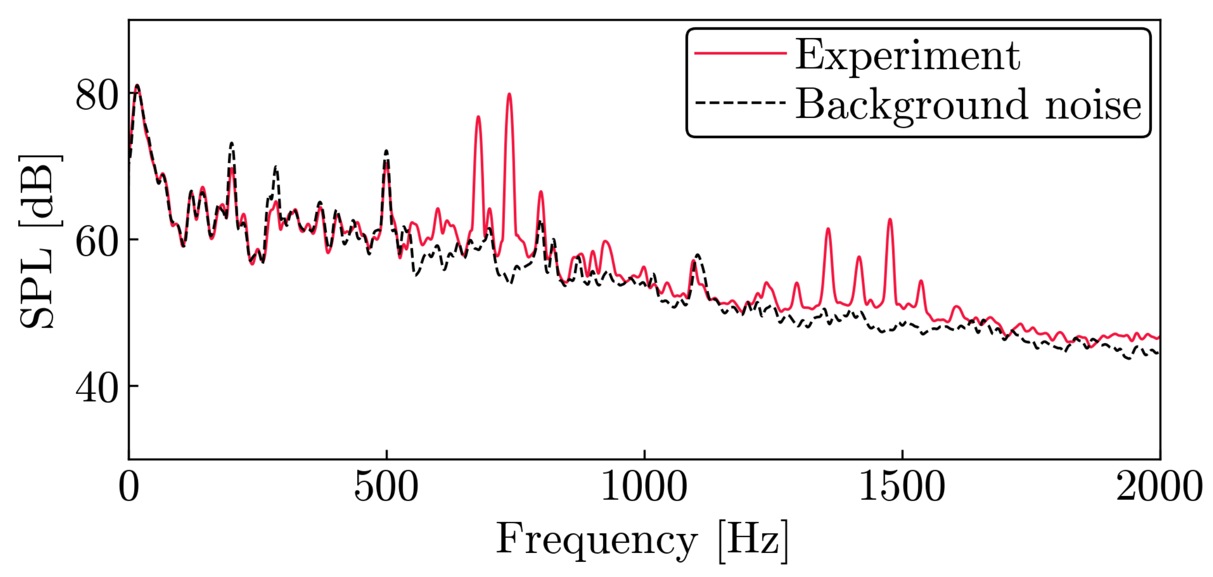
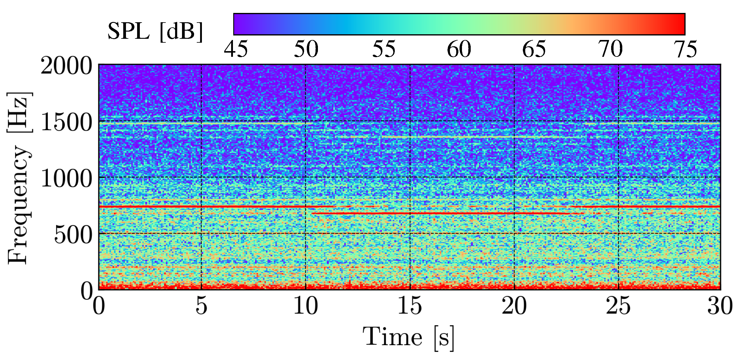
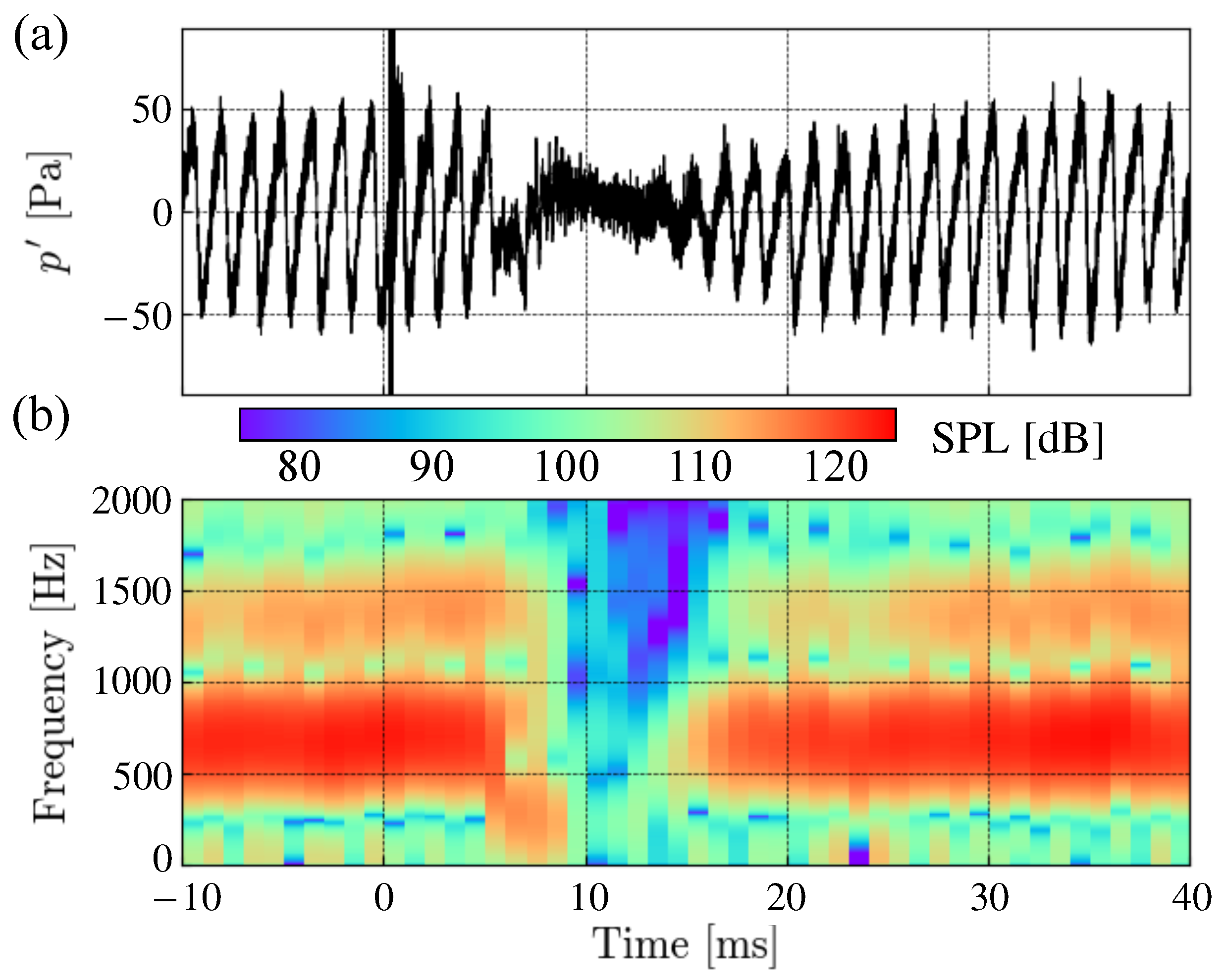
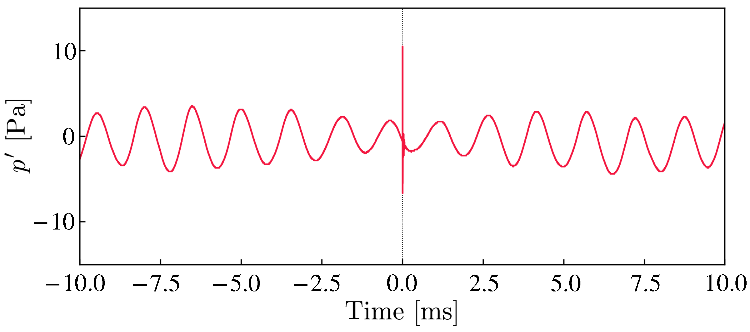
2.3. Experimental Results
First, the TE noise from the wing was observed without a laser deposition. Figure 4 shows the sound pressure level (SPL) of the pressure fluctuations () measured by the microphone located at . The bar indicates the time-averaged value. The SPL,
is calculated using the measured pressure. Here, is frequency resolution and is the reference pressure level Pa. PSD indicates the power spectral density function of the pressure fluctuations. The time series data were collected for 30.0 s with a recording rate of 50 kHz and were converted into the PSD by Welch’s method [25] together with a Hanning window. In the calculation, the time series was segmented into 200 sections, and Welch’s method was performed with a 50% overlap.
Figure 4.
Sound pressure level proved by a microphone at .
The red solid line in the Figure 4 shows the case where the wing model is installed, while the black dashed line shows the background noise without the model. The discrete tones associated with the trailing-edge noise are observed at the dominant frequencies of and 736 Hz, whose magnitudes are approximately 20 dB higher than the background noise level. Paterson et al. [2] suggested an empirical law for the dominant frequency, which is derived as , where and as the kinematic viscosity. The above relation can be deformed as . In the present condition, the primary peak is predicted as 613 Hz, which is roughly consistent with the wind tunnel result. The multiple peaks around the dominant frequency derive from the frequency modulation, as shown in the spectrogram in Figure 5. The complex interaction of the vortices on both sides of the airfoil causes the frequency modulation through the acoustic feedback loop [3].
Figure 5.
Spectrogram of pressure fluctuation proved by the microphone at .
Next, let us explain the effect of the laser deposition on the boundary layer over the airfoil. We examined the pressure fluctuations on the lower surface because the velocity fluctuations on the lower airfoil surface were the main noise source in the current flow condition [10]. The surface pressure fluctuations were correlated with the intensity of the velocity fluctuations by the TS wave and vortices, which are the source of the TE noise illustrated in Figure 1.
The surface pressure fluctuations probed at (90% chord position) on the lower surface are presented in Figure 6a. The time indicates the time when the pulsed laser was irradiated. Figure 6b shows the spectrogram calculated with the time window of 4 ms. The time series data were collected for 0.2 s with a recording rate of 10 MHz and were converted into the PSD by Welch’s method [25] together with a Hanning window. In the calculation, the time series was segmented into 50 sections, and Welch’s method was performed with a 75% overlap. The periodic fluctuation with a frequency of about 700 Hz corresponds to the convection of the velocity fluctuations on the airfoil’s surface.
Figure 6.
(a) Unsteady surface pressure fluctuation measured at (90% chord position). (b) Spectrogram of (a). The width of the time window is 4 ms.
Figure 6 indicates that the periodic pressure fluctuation observed before the irradiation of the pulsed laser is reduced by the energy deposition of the disturbance near the boundary layer. Once the pulsed laser is applied at , the pressure waves generated by the air breakdown cause strong pressure fluctuations at the transducer. The peak pressure value was 274 Pa for the maximum and Pa for the minimum. The fluctuation amplitude decreases after 6 ms of the deposition. The amplitude slightly recovers at time and remains small until . The signal then gradually recovers its amplitude to the original state.
The frequency–time diagram in Figure 6b shows that the fluctuation is suppressed not only for the dominant frequency of 680 Hz but also for the overall frequencies between 6.0 ms and 16.0 ms. We experimentally confirmed that the pulsed laser could reduce the pressure fluctuation due to the TE noise within a certain time range by an energy deposition just outside of the boundary layer.
3. Numerical Setup for the Simulation
For analyzing the mechanism of the TE noise control by a pulsed laser, unsteady flows around the NACA0012 wing were simulated based on the wind tunnel experiments described in Section 2. This section explains the numerical setup for the simulations and a numerical model of the pulsed laser.
3.1. Governing Equations
We considered the governing equation of the fluid flow in its three-dimensional and compressible form:
The conservative variable is defined as , where are the density, streamwise velocity, cross-stream velocity, spanwise velocity and total energy per unit mass, respectively. denotes the source term due to the energy deposition as described in Section 3.2. and are the inviscid flux and viscous flux, respectively. Details of the governing equations are provided in Appendix A.
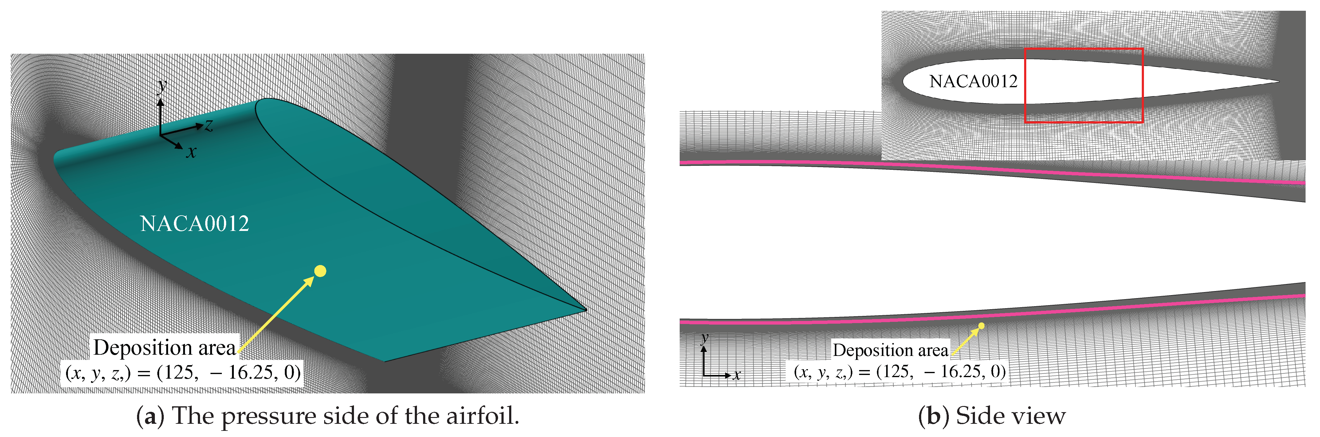
3.2. Modeling of Energy Deposition
The source term on the right-hand side of Equation (2) was formulated as a model of the energy deposition by the pulsed laser:
where is defined as with the input energy per unit mass and the volume of the deposited energy source . Assuming that the beam profile possesses a Gaussian distribution, the spatial distribution of the power cross-section is given by
where r and are the distance from the laser’s center and the laser’s radius, respectively. is the peak intensity of the Gaussian beam per unit of time. is the set function for determining the energy deposition. We assumed that the energy per unit of time in the radius of was equivalent to the deposited energy .
Thus, is written as
The deposited energy per unit time is related to the pressure impulse as
where , , and are the energy application time, the ratio of specific heats, and the density, respectively. The pressure impulse can be evaluated experimentally from the signal of the pressure transducer below the laser’s deposition point. In addition, in Equation (3) is the set function for determining the energy deposition in time:
where indicates the pulse interval time.
Tagawa et al. [26] reported that the focused laser irradiation generated a few millimeters-long row of plasma beads, causing multiple spherical shock waves along with the beamline. Figure 7 shows a model of the plasma beads in this study. The focal spots were equally spaced with a pitch of within the length . The timing of the energy deposition was assumed to be the same for all spots. We examined the pressure fluctuations at (50% chord position) on the pressure side surface in Figure 8 to confirm that the pulse is introduced in the flow at . We observed a strong pressure fluctuation by the energy deposition.
Figure 7.
Model of plasma beads.
Figure 8.
Pressure fluctuations measured at mm (50% chord position) on the pressure side surface.
3.3. Numerical Method and Conditions
The government equation with the pulsed laser model was solved by FaSTAR (FAST Aerodynamic Routines), a finite volume method-based compressible flow solver developed at JAXA [27]. For the turbulent flow simulation, we employed the implicit large eddy simulation (ILES), a high-fidelity method of computational fluid dynamics (CFD). Previous research [28] has confirmed that the flow simulation using the ILES method successfully captures the key physics of the TE noise phenomenon, including the TS wave growth and consequent forming to the turbulent vortex that causes the tonal noise. A detail of the numerical method is shown in Appendix B. We define the coordinate origin to be at the airfoil leading edge. The flow condition of the simulation was the same as the wind tunnel experiment.
In this study, we considered two pulse conditions with different , as summarized in Table 1. The “Narrow” case has the same length of the pulses chain as the wind tunnel test, whereas the “Wide” case has a longer length. Calculations were performed in two sets of , , and listed in Table 1. In both cases, the pressure impulse and the energy application time were equal. The center of the chain of plasma beads was set as as shown Figure 9. The two parameters and in Equation (7) were determined as and μs. These parameters were determined to fit the pressure fluctuation in the experiment shown in Figure 6.
Table 1.
The condition of energy deposition.
Figure 9.
Deposition area. (a) The center of the string of plasma beads was set as . The magenta line in (b) indicates , which is the boundary layer.
4. Numerical Results and Discussion
This section presents the numerical results from the simulations described in Section 3 and discusses how the pulsed laser suppresses the trailing-edge noise. We also consider the two focal spot arrangements in Table 1.
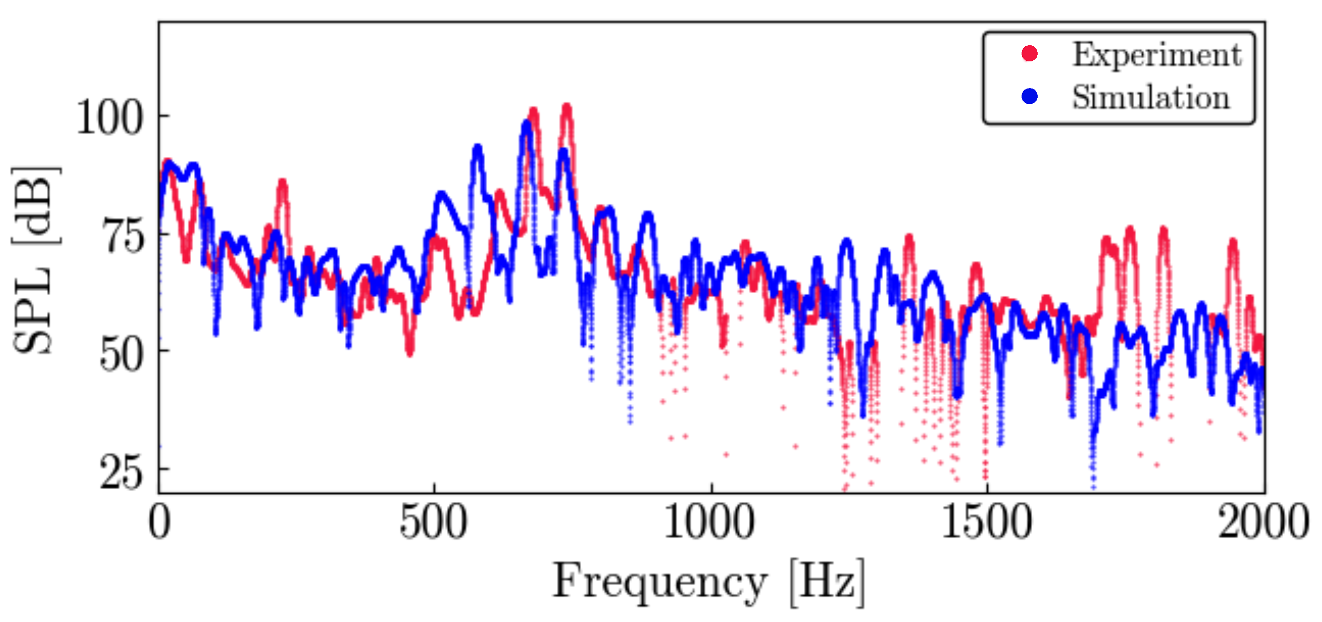
4.1. Validation of the Present Computation
First, we validated the numerical simulation by examining the pressure fields without the energy deposition. Figure 10 shows an instantaneous pressure fluctuation at . The dipolar distribution about the surface indicates that the present computation properly simulates the target acoustic phenomenon emitted from the trailing edge. We also compare the pressure fluctuation on the airfoil’s surface with the wind tunnel data in Section 2. The SPL probed at mm (80% chord position) on the pressure surface in Figure 11 indicates good agreements between the present computation and the experimental data. The figure shows the typical characteristic frequencies associated with the trailing-edge noise. The dominant peak frequency in the numerical simulations is Hz, close to the experimental value of 677 Hz. The multiple peaks around the dominant frequency are also observed in the wind tunnel test and are reported in several previous studies [3,12]. Some peaks between 1700 Hz and 2000 Hz of the experiment in Figure 11 are caused by measurement noise because they have the same SPL level even if observed at another transducer. These results confirm that the present calculations capture the essential features of the flow field with the TE noise in the experiment.
Figure 10.
Instantaneous pressure fluctuations at .
Figure 11.
Sound pressure level probed at mm (corresponding to 80% chord position) on the pressure side surface.
4.2. Energy Deposition near the Boundary Layer
Let us discuss the cases with energy depositions to investigate the control effect of the TE noise. We assume that the energy deposition takes place at . Both cases in Table 1 are considered in this section. Figure 12 shows the time history of the pressure fluctuations measured at mm, which simulate the microphone at in the wind tunnel test. The figure indicates that the pressure fluctuations at the microphone retain their amplitudes until ms in both cases. In the Narrow case, which simulates the laser pulse in the wind tunnel test, the amplitude reduces in the period from to ms. After ms, the amplitude gradually recovers. In the case of Wide, the amplitude decreases after ms, and the decrease continues during the period in this figure. The result suggests that the Wide case is more effective in reducing TE noise than the Narrow case.
Figure 12.
Pressure fluctuations measured at which simulate a microphone at in wind tunnel test. (a) Narrow; (b) Wide.
Next, we examine the pressure fluctuations on the airfoil wall. As we explained in Section 2, the surface pressure fluctuations on the lower airfoil surface are correlated with the intensity of the velocity fluctuations by the TS wave and the vortices. Figure 13 shows the time history of the surface pressure fluctuations measured at (corresponding to 90% chord position) on the lower side surface around the energy deposition time. We note that the amplitudes of these fluctuations are smaller than the experimental result in Figure 6. The discrepancies might come from the difference in the separation bubble sizes, which affects the amplitude of the pressure fluctuations near the trailing edge [3,7]. However, considering that the current computation simulates the qualitative behavior of the pressure response after laser irradiation (see Figure 6a and Figure 13a), the presented result provides the key physics of the targeted wind tunnel test. These fluctuations in the surface pressure are closely related to the amplitudes of the TE noise detected by microphones shown in Figure 12. For example, in the Narrow case, the pressure fluctuation retains its amplitude until . Following the large amplitude of pressure fluctuations from ms to 20 ms, a decrease in the amplitude is observed from ms to 40 ms. Finally, the pressure fluctuations recover to the same state as before the pulsed laser irradiation.
Figure 13.
Pressure fluctuations measured at (90% chord position) on the pressure side surface. (a) Narrow; (b) Wide.
Here we divide this process into four phases, as shown in Figure 13. The duration when the pressure fluctuations correspond to the basic state of the TE noise is called phase(I). The period of time during which the amplitude temporarily increases due to the application of the laser energy is called phase (II). The subsequent period of decreasing the amplitude is called phase (III). The final recovery to the basic state is called (IV). It should be emphasized that these phases are equivalent to those observed in the experiment shown in Figure 6.
Phases (I), (II), and (III) are also observed in the Wide case. Only phase (IV) is unclear since the amplitude reduction continues for extended periods.
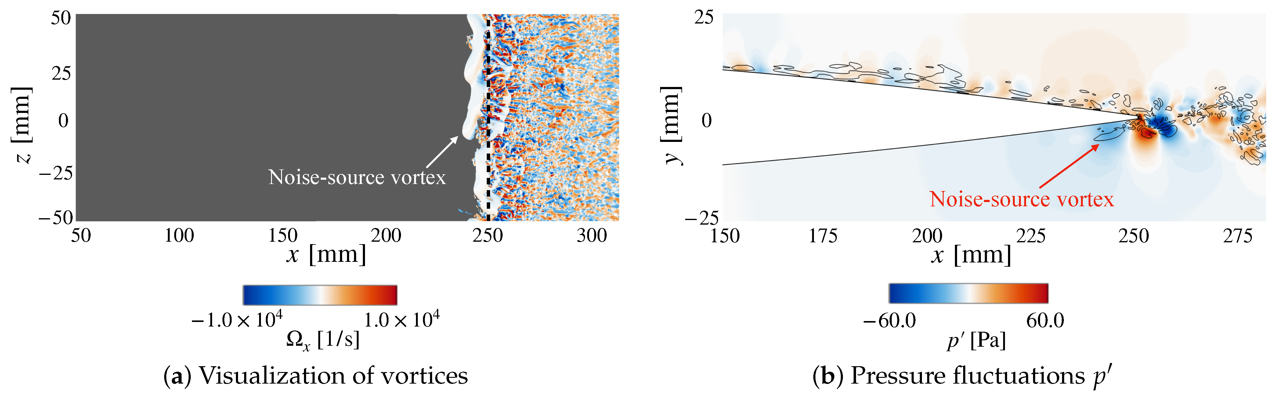
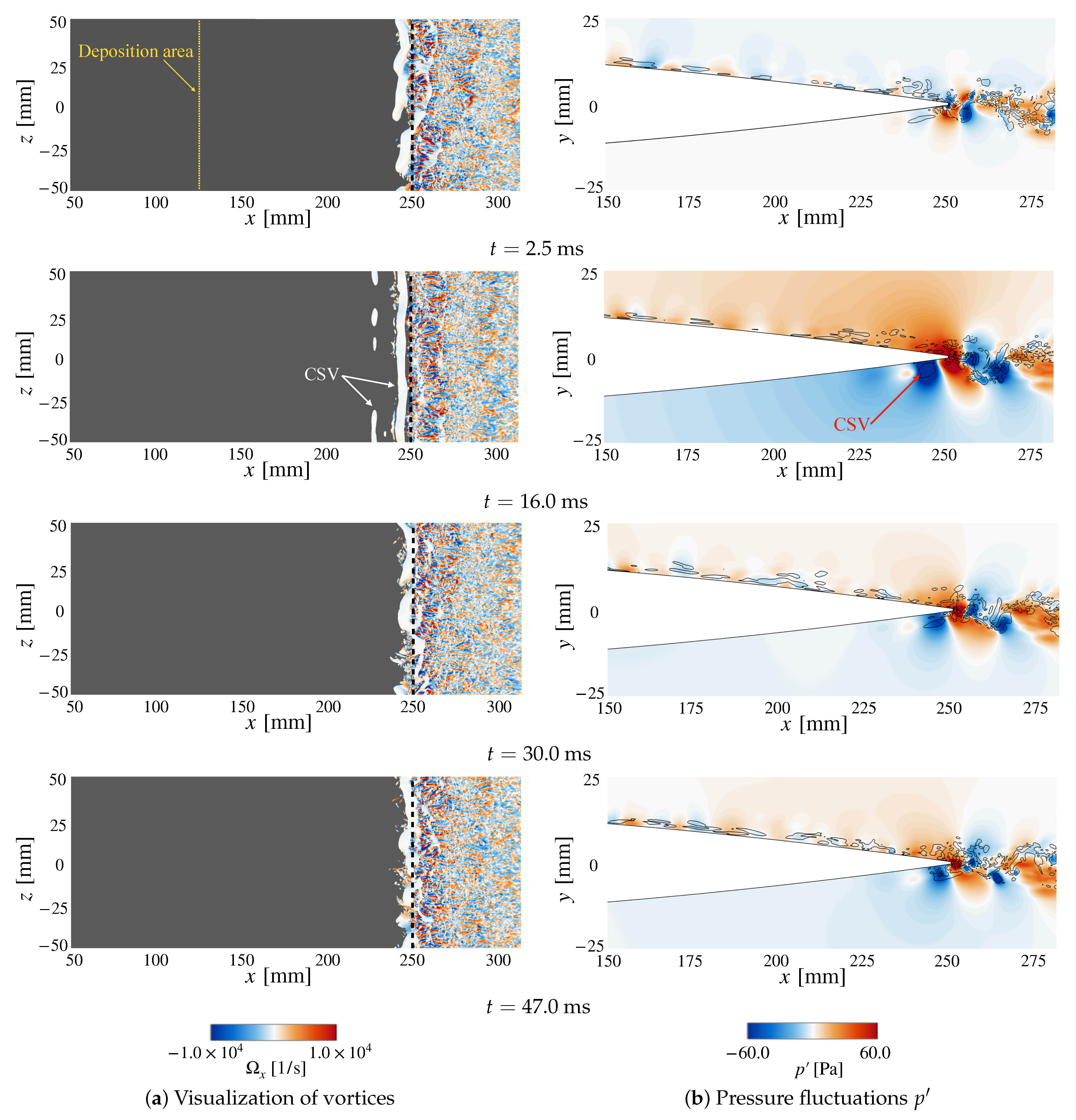
4.3. Dynamics of Vortices near the Trailing Edge
The mechanism of the TE noise generation implies that the energy deposition should affect the vortices on the airfoil’s surface, which in turn suppresses the TE noise. Therefore, this section investigates the vortex dynamics for both cases in Table 1 and presents a detail of the TE noise reduction mechanism. We examine instantaneous iso-surfaces of Q-criterion [29] defined as − , where and are the vorticity tensor and the strain rate tensor, respectively. The Q criterion is an often-used quantity in fluid dynamics to visualize vortices in the fluid flow. Figure 14, Figure 15 and Figure 16 show the flow field before the energy deposition, in the Narrow case and the Wide case, respectively. A relatively large vortex with a uniform structure in the spanwise direction is visualized in Figure 14, indicating that this is the source of trailing-edge noise. Here, we analyze how this vortex changes by the deposition of the pulsed laser. The following discussion proceeds from phase (II) to (IV) presented in the previous section.
Figure 14.
A visualization of the instantaneous flow field just before the energy deposition at ms. The figures show (a) vortices by iso-surfaces of Q-criterion () and (b) pressure fluctuations , respectively. The iso-surfaces are colored by x-wise vorticity . The black-dashed line in (a) indicates the trailing edge of the airfoil. The pressure field also shows contour lines of .
Figure 15.
Time series of instantaneous flow field from to ms for the Narrow case. The definitions of iso-surfaces and contours are the same as in Figure 14. The figure also shows the deposition area with the yellow-dashed line.
Figure 16.
Time series of instantaneous flow field from to ms for the Wide case. The definitions of iso-surfaces and contours are the same as in Figure 14. The figure also shows the deposition area with the yellow-dashed line.
The pressure fluctuation at (corresponding to a 90% chord position) in Figure 13 shows the pressure increase at , indicating that the induced vortex by the energy deposition reaches the probe position at phase (II). Figure 15 and Figure 16 at visualize the vortices propagating from the pulse location and passing through the trailing edge for both cases. The pulse-induced vortices have pretty different shapes depending on the pulse condition. In the Narrow case, the vortex has an arc-like shape centered at the pulse position, and we call it an arcuate spread vortex (ASV) hereafter. The vortex in the Wide case is relatively uniform in the spanwise direction, and we call this vortex a cylindrical spread vortex (CSV).
We emphasize that the ASV and CSV induced by the pulsed laser have quite different properties from the noise-source vortices. Figure 17 shows the time histories of the velocity fluctuation that reflect the time development of the ASV and CSV. The laser-induced fluctuations appear around ms with an interval of ms, corresponding to a frequency of 595 Hz. Reminding that the trailing-edge noise and the source vortices have a dominant frequency of 663 Hz, the time histories indicate that the laser irradiation excites an unstable mode different from the mode of the noise source.
Figure 17.
The figures show stream-wise velocity measured at (corresponding to 90% chord position) on the lower side surface.
The visualizations at ms and ms in Figure 15 and Figure 16 show the vortex dynamics related to phases (III) and (IV) in Figure 13. In the Narrow case, as shown in Figure 15, the visualization of the vortices at ms shows that the ASV sweeps out the source vortices of TE noise observed in Figure 14. The source vortices are then reconstructed at ms, corresponding to the amplitude recovering at phase (IV) in Figure 13. These results indicate that the disappearance of the source vortices by the ASV leads to a reduction in the noise.
In the Wide case, the CSV interacts with the source vortices at ms. The major difference from the Narrow case is that the CSV does not sweep out the source vortices completely but rather disturbs their spanwise uniformity. The non-uniformity of the vortices would induce incoherent sound waves in the spanwise direction. The TE noise is attenuated when the waves interfere with each other. Figure 13 indicates that it takes longer to recover the uniformity of the vortices than to reconstruct the source vortices in the Narrow case.
4.4. Aerodynamic Characteristics
This section investigates the lift-drag characteristics for both cases in Table 1. We examine the time variation in the drag and lift coefficients in Figure 18 and Figure 19, respectively. The drag history in Figure 18 indicates that there was a reduction of 21% for the Narrow and 30% for the Wide case. Notably, the significant increase in the drag force does not occur when the laser irradiates. However, the lift history in Figure 19 shows that the lift coefficients also decrease by 16% for the Narrow case and 27% for the Wide case. The lift decrease is caused by the detachment of the vortex generated by a laser irradiation.
Figure 18.
Time history of the drag coefficient . (a) Narrow; (b) Wide.
Figure 19.
Time history of the lift coefficient . (a) Narrow; (b) Wide.
4.5. Implementation of the Laser Actuator for Actual Aircraft
Finally, we present our future plan regarding how the laser actuator in this study would be installed in an actual aircraft, as schematically explained in Figure 20. The figure illustrates that the laser irradiation from the wing root focuses on the airfoil’s surface to control the flow field. In the illustration, we take advantage of the wing tip as a laser damper to cut off the laser. We believe the presented actuator could provide one possible option to control aircraft noise.
Figure 20.
Laser actuator for actual aircraft.
5. Conclusions
In this paper, we employed the laser actuator to reduce the TE noise from the airfoil. We conducted experimental and numerical research to examine the noise control effect and investigate the details of the noise control mechanism. In the numerical investigation, we considered two energy deposition area shapes: the Narrow and Wide cases. The principal findings in the present paper are summarized as follows:
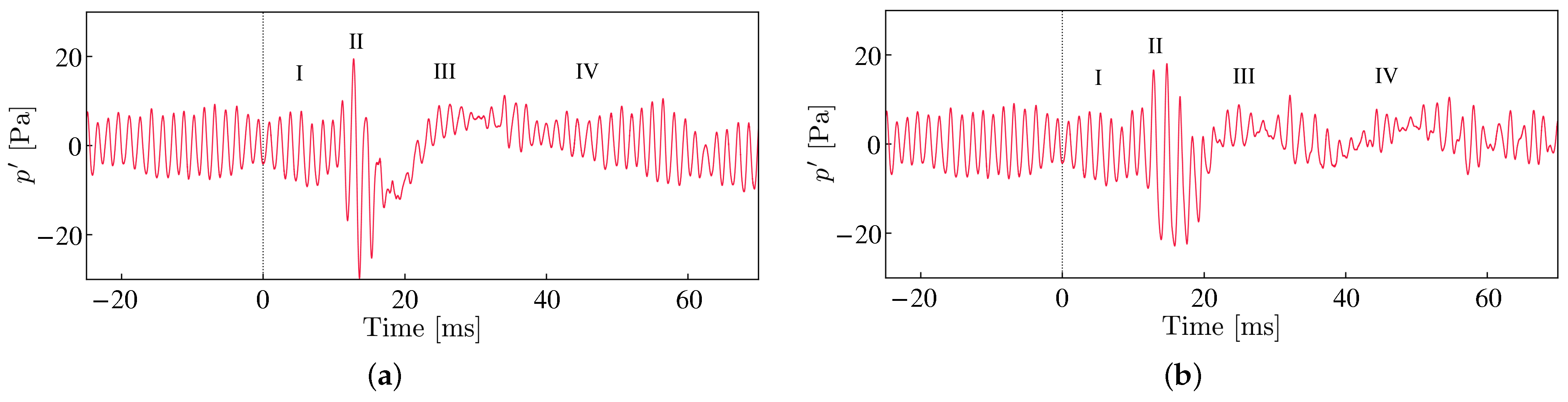
- The experimental result indicates that a laser irradiation can reduce the intensity of the surface pressure fluctuations that are the source of the TE noise.
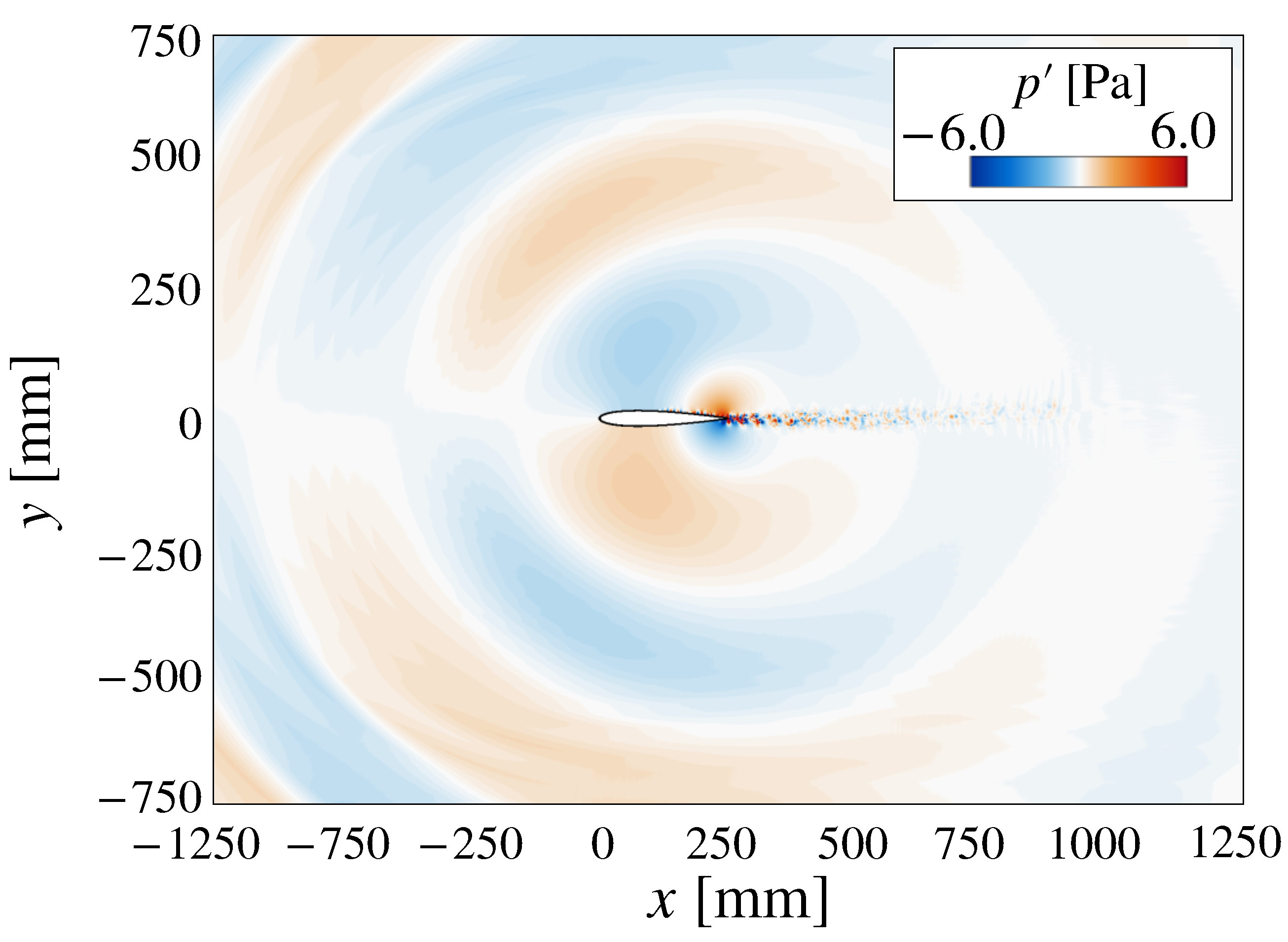
- The numerical investigations suggest that a laser irradiation induces a characteristic vortex depending on the energy deposition area shapes. In the Narrow case, the energy deposition to the narrow domain introduces vortices with a curved shape named an accurate spread vortex (ASV). In contrast, the relatively spanwise uniform vortex called a cylindrical spread vortex (CSV) is observed in the Wide case. The ASV swept out the source vortices of the TE noise and broke the acoustic feedback mechanism that sustains the TE noise. The CSV disturbs the spanwise uniformity of the noise-source vortices, resulting in a spanwise-incoherent noise radiation, which might cancel out each other.
- The Wide case is more effective in reducing the source vortex intensity if the amount of energy decompositions is the same as the Narrow case.
Author Contributions
Conceptualization, K.O., Y.K., M.I., K.N. and M.K.; methodology, K.O., Y.K., M.K., K.N. and M.I.; experiment, K.O., M.I., K.K. and K.N.; software, K.O.; data analysis, K.O.; writing—original draft preparation, K.O.; writing—review and editing, Y.K. and M.K.; supervision, M.K.; project administration, M.K.; funding acquisition, M.K. All authors have read and agreed to the published version of the manuscript.
Funding
This research was funded by JSPS KAKENHI under Grant numbers 20K21043 and 22H01396.
Institutional Review Board Statement
Not applicable.
Informed Consent Statement
Not applicable.
Data Availability Statement
Not applicable.
Acknowledgments
The numerical simulations in this research were performed at JAXA Supercomputer System generation 3 (JSS3). The authors would like to thank Koichi Suzuki and Takashi Yajima, and all the members of the Low-Turbulence Wind Tunnel for their technical support for the wind tunnel test.
Conflicts of Interest
The authors declare no conflict of interest. The funders had no role in the design of the study; in the collection, analyses, or interpretation of data; in the writing of the manuscript; or in the decision to publish the results.
Abbreviations
The following abbreviations are used in this manuscript:
| ILES | Implicit large-eddy simulation |
| SPL | Sound pressure level |
| PSD | Power spectral density |
| ASV | Arcuate spread vortex |
| CSV | Cylindrical spread vortex |
Appendix A. Detail of Governing Equations
In this section, we explain the details on the governing equation of FaSTAR. We consider the three-dimensional compressible form of the governing equation:
The conservative variables are defined as , where are the density, streamwise velocity, cross-stream velocity, spanwise velocity, and total energy per unit mass, respectively. The superscript T denotes the matrix transpose. Inviscid flux and viscous flux are defined as
and
where , , and are the unit vertor and p is the pressure. The viscous components of the momentum and energy fluxes are given by
where and T are the thermal conductivity and temperature, respectively. The dynamic viscosity is calculated by Sutherland’s law.
Here, C is an effective temperature called the Sutherland constant. The subscript indicates the reference variable. We employ the equation of state for closure.
Here, R is the gas constant.
Appendix B. Details of Numerical Method
In this appendix, we provide the details of the numerical method in this study. The numerical scheme for estimating the inviscid flux in the Equation (A2) is based on the KEP (Kinetic Energy Preserving) scheme [30,31,32]. The gradient, which is needed for evaluating the viscous flux, is evaluated by the Green–Gauss-based weighted least square method (GLSQ) [33]. The time integration is carried out by a second-order implicit LU-SGS method [34]. The physical time step is set as , which satisfies the Courant–Friedrichs–Lewy (CFL) condition throughout the computational domain.
We used a hexahedral grid with C-type topology for a numerical simulation, as shown in Figure A1. The computational domain has an extent of , , and which is sufficiently large to capture aeroacoustics. The computational grid is fine enough with grid points in the streamwise, wall-normal, and spanwise directions which are 600 nodes, 228 nodes, and 200 nodes, respectively. The total number of numerical cells is approximately . The grid spacings are set to meet the conditions of , , and at , where the superscript + indicates the wall unit. Furthermore, we adopted and the first wall cells at the trailing edge for both sides of the airfoil. The spanwise grid spacing is uniformly set as . The grid resolutions in the present study are fine enough to simulate the boundary layer transition on the suction side of the airfoil. For the far-field boundary, numerical damping is applied to avoid the reflection of outgoing waves. The free-stream condition is prescribed at the far-field boundary, whereas the no-slip adiabatic condition is prescribed over the airfoil. A periodic boundary condition is set over the boundary of spanwise directions.
Figure A1.
Numerical grid for the simulations. (a) Whole area; (b) Near the airfoil.
Appendix C. Nomenclature
Table A1.
Physical quantity symbols and units in this paper.
Table A1.
Physical quantity symbols and units in this paper.
| Symbol | Unit | Parameter Description |
|---|---|---|
| Coordinate values | ||
| x, y, z wise velocity | ||
| Chord length | ||
| Angle of attack | ||
| - | Mach number | |
| - | Chord length-based Reynolds number | |
| Density | ||
| e | Total energy per unit mass | |
| p | Pa | Pressure |
| T | K | Temperature |
| Dynamics viscosity | ||
| - | Specific heat ratio | |
| V | Volume | |
| - | Inviscid and viscous flux of the Navier–Stokes equation | |
| - | Source term of the energy application by pulsed laser | |
| Input energy per unit mass and time | ||
| Peak intensity of Gaussian beam per unit mass and time | ||
| Deposited energy per unit mass and time | ||
| s | Pulse duration time | |
| s | Pulse interval time | |
| Pressure impulse | ||
| r | m | Distance from the laser’ center |
| m | Laser’s radius | |
| m | Pitch of the focal spots | |
| m | Length of the plasma beads | |
| t | s | Time |
| f | Hz | Frequency |
| Vorticity | ||
| Q | Q-criterion, a second invariant of the strain rate tensor | |
| ∞ | - | Uniform flow value |
| - | Time-averaged value | |
| + | - | Wall unit value |
References
- Yamamoto, K.; Hayama, K.; Kumada, T.; Hayashi, K. A flight demonstration for airframe noise reduction technology. CEAS Aeronaut. J. 2019, 10, 77–92. [Google Scholar] [CrossRef]
- Paterson, R.W.; Vogt, P.G.; Fink, M.R.; Munch, C.L. Vortex Noise of Isolated Airfoils. J. Aircr. 1973, 10, 296–302. [Google Scholar] [CrossRef]
- Desquesnes, G.; Terracol, M.; Sagaut, P. Numerical investigation of the tone noise mechanism over laminar airfoils. J. Fluid Mech. 2007, 591, 155–182. [Google Scholar] [CrossRef]
- Lowson, M.; Fiddes, S.; Nash, E. Laminar boundary layer aero-acoustic instabilities. In Proceedings of the 32nd Aerospace Sciences Meeting and Exhibit, Reno, NV, USA, 10–13 January 1994. [Google Scholar] [CrossRef]
- Brooks, T.F.; Pope, D.S.; Marcolini, M.A. Airfoil Self-noise and Prediction. Technical Report. 1989. Available online: https://ntrs.nasa.gov/citations/19890016302 (accessed on 28 December 2022).
- Arbey, H.; Bataille, J. Noise generated by airfoil profiles placed in a uniform laminar flow. J. Fluid Mech. 1983, 134, 33–47. [Google Scholar] [CrossRef]
- Nash, E.C.; Lowson, M.V.; McALPINE, A. Boundary-layer instability noise on aerofoils. J. Fluid Mech. 1999, 382, 27–61. [Google Scholar] [CrossRef]
- Pröbsting, S.; Yarusevych, S. Laminar separation bubble development on an airfoil emitting tonal noise. J. Fluid Mech. 2015, 780, 167–191. [Google Scholar] [CrossRef]
- Nakano, T.; Fujisawa, N.; Lee, S. Measurement of tonal-noise characteristics and periodic flow structure around NACA0018 airfoil. Exp. Fluids 2006, 40, 482–490. [Google Scholar] [CrossRef]
- Noda, T.; Nakakita, K.; Wakahara, M.; Kameda, M. Detection of small-amplitude periodic surface pressure fluctuation by pressure-sensitive paint measurements using frequency-domain methods. Exp. Fluids 2018, 59, 94. [Google Scholar] [CrossRef]
- Taira, K.; Colonius, T. Three-dimensional flows around low-aspect-ratio flat-plate wings at low Reynolds numbers. J. Fluid Mech. 2009, 623, 187–207. [Google Scholar] [CrossRef]
- Fosas de Pando, M.; Schmid, P.J.; Sipp, D. A global analysis of tonal noise in flows around aerofoils. J. Fluid Mech. 2014, 754, 5–38. [Google Scholar] [CrossRef]
- Fosas de Pando, M.; Schmid, P.J.; Sipp, D. On the receptivity of aerofoil tonal noise: An adjoint analysis. J. Fluid Mech. 2017, 812, 771–791. [Google Scholar] [CrossRef]
- Ricciardi, T.R.; Wolf, W.R.; Taira, K. Transition, intermittency and phase interference effects in airfoil secondary tones and acoustic feedback loop. J. Fluid Mech. 2022, 937, A23. [Google Scholar] [CrossRef]
- Goldin, N.; King, R.; Pätzold, A.; Nitsche, W.; Haller, D.; Woias, P. Laminar flow control with distributed surface actuation: Damping Tollmien-Schlichting waves with active surface displacement. Exp. Fluids 2013, 54, 1478. [Google Scholar] [CrossRef]
- Wylie, J.D.B.; Mishra, S.; Amitay, M. Tollmien–Schlichting Wave Control on an Airfoil Using Dynamic Surface Modification. AIAA J. 2021, 59, 2890–2900. [Google Scholar] [CrossRef]
- Inasawa, A.; Ninomiya, C.; Asai, M. Suppression of Tonal Trailing-Edge Noise From an Airfoil Using a Plasma Actuator. AIAA J. 2013, 51, 1695–1702. [Google Scholar] [CrossRef]
- Simon, B.; Markus, D.; Tropea, C.; Grundmann, S. Cancellation of Tollmien-Schlichting Waves in Direct Vicinity of a Plasma Actuator. AIAA J. 2018, 56, 1760–1769. [Google Scholar] [CrossRef]
- Simon, B.; Fabbiane, N.; Nemitz, T.; Bagheri, S.; Henningson, D.S.; Grundmann, S. In-flight active wave cancelation with delayed-x-LMS control algorithm in a laminar boundary layer. Exp. Fluids 2016, 57, 160. [Google Scholar] [CrossRef]
- Déda, T.C.; Wolf, W.R. Extremum Seeking Control Applied to Airfoil Trailing-Edge Noise Suppression. AIAA J. 2022, 60, 823–843. [Google Scholar] [CrossRef]
- Tang, H.; Lei, Y.; Fu, Y. Noise Reduction Mechanisms of an Airfoil with Trailing Edge Serrations at Low Mach Number. Appl. Sci. 2019, 9, 3784. [Google Scholar] [CrossRef]
- Kremeyer, K.P. Energy Deposition II: Physical Mechanisms Underlying Techniques to Achieve High-Speed Flow Control. In Proceedings of the International Space Planes and Hypersonic Systems and Technologies Conferences, Glasgow, UK, 6–9 July 2015. [Google Scholar] [CrossRef]
- Kim, J.H.; Matsuda, A.; Sakai, T.; Sasoh, A. Wave Drag Reduction with Acting Spike Induced by Laser-Pulse Energy Depositions. AIAA J. 2011, 49, 2076–2078. [Google Scholar] [CrossRef]
- Bright, A.; Tichenor, N.; Kremeyer, K.; Wlezien, R. Boundary-Layer Separation Control Using Laser-Induced Air Breakdown. AIAA J. 2018, 56, 1472–1482. [Google Scholar] [CrossRef]
- Welch, P. The use of fast Fourier transform for the estimation of power spectra: A method based on time averaging over short, modified periodograms. IEEE Trans. Audio Electroacoust. 1967, 15, 70–73. [Google Scholar] [CrossRef]
- Tagawa, Y.; Yamamoto, S.; Hayasaka, K.; Kameda, M. On pressure impulse of a laser-induced underwater shock wave. J. Fluid Mech. 2016, 808, 5–18. [Google Scholar] [CrossRef]
- Hashimoto, A.; Murakami, K.; Aoyama, T.; Ishiko, K.; Hishida, M.; Sakashita, M.; Lahur, P. Toward the Fastest Unstructured CFD Code ‘FaSTAR’. In Proceedings of the 50th AIAA Aerospace Sciences Meetings, Nashville, TN, USA, 9–12 January 2012. [Google Scholar] [CrossRef]
- Ricciardi, T.R.; Wolf, W.; Taira, K. Compressibility Effects in Airfoil Secondary Tones. In Proceedings of the AIAA Scitech 2021 Forum, Virtual Event, 11–15, 19–21 January 2021. [Google Scholar] [CrossRef]
- Hunt, J.C.R. Eddies, Streams and Convergence Zones in Turbulent Flows. In Proceeding of the Summer Program in Center for Turbulence Research, NASA Ames, Stanford, CA, USA, 27 June–22 July 1988; pp. 193–207. [Google Scholar]
- Jameson, A. The Construction of Discretely Conservative Finite Volume Schemes that Also Globally Conserve Energy or Entropy. J. Sci. Comput. 2008, 34, 152–187. [Google Scholar] [CrossRef]
- Jameson, A. Formulation of Kinetic Energy Preserving Conservative Schemes for Gas Dynamics and Direct Numerical Simulation of One-Dimensional Viscous Compressible Flow in a Shock Tube Using Entropy and Kinetic Energy Preserving Schemes. J. Sci. Comput. 2008, 34, 188–208. [Google Scholar] [CrossRef]
- Kojima, Y.; Hashimoto, A. Embedded Large Eddy Simulation of Transonic Flow over an OAT15A Airfoil. In Proceedings of the AIAA SciTech Forum 2022, San Diego, CA, USA, 3–7 January 2022. [Google Scholar] [CrossRef]
- Shima, E.; Kitamura, K.; Haga, T. Green–Gauss/Weighted-Least-Squares Hybrid Gradient Reconstruction for Arbitrary Polyhedra Unstructured Grids. AIAA J. 2013, 51, 2740–2747. [Google Scholar] [CrossRef]
- Yoon, S.; Jameson, A. Lower-upper Symmetric-Gauss-Seidel method for the Euler and Navier–Stokes equations. AIAA J. 1988, 26, 1025–1026. [Google Scholar] [CrossRef]
Disclaimer/Publisher’s Note: The statements, opinions and data contained in all publications are solely those of the individual author(s) and contributor(s) and not of MDPI and/or the editor(s). MDPI and/or the editor(s) disclaim responsibility for any injury to people or property resulting from any ideas, methods, instructions or products referred to in the content. |
© 2023 by the authors. Licensee MDPI, Basel, Switzerland. This article is an open access article distributed under the terms and conditions of the Creative Commons Attribution (CC BY) license (https://creativecommons.org/licenses/by/4.0/).