Article

Eight-DOF Dynamic Modeling of EMA Mechanical Transmission and Spalling Fault Characteristic Analysis

1
College of Intelligence Science and Technology, National University of Defense Technology, Changsha 410073, China
2
Laboratory of Science and Technology on Integrated Logistics Support, National University of Defense Technology, Changsha 410073, China
*
Author to whom correspondence should be addressed.
Actuators 2022, 11(8), 226; https://doi.org/10.3390/act11080226
Submission received: 28 June 2022 / Revised: 5 August 2022 / Accepted: 5 August 2022 / Published: 6 August 2022
(This article belongs to the Section Aircraft Actuators)

Abstract

:
Electromechanical actuators (EMAs), as the critical actuator system of next-generation aircraft, have attracted the attention of many institutions and enterprises around the world. However, due to harsh working conditions, their reliability cannot satisfy the requirements of widespread application in aircraft. Therefore, in order to conduct fault diagnosis on EMAs, in this paper, we establish a comprehensive dynamic model under numerous assumptions to study the fault characteristics that may occur in the displacement and acceleration responses of EMA systems. First, an eight-DOF dynamic model containing typical mechanical components of an EMA is established. Then, by obtaining the impact forces between balls and the spalling fault and the nonlinear relationship between the total elastic restoring forces and the change of ball deformation when the fault occurs, a faulty dynamic model is established. Comparison of the simulation results between the normal and faulty model reveals that the acceleration amplitude at the third harmonic of the ball passage frequency increases when fault occurs. Based on this phenomenon, a numerical calculation method of fault characteristics is proposed. Finally, the effectiveness of the established models and the identified phenomenon are verified by experiments conducted on an EMA test rig in a laboratory environment.

1. Introduction

With the advantage of reducing or even eliminating complicated hydraulic systems, more electric aircraft (MEA) and all-electric aircraft (AEA) have become research hotspots recently. As the critical actuator system of MEA or AEA, electromechanical actuators (EMAs) have also attracted the attention of many institutions and enterprises around the world. However, due to harsh operating conditions and the insufficient technological maturity of EMAs, their reliability cannot satisfy the requirements of widespread application in the field of aviation.
The common fault modes of EMAs include motor faults, power-drive electric (PDE) faults, mechanical faults and sensor faults [1,2]. Among all common fault modes of EMAs, mechanical faults are generally considered the most concerning [3] because failure of mechanical transmission may lead to jamming of the whole actuator system or even disastrous consequences, such as loss of control of the flap or the rudder and unstoppable diving of an aircraft. Therefore, it is necessary to conduct condition-based maintenance (CBM) and fault diagnosis on EMA mechanical transmissions.
Some research has been conducted on EMA mechanical faults. The NASA Ames Research Center established a flyable electromechanical actuator (FLEA) test stand and carried out a series of experiments on ball-screw spalling faults, jamming faults, motor faults and sensor faults [4,5,6,7]. The database established by the FLEA test stand has made useful contributions to data-driven fault diagnosis methods for EMAs. Bodden et al. also conducted accelerated wear experiments on bearings in practical EMA systems and proposed some potentially useful wear indicators [8]. Wang et al. proposed an extended convolutional adversarial autoencoder (ECAAE) to diagnose ball-screw jamming faults, spalling faults and motor faults in EMAs [9]. The accuracy and robustness of the proposed algorithm was verified by the NASA FLEA dataset. Hussain et al. eatablished a detailed EMA model in the Matlab/Simulink environment and verified the possiblity of using motor current signals to identify jamming faults of ball-screw pairs in EMA systems [10]. Mazzoleni et al. proposed a model-free methodology involving the use of current signals to monitor mechanical faults in EMA systems [11]. Chirico and Kolodziej proposed a data-driven feature extraction method to detect bearing and ball-screw defects in EMAs [12]. They adopted a resampling technique and power spectral density as the signal preprocessing method and successfully identified both bearing and ball-screw fault signatures using vibration signals in an EMA system. Yang et al. proposed an EMA fault detection and fault isolation method based on built-in testing (BIT), aiming to isolate ball-screw jamming faults and motor faults in EMAs in unmanned aerial vehicles (UAVs) [13].
Although considerable effort has been devoted to fault diagnosis in EMA mechanical transmissions, very few studies have established detailed dynamic models to describe how mechanical faults could affect the vibration responses of EMA systems. Dynamic modeling of EMA mechanical transmissions can better reflect the actual vibration behaviors of EMAs than data-driven methods. After implantation with common EMA mechanical faults, the established dynamic models can reveal the failure mechanism and the fault characteristics that may occur in the vibration signals. Furthermore, detailed dynamic models of EMA mechanical transmissions can generate data that can be used in data-driven fault diagnosis algorithms. The generated data can be used to solve the most important problem associated with most data-driven fault diagnosis methods for EMAs: the “lack of available data”. Therefore, it is necessary to conduct research on dynamic modeling of EMA mechanical transmissions.
Among the mechanical components of EMAs, the ball-screw pairs and bearings are the two components that are most likely to cause faults [3]; ball-screw pairs are responsible for 16% of the total mechanical failures [14] and represent the most critical mechanical component of EMAs. Failure of the ball-screw pair could directly lead to jamming of the whole EMA system. The common fault modes of ball-screw pairs include spalling, backlash, degraded operation, binding, denting and lubricant problems [1,3]. According to the research conducted by the NASA Ames Research Center, backlash and spalling are the two fault modes that are most likely to occur in ball-screw pairs of EMA systems and could lead to failures such as jamming of the EMA system or severe vibrations [3]. Therefore, in this paper, we take nut spalling fault as the main subject, which is one of the most common fault modes of ball-screw pairs.
Ball-screw pairs in EMAs usually have two actuation modes. One uses the nut as the driving component, and the other uses the screw shaft as the driving component; their basic structures are shown in Figure 1. For the convenience of installing sensors and capturing fault characteristics, we take ball-screw pairs that use the nut as the driving component as the subject of this paper.
Some scholars have studied the dynamic modeling method of ball-screw pairs. Liu et al. [16] established a 14-DOF dynamic model of a ball-screw feed system including a ball-screw pair and a linear guide rail. The radial and axial vibration of the ball-screw pair was studied, and the stiffness and nonlinear restoring force of each component were calculated. Xu et al. [17] established a lumped parameter model of a ball-screw feed system and studied the relationship between the displacement of the ball nut and the nonlinear restoring force under cycling load. Liu and Ou [18] established an axial contact stiffness model of a ball-screw feed system and proposed a calculation method for the dynamic axial contact stiffness of the ball-screw pair. Gu and Zhang [19] established a dynamic model of a ball-screw feed system considering the time-varying stiffness and studied the influence of the position of the worktable on the control performance and positioning accuracy. Guo et al. [20] proposed a new dynamic modeling method for a ball-screw feed system. A model with high positioning accuracy of the ball-screw feed system was obtained by combining the classical dynamic theory with an artificial neural network. Bertolino et al. [21] built a high-fidelity model of a ball-screw pair, wherein the balls inside the nut were modelled as spring-damping systems, and the contact force of each ball was analyzed. In their subsequent research, a multibody dynamic model of a double-nut ball-screw pair was established. In this model, the inertia of each subcomponent of the ball-screw pair was considered, and the influence of friction and lubrication was also taken into account [22].
However, the studies mentioned above have examined the ball-screw feed system as the research subject. The main purpose of their models was to improve the control performance and control accuracy of the ball-screw feed system. Few studies have implemented detailed dynamic modeling for the possible faults of the ball-screw pair in an EMA and investigated the possible impacts of faults on the radial or axial vibration characteristics of the ball-screw pair. Therefore, it is necessary to establish a systematic model of a ball-screw pair and comprehensively study the impact of faults on the radial and axial vibration of the ball-screw pair. Furthermore, it is necessary to determine in which direction the fault characteristics are most obvious, analyze the specific performance of faults occurring in the dynamic responses of the system and extract fault features or establish health indicators (HI) of the ball-screw pair so as to realize fault identification and fault diagnosis in EMA mechanical transmissions.
This paper is dedicated to establishing a comprehensive dynamic model containing typical mechanical components of EMAs (such as ball-screw pairs and bearings) and studying the coupling effect between the radial and axial vibration of ball-screw pairs in EMAs. After implantation of a spalling fault on the raceway of the nut, the fault characteristics that would possibly occur in the radial and axial responses of EMA systems are studied, the fault features are extracted and a specific calculation method for fault characteristics is proposed, laying a foundation for subsequent research on EMA fault diagnosis and fault prognosis. The remainder of this paper is structured as follows. In Section 2, an eight-DOF dynamic model of an EMA mechanical transmission is established, and the contact deformation of each ball inside the nut is analyzed. In Section 3, a detailed method of implanting a spall in the inner raceway of the nut is described, and a dynamic model of an EMA mechanical transmission with a nut spalling fault is established. In Section 4, the vibration responses of the established normal and faulty models are analyzed, and a numerical calculation method for fault characteristics is proposed. Finally, in Section 5, the effectiveness of the established dynamic models and the proposed numerical calculation method are verified by experiments conducted on an EMA test stand built in a laboratory environment.

2. Dynamic Modeling under Normal Condition

2.1. Equations of Motion

In this research, the following assumptions are proposed before establishing the dynamic models:
(1)
All the balls are closely distributed in the nut of the ball-screw pair;
(2)
The direction of the preload applied on the nut is collinear with the axis of the nut;
(3)
Both the nut raceway and the screw shaft raceway are rigid bodies;
(4)
Each ball in the nut rotates at the same speed around the screw shaft when not in contact with the spalling fault;
(5)
The damping constants of the ball-screw pair are equal in all three directions;
(6)
The influences of the machining and assembly errors are not considered;
(7)
The profiles and materials of all balls are exactly the same, and the materials of the nut raceway and the screw shaft raceway are also the same;
(8)
Gravity is applied in the radial direction of the system;
(9)
Backlash is not considered;
(10)
As the total mass of the balls inside the nut is negligible, the inertial loads of the balls are not considered;
(11)
The motion of each ball inside the nut occurs by pure rolling only; and
(12)
The influence of friction is not considered in the models.
In this paper, the EMA system used for experimental validation is simplified into the model shown in Figure 2, which includes the motor, the coupling, the support bearings, the screw shaft, the nut and the external loads applied on the nut. A dynamic model can be established by equating the coupling and the bearings as a spring-damping system. However, the nut of the ball-screw pair cannot be simply equated to a typical spring-damped system. During the rotation of the screw shaft, the balls in the nut continuously enter and exit the return device, which produces impacts, and the elastic restoring force of each ball in the nut changes nonlinearly. Therefore, in this paper, the balls inside the nut are equivalent to a nonlinear spring-damping system, and the stiffness of the nonlinear spring is directly provided by the elastic restoring force divided by the relative displacement between the nut and the screw shaft. The elastic restoring forces of the balls in the nut are calculated in Section 2.2. The dynamic model of an EMA mechanical transmission is shown in Figure 3.
Because of the lead angle (γ) in the ball-screw pair, there is a coupling relationship between the angular displacement of the rotation of the screw shaft and the axial displacement (z) of the nut. Therefore, when establishing an axial dynamic model of an EMA mechanical transmission, the influence of the screw shaft and the motor in the torsional direction should be considered [23,24], as shown in Figure 3a.
In this paper, it is assumed that the motor and the supporting bearings are fixed, and the nut only moves along its axis and does not rotate itself. In this paper, we mainly investigate the vibration characteristics of the screw shaft and the nut in the axial direction (z direction), plumb radial direction (y direction) and horizontal radial direction (x direction). The dynamic models in the x direction and the y direction are basically the same (they only differ in terms of the presence or absence of gravity). Therefore, the radial dynamic model shown in Figure 3b can represent the dynamic models in the x and y directions.
According to Newton’s second law, the motion equation of an EMA mechanical part can be expressed as:
M q ¨ + C q ˙ + K q = F
where M, C and K are the mass matrix, damping matrix and stiffness matrix of the EMA mechanical transmission, respectively; and F is the load applied to a specific component. The vector q is defined as follows:
q = ( x s x n y s y n z s z n θ s θ m ) T
where xs, ys and zs are the displacements of the screw shaft in the x, y and z directions, respectively; xn, yn and zn are the displacements of the nut in the x, y and z directions, respectively; θs is the angle displacement of the screw shaft; and θm is the angle displacement of the motor output shaft.
Due to the complex coupling effects among the mechanical components of EMAs, it is difficult to directly obtain the equations of motion. Therefore, in this paper, we use the Lagrangian energy method to analyze the x, y and z directions.
According to Figure 3b, the kinetic energy equation in the y direction of the system can be obtained as follows:
T y = 1 2 m n ( y ˙ n y ˙ s ) 2 + 1 2 m s y ˙ s 2
where ms is the mass of the screw shaft, and mn is the total mass of the nut and the additional components installed on it.
The potential energy of the system in the y direction is expressed as:
V y = 1 2 ( k b 1 + k b 2 ) y s 2 m s g y s m n g ( y s + y n )
where kb1 and kb2 are the stiffness of the supporting bearings at each end of the screw shaft, respectively.
The dissipation function of the system in the y direction is expressed as [25]:
D y = 1 2 ( c b 1 + c b 2 ) y ˙ s 2 + 1 2 c n ( y ˙ n y ˙ s ) 2
where cb1 and cb2 are the viscous damping coefficients of the supporting bearings at each ends of the screw shaft, respectively.
Substitute Equations (3)–(5) into the Lagrange’s equations, and the equations of motion in the y direction can be obtained as follows [26]:
{ m n ( y ¨ s y ¨ n ) + m s y ¨ s + ( c b 1 + c b 2 ) y ˙ s + c n ( y ˙ s y ˙ n ) + ( k b 1 + k b 2 ) y s = ( m n + m s ) g + F sy 0 F ny m n ( y ¨ n y ¨ s ) + c n ( y ˙ n y ˙ s ) = m n g + F ny 0 F ny
where Fsy0 is the preload applied on the y direction of the screw shaft, Fny0 is the preload applied on the y direction of the nut and Fny is the total elastic restoring force of all balls in the nut in the y direction.
According to the Hertz contact theory, the relationship between the elastic restoring force of the balls in the nut and the displacement of the nut is not linear. Therefore, in this paper, we do not calculate the elastic potential energy of the balls in the nut but do calculate the elastic restoring force of each ball and substitute it into the Lagrange equation. Owing to the complexity of the solution process, the solution method for the elastic restoring force of each ball will be described in detail in Section 2.2.
The vibration of an EMA mechanical transmission in the x direction is similar to that in the y direction, despite the lack of influence of gravity. Therefore, according to Equation (6), the equations of motion in the x direction can be expressed as follows:
{ m n ( x ¨ s x ¨ n ) + m s x ¨ s + ( c b 1 + c b 2 ) x ˙ s + c n ( x ˙ s x ˙ n ) + ( k b 1 + k b 2 ) x s = F sx 0 F nx m n ( x ¨ n x ¨ s ) + c n ( x ˙ n x ˙ s ) = F nx 0 F nx
where Fsx0 is the preload applied in the x direction of the screw shaft, Fnx0 is the preload applied in the x direction of the nut and Fnx is the total elastic restoring force of all balls in the nut in the x direction.
However, for the z direction and the torsional direction, there is a coupling relationship between the translation of the nut and the rotation of the screw shaft, so it is necessary to conduct additional analysis for the motion in the z and torsional directions.
According to Figure 3a, the total kinetic energy of the system in the z and torsional directions is:
T z = 1 2 m n ( z ˙ n z ˙ s η θ ˙ s ) 2 + 1 2 m s z ˙ s 2 + 1 2 J s θ ˙ s 2 + 1 2 J m θ ˙ m 2
where η = Ph/2π, Ph is the lead of the screw shaft, the relationship between the displacement of the nut in the z direction (zn) and the angle displacement of the screw shaft (θs) is zn = ηθs, the equivalent torque of the elastic restoring force in the torsional direction of the screw shaft is ηFnz [27], Js is the rotary inertia of the screw shaft and Jm is the rotary inertia of the motor rotor and motor output shaft.
The potential energy of the system in the z and torsion directions is:
V z = 1 2 ( k b 1 + k b 2 ) z s 2 + 1 2 k c ( θ s θ m ) 2
where kc is the torsional rigidity of the coupling.
The dissipation function of the system in the z and torsional directions is:
D z = 1 2 ( c b 1 + c b 2 ) z ˙ s 2 + 1 2 c n ( z ˙ n z ˙ s η θ ˙ s ) 2 + 1 2 c c ( θ ˙ s θ ˙ m ) 2
Substitute Equations (8)–(10) into the Lagrange equations, and the equations of motion in the z and torsional directions can be obtained as follows.
{ m n ( z ¨ s + η θ ¨ s z ¨ n ) + m s z ¨ s + ( c b 1 + c b 2 ) z ˙ s + c n ( z ˙ s + η θ ˙ s z ˙ n ) + ( k b 1 + k b 2 ) z s = F sz 0 F nz m n ( z ¨ n z ¨ s η θ ¨ s ) + c n ( z ˙ n z ˙ s η θ ˙ s ) = F nz 0 F nz m n η ( z ¨ s + η θ ¨ s z ¨ n ) + J s θ ¨ s + c n η ( z ˙ s + η θ ˙ s z ˙ n ) + c c ( θ ˙ s θ ˙ m ) + k c ( θ s θ m ) = T s 0 η F nz J m θ ¨ m + c c ( θ ˙ m θ ˙ s ) + k c ( θ m θ s ) = T m 0 + T m ( t )
where Fsz0 is the preload applied in the z direction of the screw shaft; Fnz0 is the preload applied in the z direction of the nut; Fnz is the total elastic restoring force of all balls in the nut in the z direction; Ts0 and Tm0 are the constant torque applied on the screw shaft and the motor output shaft, respectively; and Tm(t) is the motor output torque, which can be directly measured by sensors installed on the EMA.
In addition, the supporting bearings used in the established model are angular-contact ball bearings. Therefore, only one bearing bears the axial load at a given moment. Assuming that the basic parameters of the bearings at both ends are the same, i.e., kb1 = kb2 = kb, cb1 = cb2 = cb, the equations of motion in the z and torsion directions can be rewritten as:
{ m n ( z ¨ s + η θ ¨ s z ¨ n ) + m s z ¨ s + c b z ˙ s + c n ( z ˙ s + η θ ˙ s z ˙ n ) + k b z s = F sz 0 F nz m n ( z ¨ n z ¨ s η θ ¨ s ) + c n ( z ˙ n z ˙ s η θ ˙ s ) = F nz 0 F nz m n η ( z ¨ s + η θ ¨ s z ¨ n ) + J s θ ¨ s + c n η ( z ˙ s + η θ ˙ s z ˙ n ) + c c ( θ ˙ s θ ˙ m ) + k c ( θ s θ m ) = T s 0 η F nz J m θ ¨ m + c c ( θ ˙ m θ ˙ s ) + k c ( θ m θ s ) = T m 0 + T m ( t )
Combining Equations (6), (7) and (12) and the assuming that the parameters of the supporting bearings are the same, the equations of motion in the four directions of the EMA mechanical transmission can be obtained as follows:
{ m n ( x ¨ s x ¨ n ) + m s x ¨ s + 2 c b x ˙ s + c n ( x ˙ s x ˙ n ) + 2 k b x s = F sx 0 F nx m n ( x ¨ n x ¨ s ) + c n ( x ˙ n x ˙ s ) = F nx 0 F nx m n ( y ¨ s y ¨ n ) + m s y ¨ s + 2 c b y ˙ s + c n ( y ˙ s y ˙ n ) + 2 k b y s = ( m n + m s ) g + F sy 0 F ny m n ( y ¨ n y ¨ s ) + c n ( y ˙ n y ˙ s ) = m n g + F ny 0 F ny m n ( z ¨ s + η θ ¨ s z ¨ n ) + m s z ¨ s + c b z ˙ s + c n ( z ˙ s + η θ ˙ s z ˙ n ) + k b z s = F sz 0 F nz m n ( z ¨ n z ¨ s η θ ¨ s ) + c n ( z ˙ n z ˙ s η θ ˙ s ) = F nz 0 F nz m n η ( z ¨ s + η θ ¨ s z ¨ n ) + J s θ ¨ s + c n η ( z ˙ s + η θ ˙ s z ˙ n ) + c c ( θ ˙ s θ ˙ m ) + k c ( θ s θ m ) = T s 0 η F nz J m θ ¨ m + c c ( θ ˙ m θ ˙ s ) + k c ( θ m θ s ) = T m 0 + T m ( t )
Considering the matrix equation in Equation (1), the coefficient matrices in the equation are:
M = ( m n + m s m n 0 0 0 0 0 0 m n m n 0 0 0 0 0 0 0 0 m n + m s m n 0 0 0 0 0 0 m n m n 0 0 0 0 0 0 0 0 m n + m s m n η m n 0 0 0 0 0 m n m n η m n 0   0 0 0 0 η m n η m n η 2 m n + J s 0 0 0 0 0 0 0 0 J m )
C = ( 2 c b + c n c n 0 0 0 0 0 0 c n c n 0 0 0 0 0 0 0 0 2 c b + c n c n 0 0 0 0 0 0 c n c n 0 0 0 0 0 0 0 0 c b + c n c n η c n 0 0 0 0 0 c n c n η c n 0   0 0 0 0 η c n η c n η 2 c n + c c c c   0 0 0 0 0 0 c c c c )
K = ( 2 k b 0 0 0 0 0 0 0 0 0 0 0 0 0 0 0 0 0 2 k b 0 0 0 0 0 0 0 0 0 0 0 0 0 0 0 0 0 k b 0 0 0 0 0 0 0 0 0 0 0   0 0 0 0 0 0 k c k c   0 0 0 0 0 0 k c k c )
F = ( F sx 0 F nx F nx 0 F nx ( m n + m s ) g + F sy 0 F ny m n g + F ny 0 F ny F sz 0 F nz F nz 0 F nz T s 0 η F nz T m 0 + T m ( t ) )

2.2. Solution of the Total Elastic Restoring Force of Balls

Due to the existence of the return device in the ball-screw pair, the elastic restoring force borne by each ball changes with the ball continuously entering and exiting the return device. Therefore, when calculating the total elastic restoring force, it is necessary to calculate the forces of the balls in the nut raceway and the balls entering or exiting the return device. Xu et al. proposed a solution for the axial elastic restoring force when the ith ball bears the axial load, considering the preload [28].
{ F a i = l p k n sin α cos β δ 1 + l p δ p δ 1 3 / 2 δ 1 = ( l p sin α + δ a i cos β ) 2 + ( l p cos α ) 2 l p + δ p
where la is the distance between the curvature center of the nut raceway and the curvature center of the screw shaft raceway under axial load, δai represents the ball deformation caused by the relative axial displacement between the nut and the screw shaft when the ith ball bears the load, α is the contact angle and β is the lead angle of the screw shaft and the nut raceway. As shown in Figure 4, lp is the distance between the curvature center of the nut raceway and the screw shaft raceway when only the preload is applied, which can be obtained by lp = rs + rnds + δp; rs and rn are the radius of the curvature of the screw shaft raceway and the nut raceway, respectively; and δp is the deformation of the ball caused by the preload, which can be calculated by the following formula.
δ p = ( F p N k n sin α cos β ) 2 / 3
where Fp is the axial preload on the nut, and the relationship between Fp and the preloads in the equations of motion is as follows: Fsx0 = 0, Fnx0 = ηFp; Fsy0 = (ms + mn)g, Fny0 = ηFp + mng; and Fsz0 = 0, Fnz0 = Fp. N is the number of balls in the nut raceway, and kn is the Hertz contact stiffness between the balls and the nut or screw shaft raceway [29].
Figure 5 shows δai and δni after the ith ball bears the load, indicating that ball deformation caused by the relative axial and radial displacement between the nut and the screw shaft. Due to the coupling relationship between the axial displacement of the nut and the angular displacement of the screw shaft, θs also influences the deformation of balls. The radial direction of each ball is different, so xs, ys, xn and yn cannot be directly used to calculate ball deformation. Instead, the related parameters should be projected to the corresponding radial direction of each ball before calculation.
The solution of δai is:
δ a i = ( δ x i + δ y i ) sin β + δ z i cos β
where δxi, δyi and δzi are the projections of the nut displacements in the axial direction and radial direction of the ith ball. Their solutions are as follows:
{ δ x i = | x n x s | sin ( θ pr + ω bs mod ( t , T b ) + i θ ) δ y i = | y n y s | cos ( θ pr + ω bs mod ( t , T b ) + i θ ) δ z i = z n z s η θ s
where θpr is the included angle between the beginning (or end) of the return tube and the y axis, which can be obtained with the information provided by the ball screw manufacturer; θ is the included angle between two adjacent balls; mod (t, Tb) is the remaining time (t) divided by Tb; Tb = θ/ωbs is the period during which the balls pass through a specific point on the nut; fb = 1/Tb is the ball passage frequency; and ωbs is the angular velocity of the ball center rotating around the screw shaft and can be calculated as follows:
ω bs = 1 2 ω s ( 1 + d b d s cos α ) cos β
where ωs is the angular velocity of the screw shaft, ds is the diameter of the screw shaft pitch circle and db is the diameter of the balls.
After calculating Fai of the ith ball with the obtained parameters, the corresponding Fai of each ball can be composed into the total axial elastic restoring force (Fnz).
F nz = F aex + F aen + i = 1 N 2 F a i
where Faex and Faen are the elastic restoring force of the ball exiting and entering the return tube, respectively [28].
The solution for Fni is roughly the same that for Fai, but the direction of the forces is changed. Therefore, the sin α in Equation (18) should be changed into cos α, and Equation (18) can be revised as:
{ F n i = l p k n cos α cos β δ 2 + l p δ p δ 2 3 / 2 δ 2 = ( l p sin α + δ n i cos β ) 2 + ( l p cos α ) 2 l p + δ p
where δni is the deformation caused by the relative radial displacement between the nut and the screw shaft when the ith ball bears the load. The solution is similar to Equation (20).
δ n i = ( δ x i + δ y i ) cos β + ( z n z s η θ s ) sin β
However, when composing the radial elastic restoring forces of each ball, it is necessary to project them to the x axis and y axis, respectively, because the Fni direction of each ball is different, as shown in Figure 6. The solutions of Fnx and Fny are as follows [30]:
F nx = F nen sin θ pr + F nex sin θ pr + i = 1 n 2 F n i sin ( θ pr + ω bs mod ( t , T b ) + i θ )
F ny = F nen cos θ pr + F nex cos θ pr + i = 1 n 2 F n i cos ( θ pr + ω bs mod ( t , T b ) + i θ )

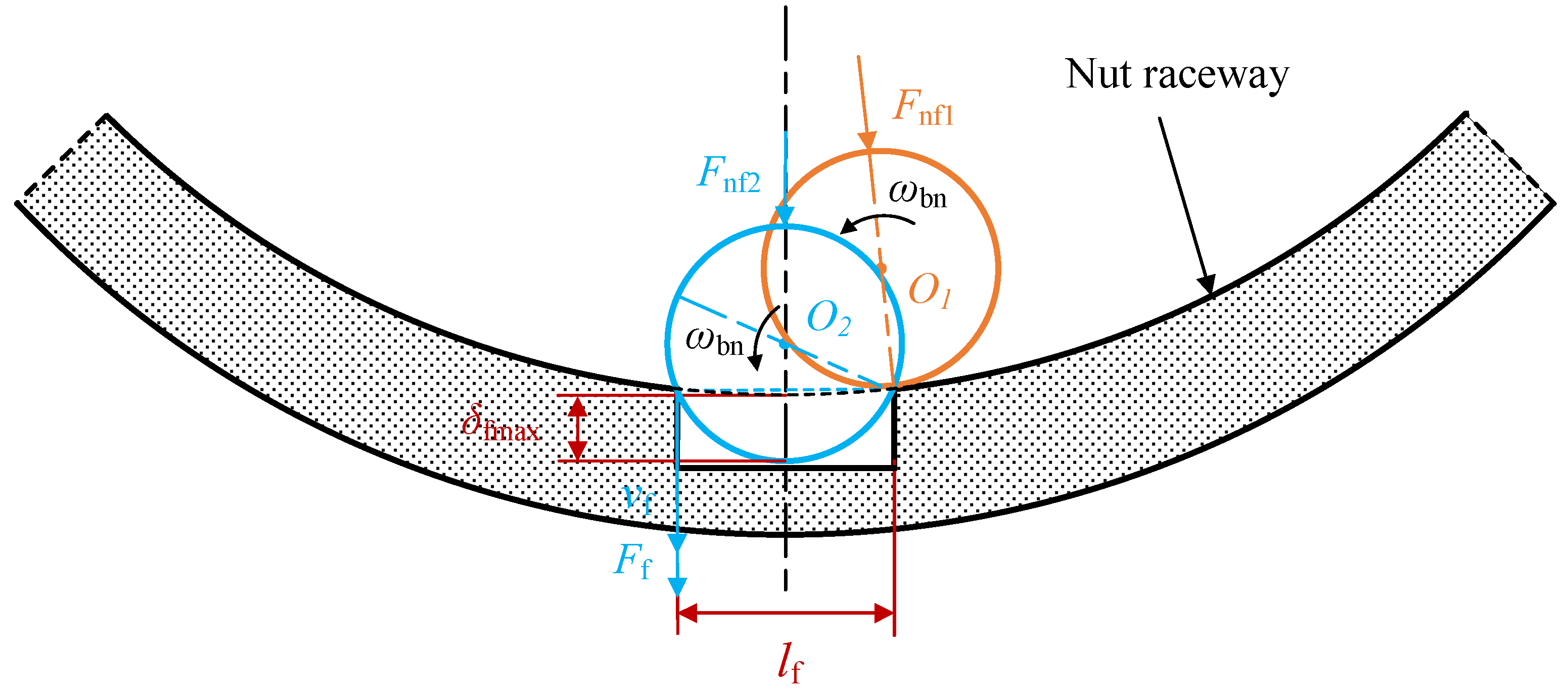
3. Dynamic Modeling under Faulty Conditions

Figure 7 shows the model when a ball passes through a spall in the nut raceway. Unlike the screw shaft and the balls, the nut raceway always bears a load during the EMA system operation. Therefore, a spalling fault is more likely to occur in the raceway of the nut, which is why the nut spalling fault is investigated in this paper. When the ball reaches the front edge of the fault, the support of the subsequent nut raceway disappears, but the pressure of the screw shaft on the ball still exists. Therefore, the ball rotates around the front edge and enters the spalling fault area under the pressure of the screw shaft.
As the ball gradually enters the spalling fault area, the elastic deformation of the ball gradually releases until the ball center reaches the fault centerline and the release amount reaches its maximum [31]. When passing through the fault centerline, the ball impacts the edge of the spall due to inertia, at which point the ball center crosses the fault centerline, the ball gradually leaves the spall and the elastic deformation of the ball gradually returns to the level under normal conditions [14].
The impact force of the ball on the fault edge (Ft) can be calculated by the theorem of momentum.
F f t f = m b v f cos β
where mb is the mass of the ball, and tf is the fault impact time. vf = ωbnlf is the linear velocity of the ball during the impact, where lf is the width of the fault crack, and ωbn is the angular velocity of the ball rotating around a point on the nut raceway. Ismail et al. provide the corresponding relationship between ωbn and the speed of ωbs [4].
ω bn = ω bs d s d b cos α d s + d b cos α
Although Equation (29) is based on the assumption that there is no slipping and no deformation, because the deformation of the ball is particularly small (about 10−7 m), as shown in Section 4, and the motion of each ball inside the nut is assumed to occur by pure rolling only, the results of Equation (29) are not strongly affected and can still be used for analysis of fault characteristics.
In addition to the impact force, the elastic restoring force of the ball when passing through the crack fault also changes to a certain extent. When a ball enters the spalling fault area, the vacancy on the subsequent nut raceway reduces the elastic deformation of the ball. Assuming that the release amount of elastic deformation of the ball when passing through the spall is δf, when the ball is entering the fault area, δf gradually increases until the ball center reaches the fault centerline and δf reaches its maximum value.
δ fmax = d b d b 2 l f 2 2
Then, as the ball center crosses the fault centerline, δf gradually decreases until the ball leaves the fault area and becomes 0 again. The calculation method of the total elastic restoring force of balls under faulty conditions is similar to that under normal conditions. The only difference is that δai and δni have to be changed into (δaiδf) and (δniδf), respectively, when calculating the elastic restoring force of the ball passing the fault. Then, the total elastic restoring force in the x, y and z directions under faulty conditions (Fnxf, Fnyf and Fnzf) can be obtained. After substituting Fnx, Fny and Fnz in Equation (17) with Fnxf, Fnyf and Fnzf, the equations of motion under faulty conditions can be expressed as follows:
M q ¨ + C q ˙ + K q = F f
where Ff is the vector of external forces under faulty conditions, which can be specifically expressed as follows:
F f = ( F sx 0 F nxf F nx 0 F nxf ( m n + m s ) g + F sy 0 F nyf m n g + F ny 0 F nyf F sz 0 F nzf F nz 0 F nzf T s 0 η F nz T m 0 + T m ( t ) )

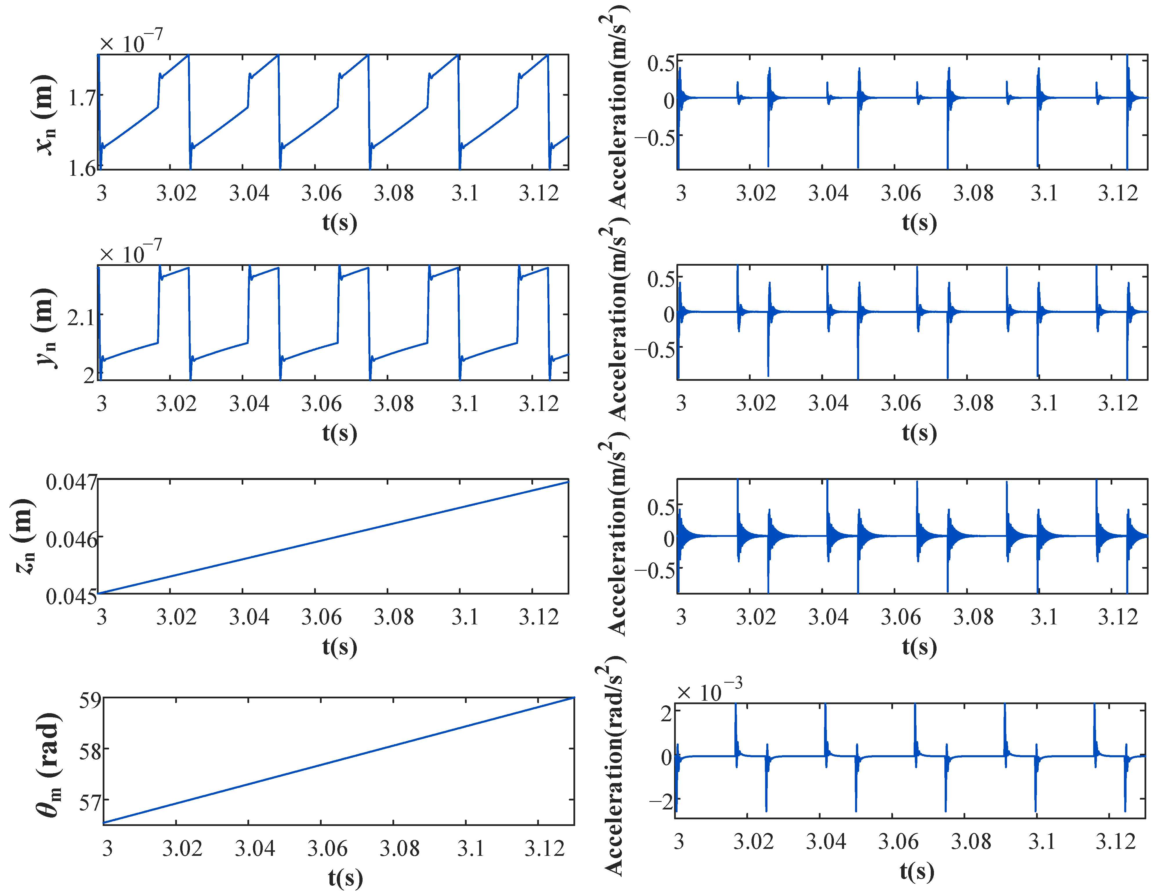
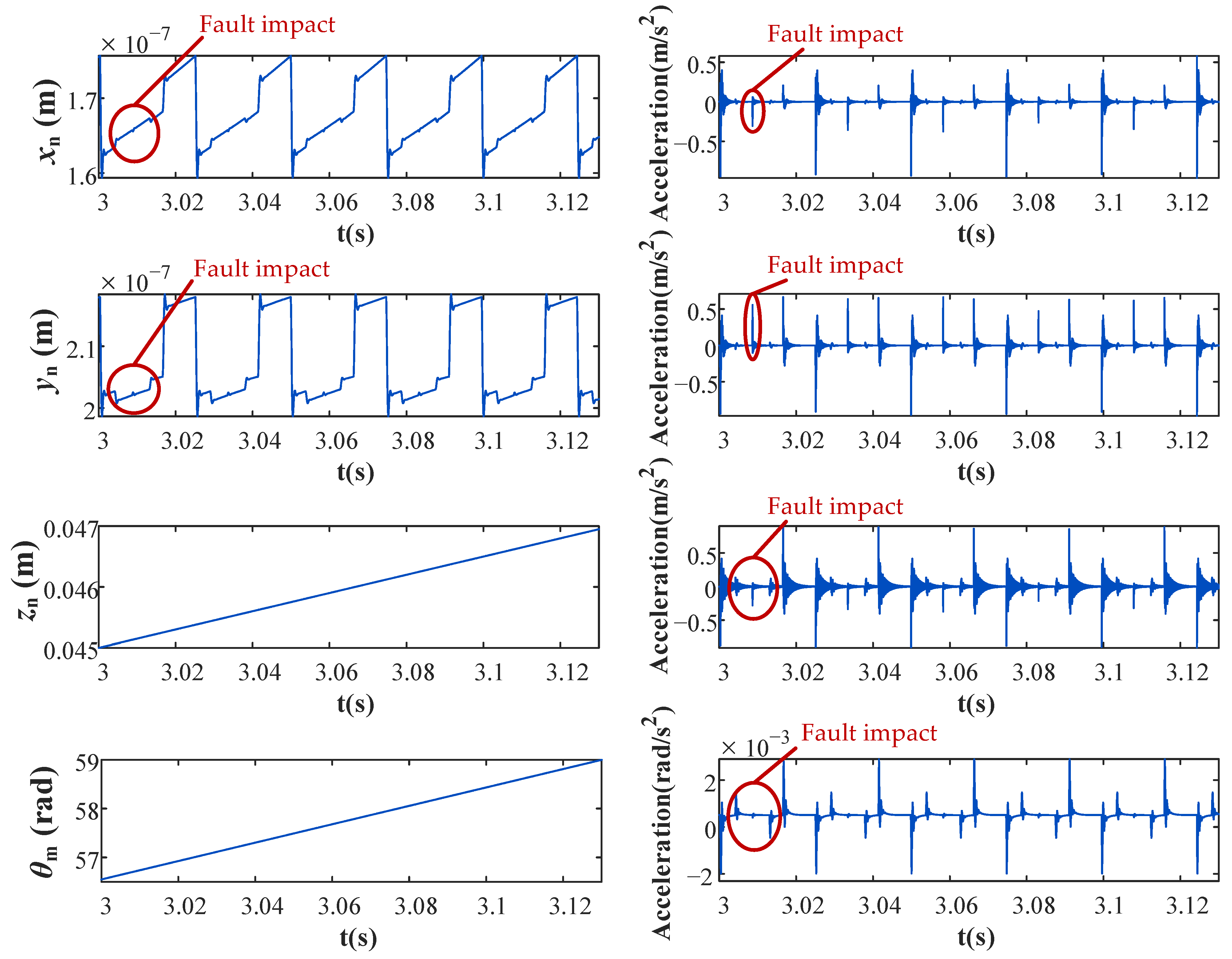
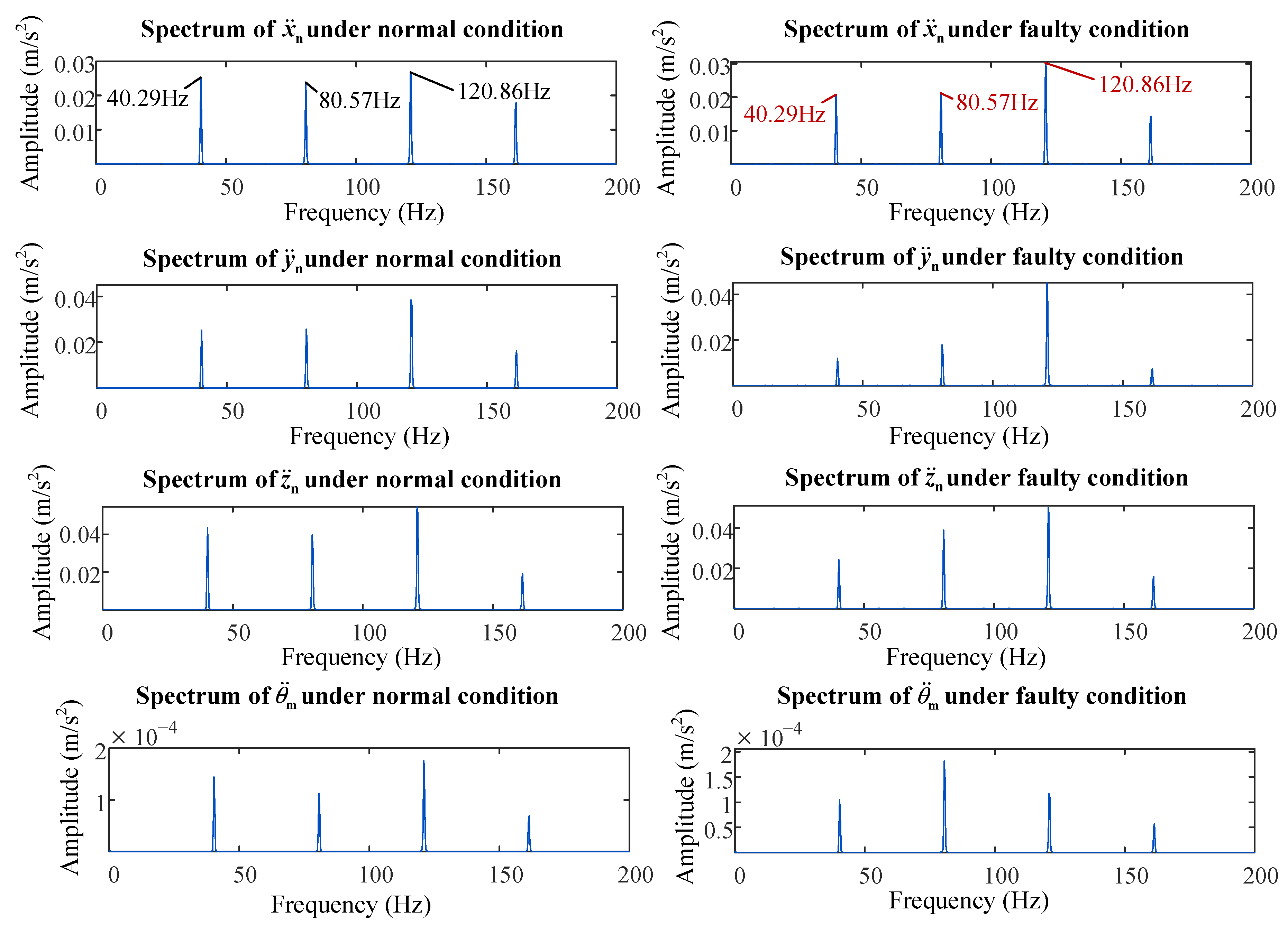
4. Simulation Results and Fault Characteristic Analysis

In order to facilitate experimental verification, we set the parameters of simulation based on the EMA test stand. The main parameters are listed in Table 1.
In this paper, the five-order Runge–Kutta method is used to solve the differential equations in Equations (17) and (31). Because the sampling frequency used in the experimental verification is 25.6 kHz, in order to make the simulation parameters consistent with the parameters adopted in actual experiments, the simulation step size is set to 3.90625 × 10⁻⁵ s. In the testing stage of the simulation, it is verified that such a step setting will not cause distortion of the simulation results. In order to ensure that the simulation signals contain enough screw shaft rotation cycles for subsequent analysis, the simulation time is set to 10 s. The geometric parameters, such as the ball diameter and the lead angle, are directly obtained from the manufacturer of the ball-screw pair. The damping coefficients can be calculated by the following equation [32]:
c = 2 ζ k m
where k is the stiffness of the component. In this paper, the calculated Hertz contact stiffnesses are adopted to calculate damping coefficients. m is the mass of the component, and ζ is the damping ratio, which is generally set between 0.02 and 0.1 based on engineering experience [33]. Therefore, in the simulation of the established model, ζ is set to 0.05, and according to the simulation results, such a parameter setting is appropriate.
The preload is set to 25 N. The reason for such a low preload is that the EMA test stand used for experimental verification was not designed to bear a large external load. Therefore, the EMA test stand only operates under a particularly small or even no external load, and the data acquired on this test stand are only used to verify the method proposed in this paper. Under such circumstances, a preload as low as 25 N is enough to ensure normal operation of the test stand. In the future studies, a test stand that is closer to actual EMA systems applied in engineering practice will be built and could support further research on the dynamic behaviors of actual EMAs used in aircraft. Then, experiments with parameters that are closer to those of EMAs in practical applications can be conducted and provide improved verification of the proposed model and identified fault characteristics.
Figure 8, Figure 9, Figure 10 and Figure 11 shows the simulation results when the angular velocity of the screw shaft is 6π rad/s (180 rpm), i.e., the rotation frequency is 3 Hz.
Figure 8 shows the displacement (angular displacement) response and acceleration (angular acceleration) response of the screw-shaft-related parameters (xs, ys, zs and θs) under normal conditions. Figure 9 shows the displacement (angular displacement) response and acceleration (angular acceleration) response of the nut-related parameters (xn, yn and zn), as well as the rotation of the motor output shaft (θm) in under normal conditions.
When the angular velocity of the screw shaft is constant, θs and θm increase linearly, and the rotation of the screw shaft drives the nut to move axially, so the axial displacement of the nut (zn) also increases, as shown in Figure 9. However, affected by the impacts of the balls entering and exiting the return device, the value of zn fluctuates slightly with increased rotation of the screw shaft. Because the amplitude of the fluctuation is far less than the value of zn (at about 10−7 level), it is difficult to directly determine the impacts of balls in the displacement response of zn, although they are much more obvious in the acceleration response.
As shown in Figure 8 and Figure 9, the impacts of the balls can be observed in the acceleration responses in the x, y and z directions. Whenever a ball exits (or enters) the raceway of the nut, the total elastic restoring force changes accordingly, and the nut displacement exhibits similar behavior to that of step responses, as shown in Figure 9. For the screw shaft, the impact generated by the balls entering and exiting the return device can be regarded as an external vibration excitation source, which generates impacts at different amplitudes but the same frequency. Then, the screw shaft exhibits forced vibration under the excitation of these impacts and the constraint of the bearings. Therefore, the displacement of the screw shaft exhibits behavior similar to that of impulse responses, as shown in Figure 8.
The displacement and acceleration responses of the system after the spalling fault is implanted into the model are shown in Figure 10 and Figure 11. Figure 10 shows that the responses of the screw-shaft-related parameters under faulty conditions are also impulse responses, similar to those under normal conditions. However, besides the two impacts of the ball entering and exiting the return device, there is another fault impact in both displacement and acceleration responses under faulty conditions. Furthermore, in the displacement and acceleration responses of the nut-related parameters, fault impacts can be more obviously identified. As shown in Figure 11, it is obvious that there is an additional fault impact between the two original impacts in the displacement responses of xn and yn.
Fast Fourier transform (FFT) is then applied to the acceleration responses to acquire the frequency spectra of the normal and fault models. Figure 12 shows the acceleration spectra of the screw-shaft-related parameters under normal and fault conditions. The ball passage frequency (fb), which is at about 40.29 Hz, can be observed in the normal frequency spectra. The harmonics of the ball passage frequency can also be found in the spectra. In the fault spectrum, the positions of fb and each of its harmonics are roughly the same as those in the normal spectra, despite the change in amplitude. After the spalling fault occurs, the amplitude at the first and second harmonics of fb decrease, whereas the amplitude at the third harmonic increases. This phenomenon can also be observed in the frequency spectra of nut-related parameters, as shown in Figure 13. This is because when the spalling fault occurs, the number of impacts in the same ball passage cycle changes from two to three, resulting in an increase in the amplitude at the third harmonic of fb in the frequency spectra obtained by FFT and a decrease at the first and second harmonics of fb.
Assuming that Pn1, Pn2 and Pn3 are the peak values of the first three harmonics of fb in the normal spectra, Pf1, Pf2 and Pf3 are the peak values of the first three harmonics of fb in the faulty spectra. The specific values of Pn1, Pn2, Pn3, Pf1, Pf2 and Pf3 can be obtained through the peak-detection algorithms. Based on the amplitude-increasing phenomenon described in the previous paragraph, we propose a numerical calculation method for the characteristics of nut spalling faults to describe the decrease and increase in the amplitudes of the harmonics of fb after the spalling fault occurs.
F C = P n 1 P f 1 P n 1 + P n 2 P f 2 P n 2 + P f 3 P n 3 P n 3
The proposed FC values of the frequency spectra of all eight parameters (xs, ys, zs, θs, xn, yn, zn and θm) are calculated; the results are shown in Figure 14. The FC values in the y direction of the nut and the screw shaft are the highest among all eight parameters, with values of 1.4072 and 0.9949, respectively. The FC values in the x and z directions are smaller than those in the y direction, which indicates that the spalling fault has less of an influence on the vibration in the x and z directions. However, the FC values in the torsional direction are less than 0, and the FC value of θm reaches −0.6752, in contrast to the fault characteristic described in this paper. This may because that the acceleration amplitudes of θm caused by the vibration of the screw shaft and the nut are particularly small under both normal and faulty conditions, which makes the influence of the fault on θm appear to be abnormal. Therefore, the FC values in the torsional direction cannot be used as the features of the nut spalling fault.
In summary, the FC values in the y direction are the most suitable to be used as a fault feature. However, this is only the result obtained under a certain rotational frequency of the screw shaft. Further exploration is necessary to obtain fault characteristics suitable for different working conditions.

5. Experimental Verification

In order to further verify the accuracy and effectiveness of the models established in this paper, we use an EMA test stand built in a laboratory environment to verify the proposed dynamic models. The main components of the test stand are shown in Figure 15. The motor used in the test stand is a Siemens 1FL6042 motor, and the ball-screw pair is a TBI sfv2505 ball-screw pair. The six accelerometers used in the test stand are Yangzhou ymc-162A10T single-axial low-impedance voltage-output micro accelerometers with a range of ±500 g (g refers to the gravitational acceleration) and a sensitivity of 10 mV/g. The accelerometers are installed to measure the acceleration signals of the screw shaft and the nut in the x, y and z directions. Because it is difficult to directly measure the vibration in the torsional direction, the angular parameters in the simulation model are not verified in this paper. In addition to acquiring the vibration signals of the ball-screw pair, a photoelectric sensor is adopted in the test stand to monitor the angular velocity of the screw shaft. The acquisition equipment used in the data acquisition system comprises three NI9234 sound and vibration input modules and an NI cDAQ-9174 chassis. The sampling frequency is set to be 25.6 kHz, and the duration of measurement is 5 s.
Owing to the rotation of the screw shaft during test stand operation, it is difficult to directly obtain the vibration signal of the screw shaft. Moreover, owing to the raceway groove with a lead angle, the contour of the screw shaft changes continuously during the rotation, so it is also difficult to directly acquire the displacement signal of the screw shaft. Therefore, as an alternative, the accelerometers are installed on the base of the supporting bearings to obtain the vibration signals of the screw shaft. In order to eliminate the interference caused by motor vibration, the positions of the screw accelerometers are set on the bearing base far away from the motor output shaft, namely the base of bearing #2.
The faulty nut used in the test stand is machined from a normal sfv2505 nut. A 1 mm gap is cut in the y direction of the nut by the wire cutting method to simulate the spall generated during EMA operation. The faulty nut is shown in Figure 16.
After obtaining the acceleration signals acquired by all six accelerometers, it is necessary to denoise the original signals and highlight the fault characteristics. In this paper, we adopt the wavelet domain denoising as the denoising method, with the aim of reducing the high-frequency components in the acceleration signals and focusing on the frequency components around fb and its harmonics. After wavelet domain denoising, the FFT is used to obtain the frequency spectrum of each acceleration signal, as shown in Figure 17 and Figure 18.

6. Discussion

Figure 17 shows the experimental acceleration spectra of the screw-shaft-related parameters (xs, ys and zs) under normal and faulty conditions. It is difficult to determine the ball-passing frequency (40.29 Hz) in the frequency spectrum in the x direction of the screw shaft. Although there are similar frequency spikes, their amplitudes are far smaller than that of the main frequency component and are almost covered up by other components. This may be caused by the lack of external load in the x direction. The screw shaft needs to drive the nut assembly in the z direction and bear the gravity of the nut assembly in the y direction. However, the screw shaft hardly bears any load in the x direction. As a result, the vibration amplitude of the screw shaft excited by the impact of the balls in the x direction is relatively small and is easily covered up by other noises. In contrast, in the normal acceleration spectra of the y and z directions, amplitude peaks can be found at 42.9 Hz, as well as near the second (85.9 Hz) and third (128.8 Hz) harmonics. Although frequency peaks at three harmonics can be observed in the experimental frequency spectra, there is still a difference between the experimental ball-passage frequency (42.9 Hz) and the simulated frequency (40.29 Hz), possibly because the output speed of the motor is not stable during EMA test stand operation.
In addition, in the faulty acceleration spectra in the y and z directions, obvious frequency spikes can be found at these three frequencies. Compared with normal conditions, the amplitudes at the first and second harmonics decrease, whereas the that at the third harmonic increases, which is also consistent with the phenomenon reported in the analysis of simulation results in this paper.
However, as shown in Figure 17, the frequency spectra of screw-shaft-related parameters also contain many frequency components that are not related to the fb, especially around 100.2 Hz and 114.5 Hz. In some spectra, the amplitudes of these two frequencies even exceed the amplitudes of fb and its harmonics. Owing to these interference components, it is difficult to directly use the same peak-detection algorithm as that used in the simulation analysis to extract fault features from the acquired signal of each screw-shaft-related parameter. Therefore, the proposed method should be supplemented by more advanced signal processing methods.
Figure 18 shows the acceleration spectra of the nut-related parameters (xn, yn and zn) under normal and faulty conditions. Similar to the screw shaft acceleration spectrum, it is difficult to determine the frequency components similar to the ball passage frequency (40.29 Hz) in the spectra of xn, which are basically covered by the interference components of approximately 100.1 Hz and 114 Hz. Although the corresponding amplitude peaks at approximately 42.9 Hz and its harmonics can be found in the frequency spectra of zn, there are also many components that are independent of the ball-passage frequency, causing serious interference.
However, in the frequency spectra of yn, especially in the faulty spectrum, three amplitude peaks occur at 42.9 Hz, 85.8 Hz and 130 Hz, and the peaks at 42.9 Hz and 130 Hz considerably exceed other interference components. A comparison of the faulty spectrum with the normal spectrum shows that the amplitude at the third harmonic increases obviously, whereas those at the first and second harmonics decrease. Therefore, the signals of yn are the most suitable for extraction of fault features among all six parameters.
Then, the corresponding amplitude values are determined around fb (42.9 Hz), 2fb (85.9 Hz) and 3fb (128.8 Hz or 130 Hz) in the frequency spectra of ys, zs, yn and zn, as shown in Table 2.
When the obtained amplitude values are input into Equation (34), the fault characteristic FC values of the four parameters can be obtained, as shown in Figure 19. The FC values in the y direction are higher than those in the z direction, which indicates that the nut spalling fault has a stronger influence on the y direction than the z direction. This verifies the amplitude-increasing phenomenon observed in the simulation analysis to a certain extent. However, there are still some differences between the experimental values of FC and the simulated values of FC, especially the FC values of ys. This is because the vibration of the screw shaft is not directly acquired by the accelerometers, and the influence of the nut spalling fault is reduced by the supporting bearings. Therefore, in order to ensure more accurate and stable fault features for the subsequent fault diagnosis or prognosis work, further exploration is necessary with respect to a numerical calculation method for nut spalling fault characteristics.

7. Conclusions

With the help of the Lagrangian energy method, an eight-DOF dynamic model containing typical mechanical components of an EMAs is established in this paper. By obtaining the impact force and the relationship between the total elastic restoring forces and the change in ball deformation when a spall occurs in the raceway of the nut, a faulty dynamic model of an EMA mechanical transmission is established. In the analysis of the simulation results of the established models, the dynamic behaviors of the ball-screw pair in the EMA system are described in detail, and the coupling effect of the displacements and accelerations in the axial and torsional direction is reflected. After further exploration under different working conditions, the established dynamic models of an EMA mechanical transmission can serve as a reference for establishing physical models of EMA systems or generating available data for the data-driven fault diagnosis of EMA systems.
According to a comparison of the amplitudes of the simulated accelerations of the normal and faulty models, the acceleration amplitude at the third harmonic of the ball passage frequency increases, whereas the amplitudes at the first and second harmonics decrease in the faulty model. A fault indicator of nut spalling is proposed based on this phenomenon. Then, the FC values of all eight parameters are calculated, and it is concluded that the parameters in the radial direction have the highest FC values and are suitable for extracting fault features. Although restricted by numerous assumptions adopted for dynamic modeling, the analysis of the simulation results in this paper can still provide a new feature extraction method for EMA fault diagnosis and inform the installation of the accelerometers in EMA systems.
The effectiveness of the established eight-DOF dynamic models and the identified phenomenon is verified by experiments conducted on an EMA test stand in a laboratory environment. However, there is still considerable noise interference in the acquired signals, as well as certain errors between the simulation and experiment results of the ball passage frequency and FC values. Therefore, in subsequent research, the influence of the motor will be considered to further improve the accuracy of the established model and the proposed FC calculation method. Furthermore, additional signal processing methods are needed to realize engineering applications in actual EMA systems. Moreover, a test stand using actual aircraft EMAs will be built to ensure experimental results that are closer to practical aviation applications.

Author Contributions

Conceptualization, Z.Y., Y.Y., G.S., L.C. and N.H.; methodology, Z.Y., Y.Y., G.S. and N.H.; software, Z.Y.; validation, Z.Y. and Y.Y.; formal analysis, Z.Y. and Y.Y.; investigation, Z.Y.; resources, N.H. and G.S.; data curation, Z.Y.; writing—original draft preparation, Z.Y.; writing—review and editing, Y.Y., G.S., L.C. and N.H.; visualization, Z.Y. and L.C.; supervision, N.H. and G.S.; project administration, N.H.; funding acquisition, N.H. and G.S. All authors have read and agreed to the published version of the manuscript.

Funding

This research is supported by the National Natural Science Foundation of China, grant number 51975576.

Institutional Review Board Statement

Not applicable.

Informed Consent Statement

Not applicable.

Data Availability Statement

No new data were created or analyzed in this study. Data sharing is not applicable to this article.

Conflicts of Interest

The authors declare no conflict of interest.

References

  1. Mazzoleni, M.; Di Rito, G.; Previdi, F. Electro-Mechanical Actuators for the More Electric Aircraft, 1st ed.; Springer: Cham, Switzerland, 2021; Volume 2021. [Google Scholar]
  2. Yin, Z.; Hu, N.; Chen, J.; Yang, Y.; Shen, G. A review of fault diagnosis, prognosis and health management for aircraft electromechanical actuators. IET Electr. Power Appl. 2022; early view. [Google Scholar]
  3. Balaban, E.; Bansal, P.; Stoelting, P.; Saxena, A.; Goebel, K.F.; Curran, S. A diagnostic approach for electro-mechanical actuators in aerospace systems. In Proceedings of the 2009 IEEE Aerospace Conference, Big Sky, MT, USA, 7–14 March 2009; pp. 1–13. [Google Scholar]
  4. Ismail, M.A.A.; Balaban, E.; Spangenberg, H. Fault detection and classification for flight control electromechanical actuators. In Proceedings of the 2016 IEEE Aerospace Conference, Big Sky, MT, USA, 5–12 March 2016; pp. 1–10. [Google Scholar]
  5. Balaban, E.; Saxena, A.; Narasimhan, S.; Roychoudhury, I.; Goebel, K. Experimental validation of a prognostic health management system for electro-mechanical actuators. In Infotech@aerospace; American Institute of Aeronautics and Astronautics: St. Louis, MO, USA, 2011. [Google Scholar]
  6. Balaban, E.; Saxena, A.; Narasimhan, S.; Roychoudhury, I.; Goebel, K.; Koopmans, M. Airborne Electro-Mechanical Actuator Test Stand for Development of Prognostic Health Management Systems. In Proceedings of the Annual Conference of the Prognostics and Health Management Society, Portland, OR, USA, 10–16 October 2010. [Google Scholar]
  7. Balaban, E.; Saxena, A.; Goebel, K.; Byington, C.; Watson, M.; Bharadwaj, S.; Smith, M.; Amin, S. Experimental data collection and modeling for nominal and fault conditions on electro-mechanical actuators. In Proceedings of the Annual Conference of the Prognostics and Health Management Society, San Diego, CA, USA, 27 September–1 October 2009; pp. 1–15. [Google Scholar]
  8. Bodden, D.S.; Clements, N.S.; Schley, B.; Jenney, G. Seeded failure testing and analysis of an electro-mechanical actuator. In Proceedings of the 2007 IEEE Aerospace Conference, Big Sky, MT, USA, 3–10 March 2007; pp. 1–8. [Google Scholar]
  9. Wang, C.; Tao, L.; Ding, Y.; Lu, C.; Ma, J. An adversarial model for electromechanical actuator fault diagnosis under nonideal data conditions. Neural Comput. Appl. 2022, 34, 5883–5904. [Google Scholar] [CrossRef]
  10. Hussain, Y.M.; Burrow, S.; Henson, L.; Keogh, P. A high fidelity model based approach to identify dynamic friction in electromechanical actuator ballscrews using motor current. Int. J. Progn. Health Manag. 2020, 9. [Google Scholar] [CrossRef]
  11. Mazzoleni, M.; Maccarana, Y.; Previdi, F. A comparison of data-driven fault detection methods with application to aerospace electro-mechanical actuators. IFAC-PapersOnLine 2017, 50, 12797–12802. [Google Scholar] [CrossRef]
  12. Chirico, A.J.; Kolodziej, J.R. A data-driven methodology for fault detection in electromechanical actuators. J. Dyn. Syst. Meas. Control 2014, 136, 041025. [Google Scholar] [CrossRef]
  13. Yang, T.; Cao, X.; Yang, J. Fault detection and isolation of the electro-mechanical actuator based on bit. IOP Conf. Ser. Mater. Sci. Eng. 2020, 790, 012163. [Google Scholar] [CrossRef]
  14. Ismail, M.A.A.; Balaban, E.; Windelberg, J. Spall fault quantification method for flight control electromechanical actuator. Actuators 2022, 11, 29. [Google Scholar] [CrossRef]
  15. Hospital, F.; Budinger, M.; Reysset, A.; Maré, J.-C. Preliminary design of aerospace linear actuator housings. Aircr. Eng. Aerosp. Technol. 2015, 87, 224–237. [Google Scholar] [CrossRef]
  16. Liu, C.; Zhao, C.; Wen, B. Dynamics analysis on the mdof model of ball screw feed system considering the assembly error of guide rails. Mech. Syst. Signal Process. 2022, 178, 109290. [Google Scholar] [CrossRef]
  17. Xu, M.; Cai, B.; Li, C.; Zhang, H.; Liu, Z.; He, D.; Zhang, Y. Dynamic characteristics and reliability analysis of ball screw feed system on a lathe. Mech. Mach. Theory 2020, 150, 103890. [Google Scholar] [CrossRef]
  18. Liu, J.; Ou, Y. Dynamic axial contact stiffness analysis of position preloaded ball screw mechanism. Adv. Mech. Eng. 2019, 11, 1687814018819289. [Google Scholar] [CrossRef]
  19. Gu, J.; Zhang, Y. Dynamic analysis of a ball screw feed system with time-varying and piecewise-nonlinear stiffness. Proc. Inst. Mech. Eng. Part C J. Mech. Eng. Sci. 2019, 233, 6503–6518. [Google Scholar] [CrossRef]
  20. Guo, C.; Chen, L.; Ding, J. A novel dynamics model of ball-screw feed drives based on theoretical derivations and deep learning. Mech. Mach. Theory 2019, 141, 196–212. [Google Scholar] [CrossRef]
  21. Bertolino, A.C.; Sorli, M.; Jacazio, G.; Mauro, S. Lumped parameters modelling of the emas’ ball screw drive with special consideration to ball/grooves interactions to support model-based health monitoring. Mech. Mach. Theory 2019, 137, 188–210. [Google Scholar] [CrossRef]
  22. Bertolino, A.C.; Mauro, S.; Jacazio, G.; Sorli, M. Multibody dynamic model of a double nut preloaded ball screw mechanism with lubrication. In Proceedings of the ASME 2020 International Mechanical Engineering Congress and Exposition, Virtual Online, 16–19 November 2020. [Google Scholar]
  23. Vicente, D.; Hecker, R.; Villegas, F.; Flores, G. Modeling and vibration mode analysis of a ball screw drive. Int. J. Adv. Manuf. Technol. 2012, 58, 257–265. [Google Scholar] [CrossRef]
  24. Feng, G.-H.; Pan, Y.-L. Investigation of ball screw preload variation based on dynamic modeling of a preload adjustable feed-drive system and spectrum analysis of ball-nuts sensed vibration signals. Int. J. Mach. Tools Manuf. 2012, 52, 85–96. [Google Scholar] [CrossRef]
  25. Hu, N.; Hu, L.; Cheng, Z. Mechanical Vibration; National University of Defense Technology Press: Changsha, China, 2017; p. 335. [Google Scholar]
  26. Chen, J.S.; Huang, Y.K.; Cheng, C.C. Mechanical model and contouring analysis of high-speed ball-screw drive systems with compliance effect. Int. J. Adv. Manuf. Technol. 2004, 24, 241–250. [Google Scholar] [CrossRef]
  27. Vashisht, R.K.; Peng, Q. Online chatter detection for milling operations using lstm neural networks assisted by motor current signals of ball screw drives. J. Manuf. Sci. Eng. 2021, 143, 011008. [Google Scholar] [CrossRef]
  28. Xu, M.; Zhang, H.; Liu, Z.; Li, C.; Zhang, Y.; Mu, Y.; Hou, C. A time-dependent dynamic model for ball passage vibration analysis of recirculation ball screw mechanism. Mech. Syst. Signal Process. 2021, 157, 107632. [Google Scholar] [CrossRef]
  29. Varanis, M.V.M.; Mereles, A.G.; Silva, A.L.; Balthazar, J.M.; Tusset, A.M.; Oliveira, C. Modeling and experimental validation of two adjacent portal frame structures subjected to vibro-impact. Lat. Am. J. Solids Struct. 2019, 16, e179. [Google Scholar] [CrossRef] [Green Version]
  30. Liu, Z.; Xu, M.; Zhang, H.; Miao, H.; Li, Z.; Li, C.; Zhang, Y. Nonlinear dynamic analysis of ball screw feed system considering assembly error under harmonic excitation. Mech. Syst. Signal Process. 2021, 157, 107717. [Google Scholar] [CrossRef]
  31. Zhang, Y. Research on Contact Mechanics Vibration Model and Feature Extraction Method of Ball Screw. Master’s Thesis, Southeast University, Nanjing, China, 2013. [Google Scholar]
  32. Inman, D.J. Single-degree-of-freedom systems. In Vibration with Control; John Wiley & Sons, Ltd.: Hoboken, NJ, USA, 2006; pp. 1–38. [Google Scholar]
  33. Ni, Z. Vibration Mechanics; Xi’an Jiaotong University Press: Xi’an, China, 1989; p. 521. [Google Scholar]
Figure 1. Basic structures of EMA systems [15]. (a) EMA using the screw shaft as the driving component; (b) EMA using the nut as the driving component.
Actuators 11 00226 g001
Figure 2. Simplified model of the EMA test stand.
Actuators 11 00226 g002
Figure 3. Dynamic model of an EMA mechanical transmission. (a) Axial model; (b) radial model.
Actuators 11 00226 g003
Figure 4. Deformation of a single ball when only preload is applied.
Actuators 11 00226 g004
Figure 5. Change in nut displacements after the ith ball bears the load.
Actuators 11 00226 g005
Figure 6. Fni direction of each ball in the ball nut.
Actuators 11 00226 g006
Figure 7. Model of a ball passing through a rectangular spall in the nut raceway.
Actuators 11 00226 g007
Figure 8. Displacement responses and acceleration responses of the screw-shaft-related parameters under normal conditions.
Actuators 11 00226 g008
Figure 9. Displacement responses and acceleration responses of the nut or motor output shaft-related parameters under normal conditions.
Actuators 11 00226 g009
Figure 10. Displacement responses and acceleration responses of the screw-shaft-related parameters under faulty conditions.
Actuators 11 00226 g010
Figure 11. Displacement responses and acceleration responses of the nut or motor output shaft-related parameters under faulty conditions.
Actuators 11 00226 g011
Figure 12. Frequency spectra of the screw shaft related parameters under normal and faulty conditions.
Actuators 11 00226 g012
Figure 13. Frequency spectra of the nut or motor output shaft-related parameters under normal and faulty conditions.
Actuators 11 00226 g013
Figure 14. Simulated FC values of all eight parameters.
Actuators 11 00226 g014
Figure 15. Main components of the EMA test stand.
Actuators 11 00226 g015
Figure 16. Faulty nut used in the EMA test stand.
Actuators 11 00226 g016
Figure 17. Experimental acceleration spectra of the screw-shaft-related parameters under normal and faulty conditions (the acceleration values are calculated from the voltage values, which are directly measured by the accelerometers).
Actuators 11 00226 g017
Figure 18. Experimental acceleration spectra of the nut-related parameters under normal and faulty conditions (the acceleration values are calculated from the voltage values, which are directly measured by the accelerometers).
Actuators 11 00226 g018
Figure 19. Experimental FC values of four parameters.
Actuators 11 00226 g019
Table 1. Main parameters of the normal/faulty simulation model.
ParameterValue
Ball diameter, db (m)0.003175
Diameter of the screw shaft pitch circle, ds (m)0.025
Lead angle, β (rad)0.063576
Contact angle, α (rad)0.25π
Number of turns of the nut raceway, Ns4.8
Mass of the nut, mn (kg)0.6605
Mass of the screw shaft, ms (kg)3.4285
Axial preload, Fp (N)25
Width of nut spalling fault, lf (m)0.001
Screw shaft rotating speed (rpm) 180
Table 2. Amplitude values around fb, 2fb and 3fb.
SpectrumAmplitude Increase Rate (%)
fb2fb3fb
ys46.9832−11.2515111.486
zs59.3389−15.192988.1544
yn10.7598−58.407658.8222
zn22.3039−40.756471.6203
Publisher’s Note: MDPI stays neutral with regard to jurisdictional claims in published maps and institutional affiliations.

