Numerical Study of the Fish-like Robot Swimming in Fluid with High Reynolds Number: Immersed Boundary Method

Abstract

Fish-like robots have been widely used in intelligent surveillance and investigation because of their high swimming efficiency and low traveling noise. Numerical simulations are usually selected to simulate the movement modes and hydrodynamic characteristics of fish-like robots during design and manufacture. However, the body-fitted grid method traditionally utilized in numerical simulations often has difficulty dealing with moving solid boundaries. In this work, the immersed boundary method, superior in handling the moving boundary conditions, is employed to simulate the movement of a fish-like robot swimming in high Reynolds number flows in combination with the RANS turbulence model. The numerical method is first validated using a fluid flowing over a square block, and the corresponding results are in good agreement with the ones reported in reference. Then, the swing of the fish-like robot under three different Reynolds numbers is studied. The lift coefficient and the drag coefficient of the fish-like robot decrease with increasing the Reynolds number. This paper provides remarkable support for future designs and applications of fish-like robots.

1. Introduction

Aracri et al. [1] introduced the idea that due to climate change, marine pollution, and the development of offshore energy, further exploration of the ocean is facing increasing pressure. Underwater fish-like robots have incomparable advantages such as high efficiency, high maneuverability, and strong camouflage, unlike ordinary artificial underwater vehicles. Thus, underwater fish-like robots have a very important impact on deep-sea exploration and industrial applications. Marcin et al. [2] investigated the speed, motion noise, and suffered force of an underwater autonomous fish-like robot. The noise levels of two fish-like robots with different driving modes were intensively measured and analyzed. Glaze et al. [3] numerically studied different shapes and arrangements of the caudal fin of a fish-like robot, and found that a subcarangiform’s wing shape gave rise to the best performance. Chen et al. [4] designed a tuna-like robot with a three-dimensional spiral tracking system for detecting deep-sea cages, and proposed a path definition method of the polar coordinate that simplified the definition of the reference path in the cage detection process. Utter et al. [5] set up an experimental platform for fabricating, operating, and verifying fish-like robots. In addition to research on a single fish-like robot, the behaviors of a group of fish-like robots were also studied. Shao et al. [6] experimentally verified the feasibility and effectiveness of a bionic fish robot by implementing collaborative transportation tasks. These traditional experimental studies of fish-like robots are extremely time-consuming and expensive. Therefore, the high-efficiency numerical method has been increasingly applied to investigate the movement and the interactions with the surrounding fluid of fish-like robots. A submerged body that turned its volume periodically was studied as a model system for sustained drag cancellations [7]. The corresponding results identified the role of added-mass recovery in the context of aquatic propulsion and resonance. The influence of the variations in body shape on the continuous swimming speed and the efficiency was also studied by using large-scale structural deformations [8]. It was found that the average swimming speed at natural frequency was four times the length of the structure per second, and the quasi-propulsion efficiency was 90%. The excitation of natural frequency led to a rapid decline in efficiency and swimming speed.

Armanini et al. [9] designed and developed an underwater robot inspired by flagella. Propellers, driven by simple knobs and energy stored by soft materials when interacting with surrounding fluids, had different spiral shapes to generate propulsion. Liu et al. [10,11,12] simulated the movement of tadpoles and the two- and three-dimensional flows around the wings of insects by utilizing the dynamic grid-based Navier–Stokes (N-S) equation solver. Carling et al. [13] used a dynamic structural mesh coupled with a differential solver to study the autonomous swimming of fish under two-dimensional conditions. Togashi et al. [14] used a numerical method with an overlapping nonstructural grid to simulate the trajectory of bee wings under three-dimensional conditions; Zhang et al. [15] proposed a hybrid dynamic mesh-generation technology of two-dimensional deformers to simulate the flow field surrounding fishes. Maertens et al. [16] introduced the concept of quasiefficiency and used kinematic simulation studies of carangiform and anguilliform shapes to demonstrate that low efficiency may be caused by fuselage thrusters or hydrodynamic interactions rather than by frictional resistance because the pressure was the major contributor to thrust and drag when the Reynolds number was 5000.

Most of the traditional numerical simulation methods use the body-fitted grid method, the disadvantage of which is that they cannot deal with the dynamic boundary problem well. Therefore, an immersed boundary method, with a feature of independence between the fixed-wall boundary grid and the background grid, was proposed by Peskin [17] in 1972. This method was initially used to solve the elastic boundary problem, which is similar to the determination of visceral valve flow. It is realized by the following steps: The force at the boundary is obtained by Hooker’s law, combined with the shape variation of the boundary, and then interpolated to the background grid through the regularization function to obtain the force in the flow field. The source term of the obtained force is then added to the N-S equation to simulate the force induced by the interactions between the fluid and the solid. The force is thus generated by interaction. The background grid used by the immersion boundary method is the Cartesian grid. Weymouth and Yue [18] developed a new advective and reconstructed fluid volume (VOF) algorithm, which is suitable for 2D and 3D flows. A computationally efficient and second-order VOF reconstruction method was presented, which used no inversions to determine the normal direction of the interface. This method provided a new idea for solving Cartesian meshes. However, the traditional immersed boundary method cannot be applied to deal with the flow of high Reynolds numbers. In this work, we employ the multidirect forcing and immersed boundary methods with the high-order finite difference method and RANS turbulence model to enable the simulation of the high Reynolds number flow caused by swinging fish-like robots.

The paper is organized in the following manner: In Section 2, we present the mathematical model and the numerical method. In Section 3, various numerical experiments are performed to investigate the effect of a high Reynolds number on a fish-like robot swimming in water. Conclusions are drawn in Section 4.

2. Numerical Method

2.1. Governing Equation

The dimensionless governing equations of the incompressible flow in the whole calculation domain Ω are

$$\nabla \cdot u=0,$$

(1)

$$\frac{\partial u}{\partial t}+u\cdot \nabla u=-\nabla P+\frac{1}{Re}{\nabla }^{2}u+f$$

(2)

where $u$ and $P$ are the velocity field and the pressure, respectively; $Re$ is the Reynolds number defined as $Re=\rho ul/\mu$, with $\rho$, $l$, and $\mu$ representing the fluid density, characteristic length of the flow field, and viscosity of the fluid, respectively; $f$ is the external force imposed on the flow field, which is the interaction force between the fluid and the immersed boundary, and is expressed as

$$f\left(x\right)={\int }_{\Omega }{F}_k(x_k)·\delta \left(x-x_k\right)d{x}_k,$$

(3)

where $\delta \left(x-x_k\right)$ is the Dirac delta function, $x_k$ is the position of Lagrange point set on the immersed boundary, $x$ is the position of Euler grid, and $F_k\left(x_k\right)$ is the force applied to Lagrange point.

In this paper, a three-step time splitting scheme is adopted to derive the flow field. Firstly, the velocity is increased from the $n$ time level to the first intermediate layer * by solving the diffusion equation, which is expressed as [19]

$$S^n=\frac{u^{*}-u^n}{\Delta t}$$

(4)

where $S$ is the convection and the diffusion terms of the momentum equation. In this paper, the second-order ADAM-Bashford method is used for time discretization. Then, S can be rewritten as

$$S^n=\frac{3}{2}{(-\nabla \cdot \left(uu\right)+\frac{1}{Re}{\nabla }^{2}u)}^n-\frac{1}{2}{(-\nabla \cdot \left(uu\right)+\frac{1}{Re}{\nabla }^{2}u)}^{n-1}$$

(5)

The convection and diffusion terms of the momentum equation are discretized by the second-order upwind scheme and the central difference scheme, respectively. The discretization scheme is given as

$$\frac{u\partial u}{\partial x}=\frac{1}{2\Delta x}(u^{+}\left(3u_{i,j}-4u_{i-1,j}+u_{i-2,j}+u^{-}\left(-u_{i+2,j}+4u_{i+1,j}-3u_{i,j}\right)\right)$$

(6)

where

$$u^{+}=0.5\left(u_{i,j}+\left|u_{i,j}\right|\right),$$

(7)

$$u^{-}=0.5\left(u_{i,j}-\left|u_{i,j}\right|\right)$$

(8)

Secondly, this work proceeds at the first intermediate speed including the pressure term

$$\frac{u^{**}-u^{*}}{\mathsf{\Delta }t}=-\nabla p^{n+1}$$

(9)

Applying divergence to both sides, Equation (9) becomes

$$\frac{\nabla \cdot u^{**}-\nabla \cdot u^{*}}{\mathsf{\Delta }t}=-{\nabla }^2{p}^{n+1}$$

(10)

Due to the mass conservation

$$\nabla \cdot u^{**}=0$$

(11)

Substituting Equation (11) into Equation (10), we obtain

$${\nabla }^2{p}^{n+1}=\frac{1}{\mathsf{\Delta }t}\nabla \cdot u^{*}$$

(12)

The pressure gradient can be achieved by solving the equation above, with which we can thus derive the second intermediate velocity in Equation (11).

Finally, the velocity $u^{n+1}$ of the time layer of $n+1$ can be obtained by calculating the boundary force under the Euler grid, which is given as

$$\frac{u^{n+1}-u^{**}}{\mathsf{\Delta }t}=f^{n+1}$$

(13)

2.2. Multidirect Forcing Method

Once the boundary force under the Euler grid is achieved, the velocity $u^{n+1}$ at time n+1 can be updated based on Equation (13)

$$u^{n+1}=u^{**}+∆t\cdot f^{n+1},$$

(14)

where $u^{**}$ satisfies the condition that velocity divergence is 0, that is, $\nabla \cdot u^{**}=0$.

The boundary force at the Lagrange point is set as $F_k\left(x_k\right)$. The velocity at the Lagrange point is set to be equal to the velocity at the immersed boundary after the boundary force $F_k\left(x_k\right)$ is applied, which satisfies the no-slip boundary condition. The parameter $f^{n+1}$ in the Euler grid is determined according to the following algorithm:

Firstly, the velocity $u^{**}$ of the intermediate flow field satisfying the velocity divergence of 0 in Equation (14) is used to obtain the boundary velocity ${\hat{u}}_k$ of the intermediate time layer according to the relationship

$${\widehat{u}}_k={\sum }_{x\in \Omega }{u}^{**}\cdot {\delta }_h\left(x_k-x\right)\cdot h^2,$$

(15)

Due to boundary movement, the expected boundary velocity $u_L$ at the boundary point can be specified or calculated from the deformation force of the boundary. The boundary force on the Lagrange point $F_k\left(x_k\right)$ is obtained from the difference between the expected boundary velocity $u_L$ and the boundary velocity ${\hat{u}}_k$ of the intermediate time layer.

$$F_k\left(x_k\right)=\frac{u_L-{\widehat{u}}_k}{\Delta t}$$

(16)

The boundary force on the Lagrange point is projected to the boundary force of the flow field on the Euler grid by the discrete Delta function

$$f\left(x\right)={\int }_{\Omega }{F}_k\left(x_k\right)\cdot \delta \left(x-x_k\right)d{x}_k={\sum }_{k=1}^N{F}_k\left(x_k\right)\cdot {\delta }_h\left(x-x_k\right)\Delta V_k,$$

(17)

where $N$ is the number of Lagrange points, and $\Delta V_k$ is the discrete volume of each Lagrange point. The discrete delta function was described by Peskin [20]

$${\delta }_h\left(x-x_k\right)=\frac{1}{h^2}\phi \left(\frac{x-x_h}{h}\right)\cdot \phi \left(\frac{y-y_k}{h}\right)$$

(18)

The above direct force applied to the Lagrange point $x_k$ can modify the velocity ${\widehat{u}}_k$ to the desired velocity $u_L$. However, when an external force is projected from Lagrange points to Euler grids, the different discrete function formats lead to different results. In the interpolation process, the velocity at the Lagrange point can well-satisfy the no-slip boundary condition, so biased numerical velocities at Lagrange points are obtained and then extrapolated to the surrounding Euler grids.

2.3. Turbulence Model

Instead of using the S-A turbulence model, the standard k-ε turbulence model is adopted in this paper to achieve higher solution accuracy. It is a two-equation model, which introduces two additional variables, k and ε, to simulate the Reynolds stress. k and ε represent the turbulent kinetic energy and turbulent dissipation rate, respectively. The following assumptions are summarized for the k-ε model [21]:

I.

The Reynolds hypothesis is valid; namely, the parameter $R\left(u^{\prime }\right)=-\langle u^{\prime }⨂u^{\prime }\rangle$ completely depends on k, ε, and grad $\nabla u^{\prime }$;

$$R\left(u^{\prime }\right)\approx R\left(\nabla u,k,\epsilon \right),$$

(19)

II.

The velocity fluctuations $\overrightarrow{u^{\prime }}$ and the corresponding turbulence flow are isotropic;

III.

The convective transport of the fluctuating quantities corresponds to the convective transport of the diffusive transport;

IV.

$\langle u^{\prime }⨂u^{\prime }\rangle$ is proportional to $\nabla \overrightarrow{u}$, and the proportionality factor is the turbulent eddy viscosity ${\mu }_T$.

$${\mu }_T=c_{\mu }\frac{k^2}{\epsilon }$$

(20)

With the expression of the turbulent eddy viscosity, the viscosity coefficient of the momentum equation ${\mu }^{*}=\mu +{\mu }_T$ becomes

$${\mu }^{*}=\mu +c_{\mu }\frac{k^2}{\epsilon },$$

(21)

Therefore, the momentum equation (Equation (2)) can be rewritten as

$$\frac{\partial u}{\partial t}+u\cdot \nabla u=-\frac{2\partial k}{3V_{\infty }^2\partial x}-\nabla P+\frac{1}{Re}\nabla ·\left(\nabla u\right)+f,$$

(22)

where $Re=\rho VL/\mu$. In addition, the following transport equations are applied to determine the turbulent kinetic energy k and the turbulent dissipation rate ε:

$$\frac{\partial k}{\partial t}+u\cdot \nabla k-\frac{{\mu }_T}{2}{\left|\nabla u\right|}^2-\nabla \cdot \left({\mu }_T\nabla k\right)+\epsilon =0,$$

(23)

$$\frac{\partial \epsilon }{\partial t}+u\cdot \nabla \epsilon -\frac{c_1}{2}k{\left|\nabla u\right|}^2-\nabla \cdot \left(\frac{c_{\epsilon }}{c_{\mu }}{\mu }_T\nabla \epsilon \right)+c_2\frac{{\epsilon }^2}{k}=0$$

(24)

where the empirical constants $c_{\mu }$, $c_{\epsilon }$, $c_1$, and $c_2$ are $0.09$, $0.07$, $0.126$, and $1.92$, respectively.

2.4. Solid Wall Boundary

The k-$\epsilon$ turbulence model is no longer valid in the vicinity of solid walls due to the following two reasons: the relatively low fluid velocity near the wall leads to a flow of a low local Reynolds number but the k-$\epsilon$ model is only valid for flows of higher Reynolds numbers; that the turbulent variations and velocity fluctuations near the wall are anisotropic [21].

As for the turbulence flow near the wall, the influences of viscous shear stress and turbulent additional shear stress on their respective flows change with the distance variation from the wall. With the increase in the distance, the influence of viscous shear stress gradually decreases, while the influence of turbulent additional shear stress continuously increases at first and then gradually decreases. This creates regions with different flow characteristics. The boundary layer of the turbulent velocity can be divided into the inner layer, composed of a viscous bottom layer; a transition layer; a logarithmic-rate layer; the outer layer, composed of a wake-rate layer; and an adhesive top layer.

The traditional direct forcing method, a kind of fuzzy interface method, does not process the solid boundary well through utilizing the turbulence model to deal with flows of high Reynolds numbers. To solve this problem, we propose a virtual boundary layer method, as shown in Figure 1, which employs a layer of virtual boundary points to simulate the effect of the boundary layer.

In the proposed method, the whole flow field is divided into three regions, namely, the outer flow field region outside the virtual boundary layer, the boundary layer region between the virtual boundary layer and the immersed boundary, and the inner flow field region inside the immersed boundary. First, use the program to identify an internal flow field point E near the boundary, and identify the boundary layer point F, which is the closest to the tangential distance of the wall surface from point E. Then, utilize the interpolation method to interpolate the velocity of the point E into that of the point F according to the following equation

$$u_F=u_E\frac{{\delta }_F}{{\delta }_E},$$

(25)

where $\delta$ represents the distance from the immersed boundary; The subscripts E and F represent points E and the F, respectively. After that, the fluid flow can be simulated by using the wall function, proposed by Griebel et al. [22], based on the velocity at the boundary points. By building a model for the fluid flow in the viscous bottom layer and logarithmic rate regions, the aforementioned wall function can simulate the corresponding flow field well, thus remarkably simplifying the wall treatment process. Therefore, this wall function is suitable for the direct force immersion boundary method where the boundary treatment is not particularly fine. The wall function is given as

$$k={\left(u^{*}\right)}^2{c}_{\mu }^{-\frac{1}{2}}, \epsilon =\frac{{\left(u^{*}\right)}^3}{0.41{\delta }^{*}},$$

(26)

where $u^{*}$ and ${\delta }^{*}$ are derived through

$$u^{*}=\sqrt{\mu \frac{\partial u_t}{\partial n}}, {\delta }^{*}=\frac{\mu }{u^{*}}$$

(27)

Parameters $u_t$ and ${\delta }^{*}$ represent the tangential velocity and the dimensionless distance, respectively. The applicable range of the wall function is between 0 and 100δ*. $\partial u_t/\partial n$ is obtained by

$$u_t{\left|\mu \frac{\partial u_t}{\partial n}\right|}^{-\frac{1}{2}}=2.44\log \left(\frac{\delta }{\sqrt{\mu }}{\left|\frac{\partial u_t}{\partial n}\right|}^{\frac{1}{2}}\right)+5.5$$

(28)

Generally, the k-ε two-equation model and the wall function are utilized for different flow regions. The k-ε two-equation model is used for the region far away from the wall and the wall function for the region close to the wall. This simulation strategy not only solves the problem caused by the external flow field of high Reynolds numbers but also that caused by the complex flow field within the boundary layer.

3. Simulation of Fish-like Robot Swimming in Water

3.1. Model Verification through Flow over Square Object

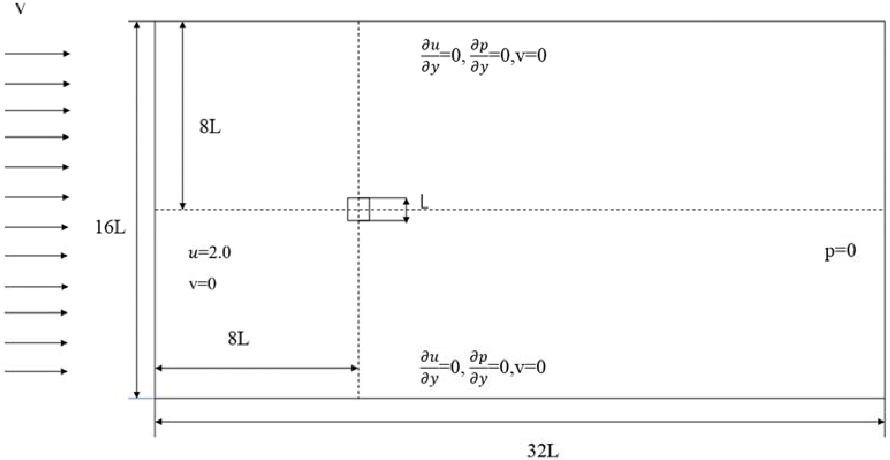
The simulation domain of flow over a square object is shown in Figure 2, in which the characteristic length L was set as 1, the side length of the square object was 1L, the size of the simulation domain was 32L × 16L, the incoming flow velocity $u$ was set as 2, and the Reynolds number was set as 2.2 × 10⁴. In addition, three grids, 200 × 400, 256 × 512, and 300 × 600, with different grid densities, were tested for the study of the grid independence in this calculation. The final results showed that the optimal number of grids was 256 × 512, which was applied in the following parametric studies. The time step dt and the number of iteration steps were set as 0.0005 s and 400,000, respectively.

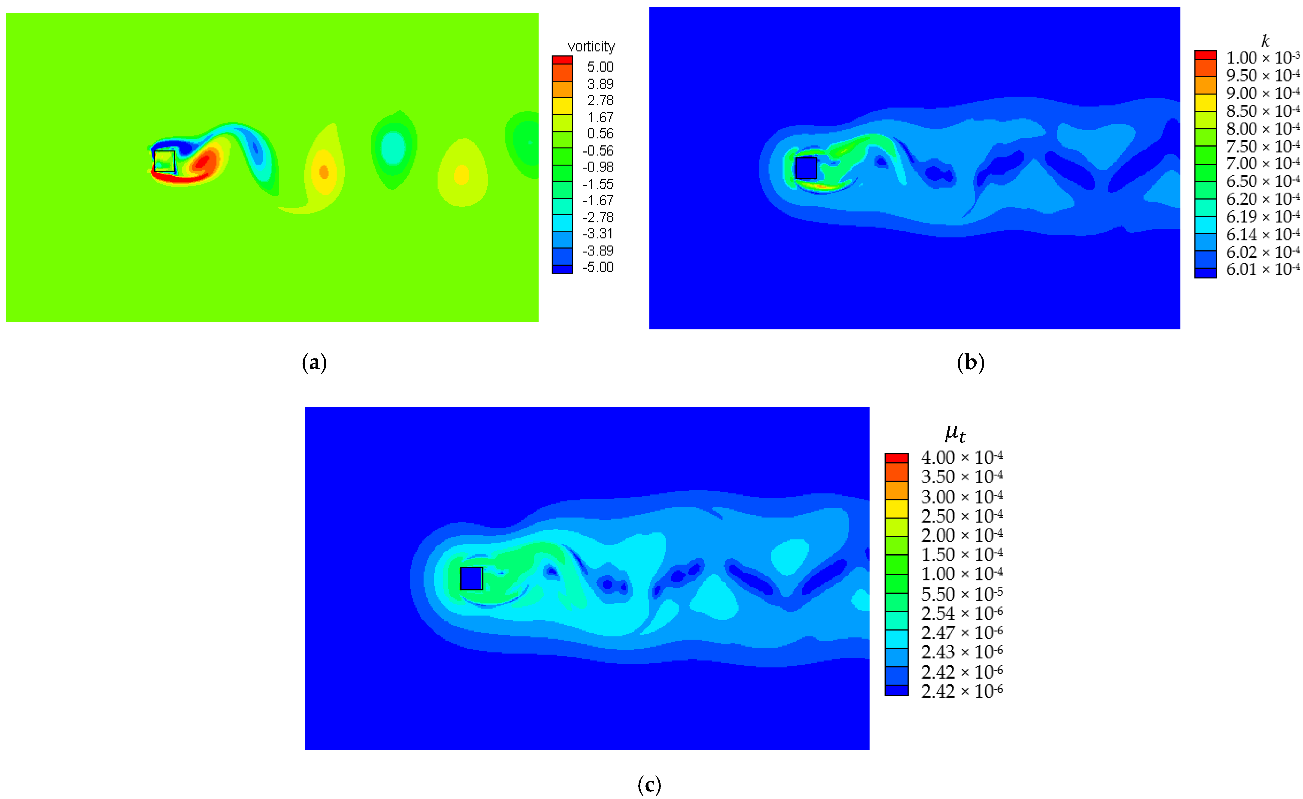
A series of contour plots are summarized in Figure 3 based on the simulation results. We observed that after the calculation convergence, distinct periodic falling vortexes, the so-called Carmen vortex Street, appeared behind the square object. The generation process of these vortexes was the essential factor causing the periodic oscillation of lifting resistance. Due to the large and unstable variations in the velocity of flow just outside the inner layer, the turbulent kinetic energy $k$ and the turbulent dissipation rate ε of the corresponding flow field in this area unstably increased.

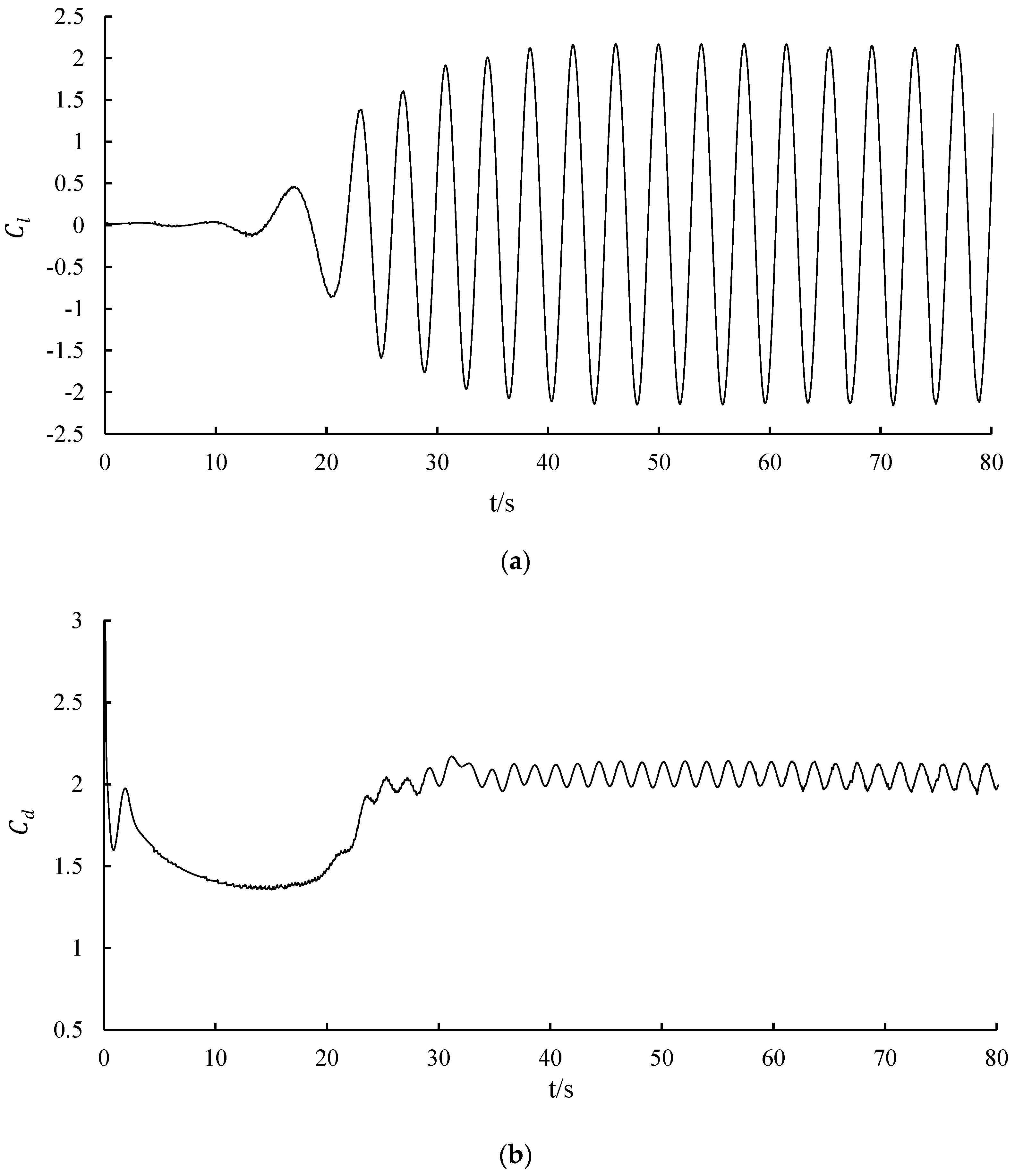
As shown in Figure 4, the resistance coefficient showed a downward trend at the beginning of the calculation, and the fluid flow was relatively stable during this period. The resistance coefficient rose sharply after 20 s because a large vortex was generated behind the square object. Meanwhile, the large vortex was about to fall off, which caused instability in the increased resistance. Because unstable vortices began to occur between 20 s and 35 s, an irregular numerical vibration of the resistance coefficient appeared accordingly. After 35 s, the fallout of the tail vortex gradually stabilized and thus produced a stable fluctuated lift and drag.

The simulation results are summarized and compared with reference [23] in

Table 1. Comparison with the reference.

/	${\mathit{C}}_{\mathit{l}}{}_{\mathit{m}\mathit{a}\mathit{x}}$	${\mathit{C}}_{\mathit{d}}$	St
This paper	2.14	2.05	0.135
Ref. [23]	2.05	2.11	0.14
Error	4.3%	2.8%	3.6%

. The resistance coefficient after convergence stabilized at 2.05, the error of which was only 2.8% compared with the previously reported resistance coefficient 2.11. The maximum lift coefficient was 2.14, and the corresponding error was only 4.3%. In addition, the Strouhal number was about 0.135, with an error of only 3.6%. Generally, the results achieved in this work are in good agreement with the reference and the corresponding maximum error is less than 5%, which verifies the feasibility and the accuracy of the proposed algorithm.

3.2. Models of Fish Motion

There are many movement modes of fish, including body/caudal (BCF) and middle paired-fin (MPF) swimming modes. Most fishes adopt BCF movement mode, which can be further classified into anguilliform, subcarangiform, carangiform, and thuniform according to different propulsion parts. The propulsion mode of the fish adopted in this work was the subcarangiform mode.

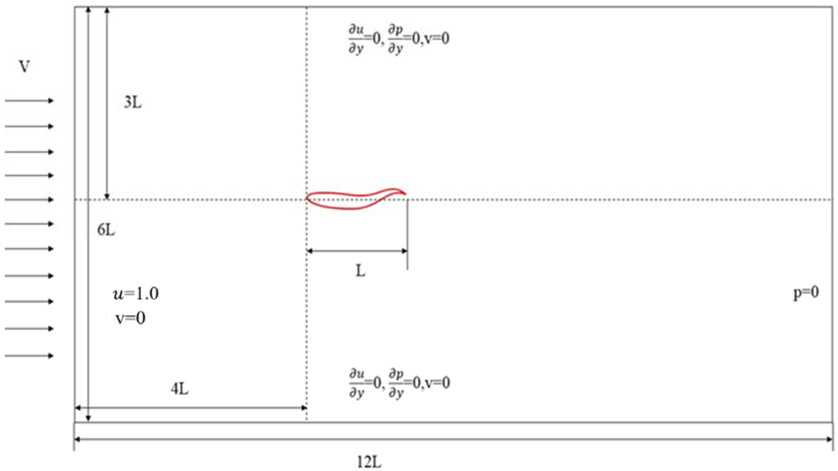
Three grids, 200 × 400, 256 × 512, and 300 × 600, were used to test the grid independence, and the grid of 256 × 512 was verified as the optimal one to be applied in the following parametric studies in this work. The shape of the fish was set as NACA0012, which is shown in Figure 5. The corresponding NACA0012 airfoil, as shown in Figure 6, was used as the contour of the fish-like robot. The length of the fish airfoil was set as L = 1, the size of the simulation domain was set as 6L × 12L, the vertex position of the fish was set at the location with coordinates of (4L, 3L), and the incoming flow velocity was set as v = 1. In addition, the x-direction was defined as the direction from the head to the tail of the fish.

The median line of fish moves along the normal direction of the fluid flow, and its motion equation is given as

$$y_o=A_m\left(x\right)\cos \left[2\pi \left(x-ct\right)+\varnothing \right]+d, 0\le x\le 1,$$

(29)

where A_m, c, $\varnothing$, and d represent the amplitude of the fish’s vibration, phase speed, phase position, and position of the middle line of the fish, respectively. In order to simulate the movement of the fish’s ridgeline more reasonably, the amplitude A_m can be approximated as a quadratic polynomial

$$A_m\left(x\right)=C_0+C_{1}x+C_2{x}^2$$

(30)

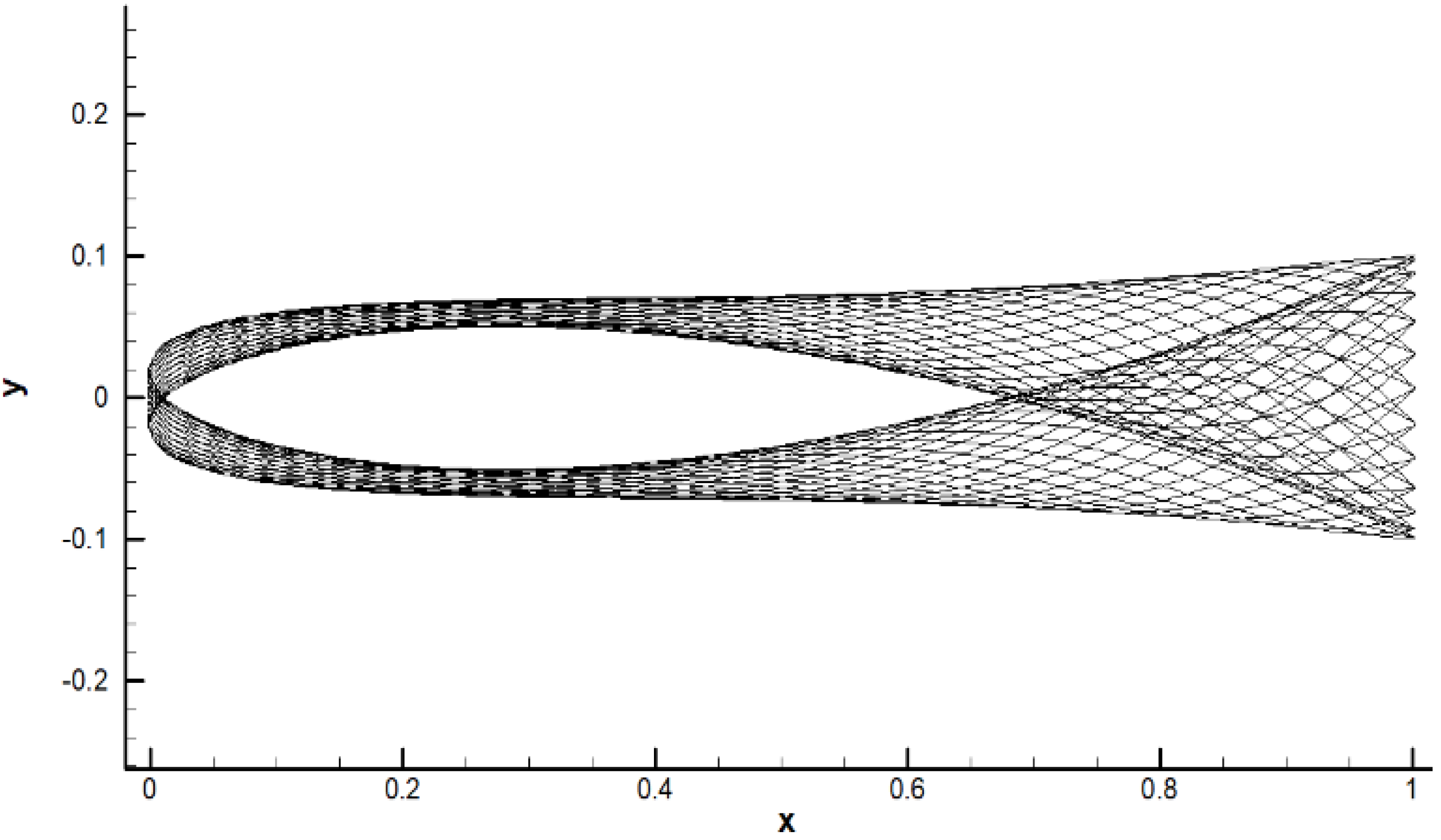
where $C_0$, $C_1$, and $C_2$ are the coefficients derived from the steady-state kinematics data [24]. According to $A_m\left(0\right)=0.02$,$A_m\left(0.1\right)=0.10$, and $A_m\left(0.2\right)=0.01$, those coefficients can be determined as $C_0=0.02$, $C_1=-0.0825$, and $C_2=0.1625$. The swing range is shown in Figure 7, which reasonably describes the lateral motion of the amplitude of the fish ridge during the swing. It should be noted that the length of the fish-like robot does not change during the wave-like forward movement. Only the fish body displaces and deforms in the lateral direction.

3.3. Influence of Different Reynolds Numbers

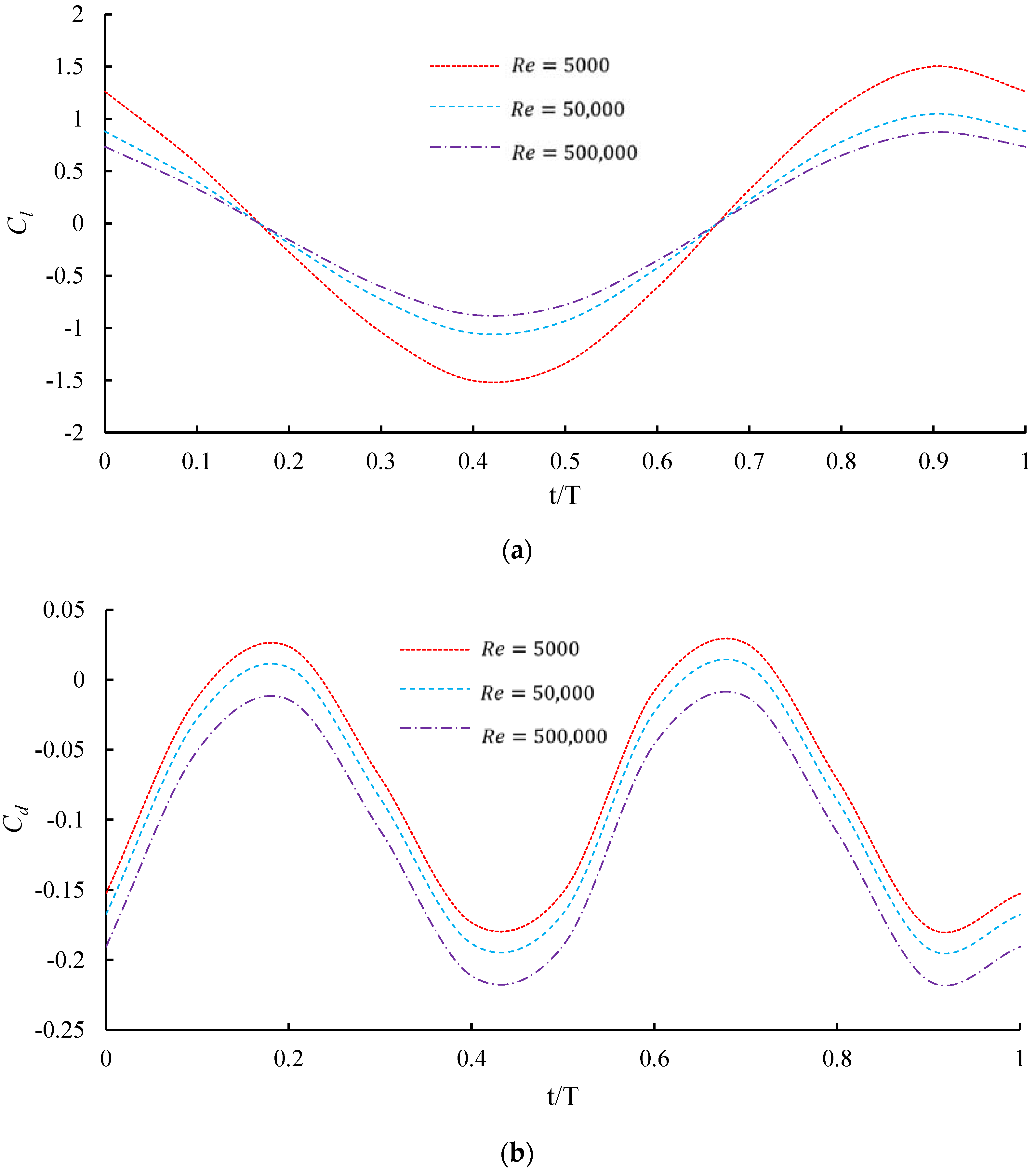
The flow fields induced by the swing of underwater fish-like robots normally have a high Reynolds number. In order to verify the characteristics of the induced flow field, we set up three fluid flows with three different Reynolds numbers, namely $5000$, $50,000$, and $500,000$, by modifying the fluid viscosity for a comparative study. The corresponding variation trends in lift and drag coefficients with the Reynolds numbers are summarized in Figure 8, which are consistent with those in real situations. It can be seen from the figure that the amplitude of the lift coefficient and the drag coefficient decrease with increasing Reynolds number. Consequently, the flow with a high Reynolds number can effectively reduce the lateral force coefficient of a fish-like robot and thus provide more thrust force.

Contours of vorticity induced by the swimming fish-like robot at different Reynolds numbers are shown in Figure 9. A remarkable reverse Karman vortex street appears behind the fish body, which is beneficial for the fish-like robot to swim forward. In addition, compared with the situation of low Reynolds numbers, the vortexes generated in the flow field with high Reynolds numbers are densely packed and, simultaneously, last for a relatively long period.

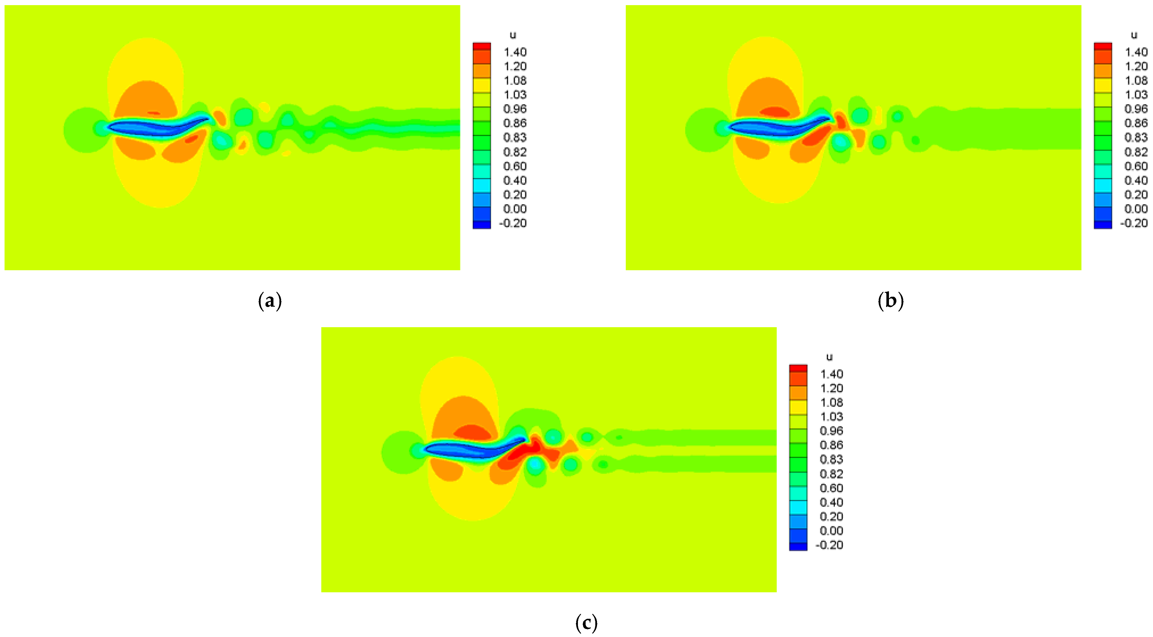
The contours of velocity along the x-direction at different Reynolds numbers are shown in Figure 10. In addition to the higher velocities around the middle section of the airfoil, relatively higher velocities also occur around the tail section, which is attributed to the higher instantaneous relative velocities between the tail section and the surrounding fluid during the movement. Furthermore, the location of the flow field with relatively higher velocity depends on the moving direction of the tail. Specifically, it is located nearby the lower surface of the tail section when the tail section moves downward and near the upper surface when the tail section moves upward. The obtained velocity field behind the airfoil at a higher Reynolds number is much higher than that at a lower Reynolds number. This jet flow with higher velocity gives rise to a higher thrust force by the fish-like robot swinging in fluid flow with a high Reynolds number.

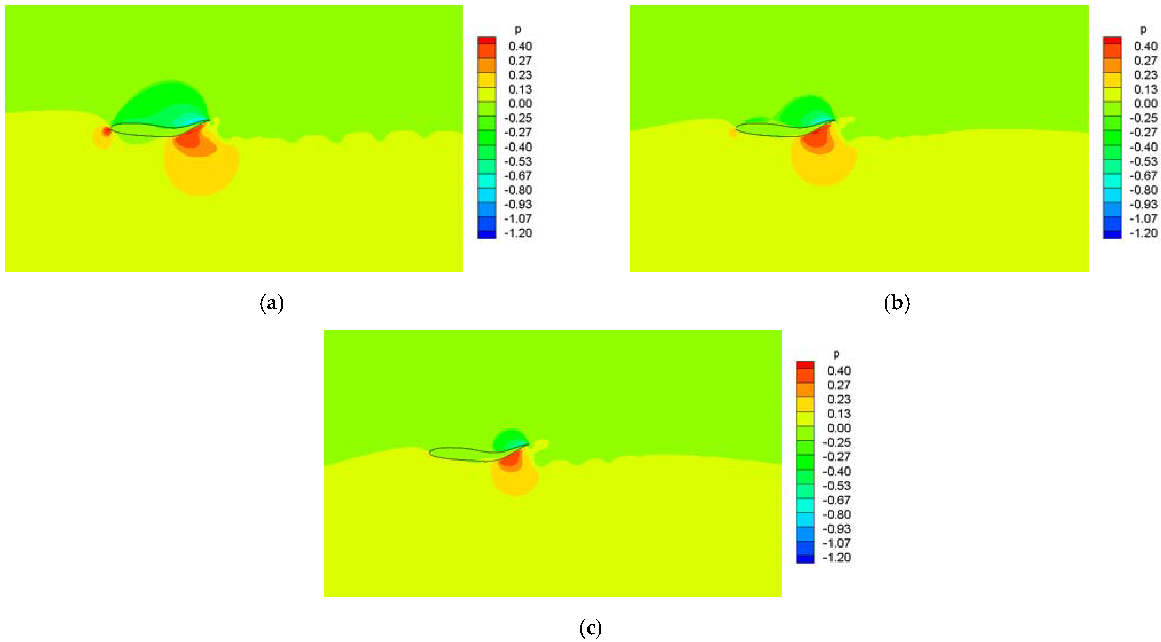
As shown in Figure 11, the pressure contours at different Reynolds numbers show that the incoming fluid flow induces high pressure nearby the airfoil head at all Reynolds numbers. Additionally, the swing of the tail creates a high-pressure region, which is attributed to the interaction between the motion of the tail and the surrounded fluid, and the high velocity induced by the swinging tail. Furthermore, the pressure nearby the tail at a high Reynolds number is lower than that at a low Reynolds number, which is one of the reasons for the low lift coefficient at a high Reynolds number.

Generally, the results and the corresponding analysis above prove that the lift and the drag coefficients of a fish-like robot can be reduced by increasing the Reynolds number. This is because, compared with the situation of a lower Reynolds number, a higher jet velocity around the tail region is induced at a higher Reynolds number and, thus, higher thrust force is generated. The enhanced thrust force gives rise to a reduced drag coefficient. In addition, a lower lift coefficient at a higher Reynolds number is achieved due to the lower pressure around the tail region.

4. Conclusions

In this work, the immersed boundary method was applied to the numerical simulation of a fish-like robot swinging in fluid. It can be tactfully applied to deal with turbulent flows of high Reynolds numbers by combining the k-ε turbulence model and the wall model. The proposed method was firstly verified by a flow over a square object at a high Reynolds number. A maximum error of only 4.3% of the parameters including the lift coefficient, the drag coefficient, and the Strouhal number was observed when comparing the results achieved by the proposed method with that achieved by the reference, which verified the accuracy and feasibility of the proposed algorithm. The swings of the fish-like robot at three different Reynolds numbers were then simulated and analyzed. We found that the maximum lift coefficient at a high Reynolds number is lower than that at a low Reynolds number. Therefore, the size of a fish-like robot can be appropriately increased during the design process to increase the Reynolds number.

References

1. Aracri, S.; Giorgio-Serchi, F.; Suaria, G.; Sayed, M.E.; Stokes, A.A. Soft robots for ocean exploration and offshore operations: A perspective. Soft Robot. 2021, 8, 625–639. [Google Scholar] [CrossRef] [PubMed]
2. Marcin, M.; Adam, S.; Jerzy, Z.; Marcin, M. Fish-like shaped robot for underwater surveillance and reconnaissance–Hull design and study of drag and noise. Ocean Eng. 2020, 217, 107889. [Google Scholar] [CrossRef]
3. Glaze, J.; Salazar, R.; Vasconcellos, R.; Abdelkefi, A. Comparative design, hydrodynamic analysis, and physical performance of fish-like robots. Appl. Ocean Res. 2020, 106, 102443. [Google Scholar] [CrossRef]
4. Chen, Y.; Qiao, J.; Liu, J.; Zhao, R.; An, D.; Wei, Y. Three-dimensional path following control system for net cage inspection using bionic robotic fish. Inf. Process. Agric 2021, 9, 2214–3173. [Google Scholar] [CrossRef]
5. Utter, B.; Brown, A. Open-source five degree of freedom motion platform for investigating fish-robot interaction. HardwareX 2020, 7, e00107. [Google Scholar] [CrossRef] [PubMed]
6. Shao, J.; Wang, L.; Yu, J. Development of an artificial fish-like robot and its application in cooperative transportation. Control Eng. Pract. 2008, 16, 569–584. [Google Scholar] [CrossRef]
7. Giorgio-Serchi, F.; Weymouth, G.D. Drag cancellation by added-mass pumping. J. JFM 2016, 798. [Google Scholar] [CrossRef] [Green Version]
8. Weymouth, G.; Giorgioserchi, F. Analytic Modeling of a Size-Changing Swimmer; Springer: Cham, Switzerland, 2018. [Google Scholar]
9. Armanini, C.; Farman, M.; Calisti, M.; Serchi, F.G.; Renda, F. Flagellate Underwater Robotics at Macroscale: Design, Modeling, and Characterization. IEEE Trans. Robot. 2021, 38, 731–747. [Google Scholar] [CrossRef]
10. Liu, H.; Wassersug, R.J.; Kawachi, K.A. Computational fluid dynamics study of tadpole swimming. J. Exp. Biol. 1996, 199, 1245–1260. [Google Scholar] [CrossRef] [PubMed]
11. Liu, H.; Wassersug, R.J.; Kawachi, K.A. The three-dimensional hydrodynamics of tadpole locomotion. J. Exp. Biol 1997, 200, 2807–2819. [Google Scholar] [CrossRef] [PubMed]
12. Liu, H.; Ellington, C.P.; Kawachi, K.A.; Berg, C.V.D.; Willmott, A.P. A computational fluid dynamic study of hawkmoth hovering. J. Exp. Biol. 1998, 201, 461–477. [Google Scholar] [CrossRef] [PubMed]
13. Carling, J.; Williams, T.; Bowtell, G. Self-propelled anguilliform swimming: Simultaneous solution of the two-dimensional Navier–Stokes equations and Newton’s laws of motion. J. Exp. Biol. 1998, 201, 3143–3166. [Google Scholar] [CrossRef] [PubMed]
14. Togashi, F.; Ito, Y.; Murayama, M. Flow Simulation of flapping Wings of an Insect Using OVERSET unstructured Grid. In Proceedings of the Aiaa Computational Fluid Dynamics Conference, San Diego, CA, USA, 24–27 June 2013. [Google Scholar]
15. Zhang, L.P.; Chang, X.H.; Duan, X.P.; Wang, Z.Y.; Zhang, H.X. A block LU-SGS implicit unsteady incompressible flow solver on hybrid dynamic grids for 2D external bio-fluid simulations. Comput. Fluids 2009, 38, 290–308. [Google Scholar] [CrossRef]
16. Maertens, A.P.; Triantafyllou, M.S.; Yue, D. Efficiency of Fish Propulsion. Bioinspiration Biomim. 2015, 10, 4. [Google Scholar] [CrossRef] [PubMed] [Green Version]
17. Peskin, C.S. Flow patterns around heart valves: A numerical method. J. Comput. Phys. 1972, 10, 252–271. [Google Scholar] [CrossRef]
18. Weymouth, G.D.; Yue, K.P. Conservative Volume-of-Fluid method for free-surface simulations on Cartesian-grids. J. Comput. Phys. 2010, 229, 2853–2865. [Google Scholar] [CrossRef]
19. Noor, D.Z.; Chern, M.J.; Horng, T.L. An immersed boundary method to solve fluid–solid interaction problems. Comput. Mechv. 2009, 44, 447–453. [Google Scholar] [CrossRef]
20. Kress, R. Linear Integral Equations. Ann. Math. 2014, 82, 323–349. [Google Scholar]
21. Pironneau, O. Analysis of the K-Epsilon Turbulence Model; Wiley: Hoboken, NJ, USA, 1993. [Google Scholar]
22. Griebel, M.; Dornseifer, T.; Neunhoeffer, T. Numerical Simulation in Fluid Dynamics: A Practical Introduction; Society for Industrial and Applied Mathematics: Phidadelphia, PA, USA, 1998. [Google Scholar]
23. Mohammadi, B.; Pironneau, O. Unsteady separated turbulent flows computation with wall-laws and k–ε model. Comput. Methods Appl. Mech. Eng. 1997, 148, 393–405. [Google Scholar] [CrossRef]
24. Wardle, C.S.; Videler, J.J. Fish Swimming; Cambridge University Press: Britain, UK, 1980. [Google Scholar]
Figure 1. Schematic diagram of virtual boundary layer.
Actuators 11 00158 g001
Figure 2. Simulation domain of flow over a square object.
Actuators 11 00158 g002
Figure 3. Contours of vorticity, turbulent kinetic energy, and turbulent dissipation. (a) Vorticity; (b) turbulent kinetic energy; (c) turbulent dissipation rate.
Actuators 11 00158 g003
Figure 4. The lift and the drag coefficients of the flow over a square object. (a) The lift coefficient C l ; (b) the drag coefficient Cd.
Actuators 11 00158 g004
Figure 5. Fish body appearance model.
Actuators 11 00158 g005
Figure 6. Simulation domain and the corresponding boundary conditions.
Actuators 11 00158 g006
Figure 7. Length and swing range of the fish-like robot.
Actuators 11 00158 g007
Figure 8. Lift and drag coefficients at different Reynolds numbers. (a) The lift coefficient C l ; (b) the drag coefficient Cd.
Actuators 11 00158 g008
Figure 9. Contours of vorticity at different Reynolds numbers. (a) R e = 5000 ; (b) R e = 50 , 000 ; (c) R e = 500 , 000 .
Actuators 11 00158 g009
Figure 10. Contours of velocity along x-direction at different Reynolds numbers. (a) R e = 5000 ; (b) R e = 50 , 000 ; (c) R e = 500 , 000 .
Actuators 11 00158 g010
Figure 11. Pressure contours at different Reynolds numbers. (a) R e = 5000 ; (b) R e = 50 , 000 ; (c) R e = 500 , 000 .
Actuators 11 00158 g011