Fault-Tolerant Control of Skid Steering Vehicles Based on Meta-Reinforcement Learning with Situation Embedding

Abstract

Meta-reinforcement learning (meta-RL), used in the fault-tolerant control (FTC) problem, learns a meta-trained model from a set of fault situations that have a high-level similarity. However, in the real world, skid-steering vehicles might experience different types of fault situations. The use of a single initial meta-trained model limits the ability to learn different types of fault situations that do not possess a strong similarity. In this paper, we propose a novel FTC method to mitigate this limitation, by meta-training multiple initial meta-trained models and selecting the most suitable model to adapt to the fault situation. The proposed FTC method is based on the meta deep deterministic policy gradient (meta-DDPG) algorithm, which includes an offline stage and an online stage. In the offline stage, we first train multiple meta-trained models corresponding to different types of fault situations, and then a situation embedding model is trained with the state-transition data generated from meta-trained models. In the online stage, the most suitable meta-trained model is selected to adapt to the current fault situation. The simulation results demonstrate that the proposed FTC method allows skid-steering vehicles to adapt to different types of fault situations stably, while requiring significantly fewer fine-tuning steps than the baseline.

1. Introduction

Due to their simple mechanical structure and flexible control, skid-steering distributed drive vehicles have been widely applied in various scenarios, including wheeled robots [1,2], agricultural vehicles [3], military vehicles [4,5], and so on. Generally, a skid-steering vehicle has four independent driving wheels, forming a redundant actuator system, which delivers remarkable maneuverability and more options for FTC methods [6]. With the development of meta-RL algorithms, some recent studies applied meta-RL algorithms to the FTC problem of actuator faults, providing new insights into the FTC mechanism of skid-steering vehicles [7,8]. Meta-RL learns an initial meta-trained model from a set of fault situations that have high-level similarity. However, in the real world, skid-steering vehicles might experience different types of fault situations, where the dynamical models can be significantly different from one another [9]. The single initial meta-trained model in conventional meta-RL algorithms limits the ability to learn fault situations that do not have strong similarity to the learned faults, leading to low generalizability to novel fault situations [10,11].

Meta-RL approaches were successfully applied to adapt to system failures and external disturbances, especially the most representative model-agnostic meta-learning (MAML) [12]. In [13,14,15,16], the authors presented a series of methods based on meta-RL to quickly adapt their control policies to maintain degraded performance when faults occur in aircraft fuel transfer systems. The scheme of FTC methods includes offline meta-training and online meta-testing stages. In [17], the authors presented a reference trajectory update method based on meta-RL, to improve the trajectory tracking performance of unmanned aerial vehicles (UAVs) under actuator faults and disturbances. They leveraged meta-RL to quickly adapt the system model at runtime, as well as to update the reference trajectory without needing access to the control inputs. In [18], an impact-angle guidance law was proposed for the interception of a maneuvering target using a varying velocity interceptor under partial actuator failures, based on meta-RL and model predictive path integral (MPPI). The deep neural dynamic can learn the changes and perturbations in the environment through the online adaption ability of meta-learning, which endows the proposed method with better tracking performance than the standard MPPI method. In [19], an adaptive controller based on meta-RL was proposed for automatic train velocity regulation. The velocity regulation problem, under the complicated railway environment and uncertain dynamics of the system, is expressed as a sequence of stationary Markov decision process (MDP) with unknown transition probabilities. The meta-RL algorithm learns to track the desired speed under changing conditions. In [20], the authors proposed meta twin-delayed deep deterministic policy gradient (meta-TD3) to realize the control of UAVs, allowing the UAVs to quickly track a target characterized by uncertain motion. As meta-RL showed great potential in quickly adapting to system failures and external disturbances in recent years, it can provides new insights into the FTC problem of skid-steering vehicles and, as such, is incorporated into our work.

A major limitation of conventional meta-RL methods is that they seek a common initialization in the entire task distribution, which substantially limits their application in multi-task distribution [21,22]. To mitigate this limitation, some methods have extended MAML with the capability to identify the mode of tasks sampled from a multi-modal task distribution. In [23,24], the authors developed a Multi-Modal Model-Agnostic Meta-Learner (MuMoMAML). The model-based learner first effectively recognizes the mode of the task distribution through a few samples from the target task, and then adapts to the target task through gradient updates. In [25], the authors introduced a task encoder into the meta-RL framework and developed a new meta-RL method; namely TESP. TESP trains a shared policy and a stochastic gradient descent (SGD) optimizer coupled to a task encoder network from a set of tasks. The SGD optimizer is applied to quickly learn a task encoder for each task, which generates the corresponding task embedding based on past experience. Meanwhile, the shared policy is learned across all tasks and conditioned on task embeddings. To exploit information about task relationship, in [26], the authors proposed a task embedding of visual classification tasks, named Task2Vec, which provides a fixed-dimensional embedding of the task that is independent of details and does not require any understanding of the class label semantics. In [27], the authors proposed a novel representation, named MATE (model-aware task embedding), which is able to efficiently fuse the data distribution and model inductive bias. MATE introduces a model-dependent surrogate function to improve the current kernel mean embedding, which can be incorporated into deep neural networks. In [28], the authors proposed an algorithm called FAMLE to learn the multi-modal task distribution by meta-training several initial models and allowing the robot to select the most suitable initial model as the starting point to adapt to the current situation. FAMLE leverages the embedding of the meta-trained models to select the starting point, making it able to adapt faster than a single meta-trained model. In fact, our method uses FAMLE as the situation-embedding model, to select the most suitable meta-trained model for the fault situation of a skid-steering vehicle as a starting point for online adaption.

The main purpose of this study is to develop an FTC method based on meta-RL which allows skid-steering vehicles to adapt to different types of fault situations. From the analysis above, meta-training multiple initial models and selecting the most suitable one could more quickly and better optimize a policy for the fault situation than using a single initial meta-trained model. The questions that arise here are how to meta-train multiple initial meta-trained models and how to select the most suitable one among them, based on the online dataset.

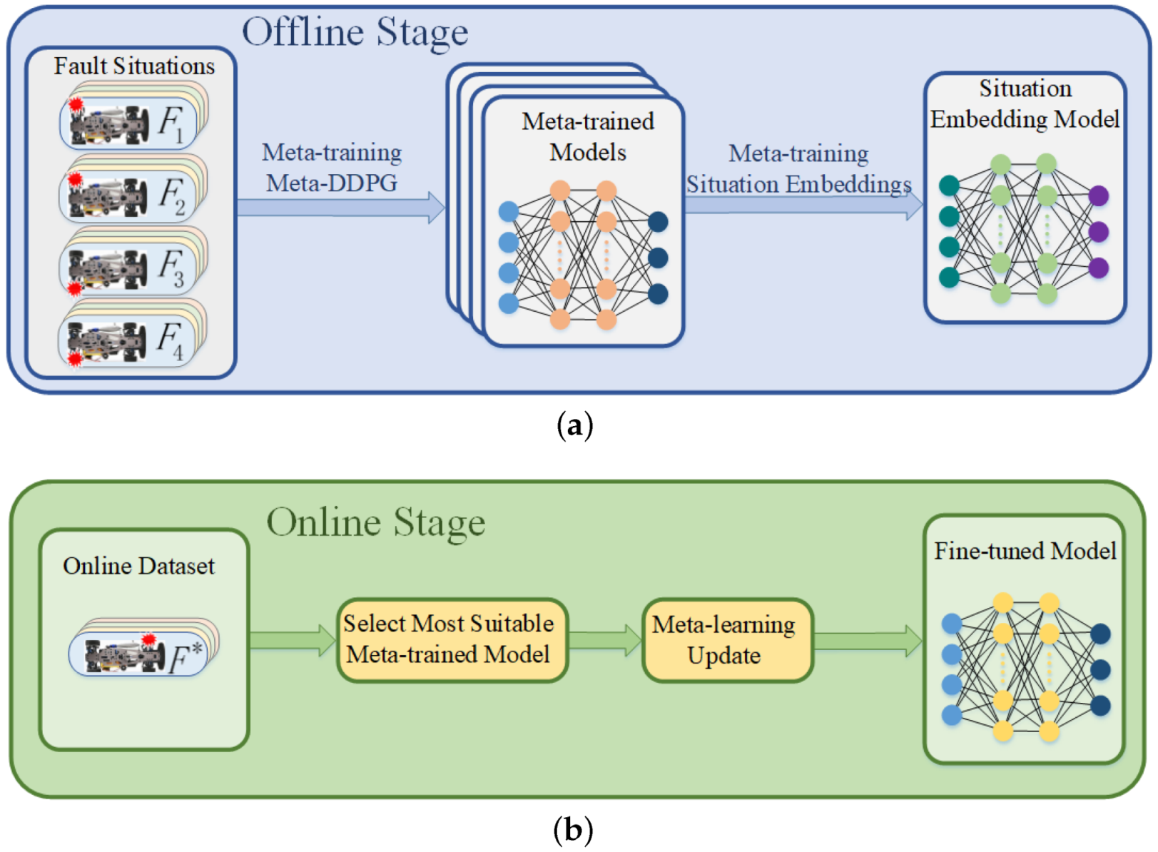
Based on the above motivation, we introduce a situation embedding model into the current meta-DDPG-based FTC framework, and develop a new FTC method, which achieves better performance on adapting different types of fault situations; namely meta-DDPGSE (meta-DDPG with situation embedding). The situation embedding model generates a d-dimensional vector, which is a specific parameter of meta-trained models, named situation-embeddings. We first apply the meta-DDPG algorithm to train multiple meta-trained models for different types of fault situations. Then, states and actions generated from the meta-trained models under the corresponding fault situations are used as the input for the situation embedding model in the offline stage. We can use the online data set as input for the situation embedding model, to select the most suitable meta-trained model for current fault situation as the starting point for online adaptation. In summary, we combine the meta-DDPG algorithm and the situation embedding model to facilitate rapid adaptation to the fault situation through selection of the most suitable initial meta-trained model.

The main contributions of this study are as follows: (1) We develop a meta-DDPGSE-based FTC method for skid steering vehicles, which achieves high performance on different types of fault situations; (2) a situation embedding model is introduced into the conventional meta-RL-based FTC framework, in order to select the most suitable meta-trained model for the current fault situation; and (3) selecting the most suitable meta-trained model based on online data set allows the agent to quickly adapt the policy to different types of fault situations. To the best of our knowledge, this is the first work to introduce the situation embedding model into the meta-RL-based FTC framework and apply it to the FTC problem of skid-steering vehicles.

The remainder of this paper is structured as follows. Section 2 introduces the torque distribution agent design and the problem formulation for the meta-DDPGSE-based FTC method. Section 3 provides the framework of the meta-DDPGSE-based FTC method. In Section 4, the simulation environment and setting are detailed. We validate the proposed method with simulation in Section 5. Finally, our conclusions are provided in Section 6.

2. Preliminaries

2.1. DDPG-Based Skid-Steering Vehicle Control Method

The DDPG algorithm is adopted in this work to learn the control policy for skid-steering vehicles. The DDPG algorithm has a continuous action space, which is very suitable for applications in complex continuous action control processes [29,30,31,32].

As an Actor–Critic algorithm, the DDPG algorithm includes a Critic network and Actor network [33,34]. The Critic network $Q(s,a|{\theta }^Q)$ can evaluate the value of taking an action a in state s, while the Actor network $\mu \left(s\right|{\theta }^{\mu })$ is a function used to map a state s to a deterministic policy a, where ${\theta }^Q$ and ${\theta }^{\mu }$ are the network parameters. The DDPG is a model-free, off-policy algorithm, and the design of the agent’s state space, action space, and reward function have important impacts in the performance of the skid-steering vehicle [35].

2.1.1. State Space

The control objective is the actual longitudinal speed and yaw rate, used to track the desired value accurately and effectively. The state space includes the error of longitudinal speed $v_{delta}$ and yaw rate ${\omega }_{delta}$, which are defined as:

$$\begin{array}{cc}\hfill v_{delta}& =v_{xd}-v_{xa},\hfill \\ \hfill {\omega }_{delta}& ={\omega }_{\varphi d}-{\omega }_{\varphi a},\hfill \end{array}$$

(1)

where $v_{xd}$ and ${\omega }_{\varphi d}$ are the desired values of the longitudinal speed and yaw rate, respectively; and $v_{xa}$ and ${\omega }_{\varphi a}$ are the corresponding actual values, respectively. The desired and actual values are depicted in Figure 1. The longitudinal acceleration, $v_{xa}^{\prime }$, and the angular acceleration, ${\omega }_{\varphi a}^{\prime }$, are also used as variables of the state space, which seriously affect the vehicle’s maneuverability. The state space is defined as follows:

$$state=\left\{v_{delta},{\omega }_{delta},v_{xa}^{\prime },{\omega }_{\varphi a}^{\prime }\right\}.$$

(2)

2.1.2. Action Space

A vehicle’s behavior depends on the driving torque on its wheels, its geometry, and the ground. It is assumed in this study that the geometry and the ground do not change. Therefore, the driving torque on each wheel is used as an action space variable. Thus, the action space is defined as follows:

$$action=\left\{T_{fl},T_{rl},T_{fr},T_{rr}\right\}.$$

(3)

In the learning process of RL, the agent can only select actions based on the randomly generated policy, and then optimize the policy through ’trial and error’. This action selection method is likely to generate a low reward at the beginning, and may also lead to sub-optimal policy actions due to insufficient exploration. Therefore, we use an assisted controller to generate reference operations within an acceptable time. We call this reference operation as the criteria action.

The key point is to use the criteria action to assist the agent at the beginning of the learning process, then eliminate such assistance when the agent can find a safe area. Here, the agent’s action choice is defined as the agent action, and the real action signal sent to the system is the execution action.

$$a_e=\left(1-{\gamma }^i\right)·a_a+{\gamma }^i·a_c,$$

(4)

where $\gamma$ is the discount factor and i is the iteration episode. $a_e$ is execution action, $a_a$ is agent action and $a_c$ is criteria action. This is the same as training the agent with an inaccurate controller first. After a period of assistance, the agent can select actions independently. This provides the agent with a search direction and accelerate the learning process. The assisted controller is defined as follows:

$$\begin{array}{c}\hfill T_{lf}=T_{lr}=K_p\left(m·\frac{v_{delta}}{dt}\right)-J·\frac{{\omega }_{delta}}{dt},\\ \hfill T_{rf}=T_{rr}=K_p\left(m·\frac{v_{delta}}{dt}\right)+J·\frac{{\omega }_{delta}}{dt},\end{array}$$

(5)

where $K_p$ is the proportional coefficient and $dt$ is the time step.

2.1.3. Reward Function

The reward function acts as a signal to evaluate the performance when taking an action a when in state s. Rewards are the only feedback signals available for the agent’s learning. Reasonably designing the reward function is the key to guiding the agent to obtain an effective control policy. Design of the reward function is mainly based on the vehicle’s maneuverability, which is reflected in reducing errors related to longitudinal speeds and yaw rates. Therefore, to ensure the performance of the vehicle, a well-defined reward function provided at every time step is introduced:

$$\begin{array}{cc}\hfill R=& -\left(v_{delta}^2+5\times {\omega }_{delta}^2\right)-0.01\times \left({\left(v_{xa}^{\prime }\right)}^2+{\left({\omega }_{\varphi a}^{\prime }\right)}^2\right)\hfill \\ \hfill & -0.001\times \left(T_{fl}^2+T_{rl}^2+T_{fr}^2+T_{rr}^2\right)+D.\hfill \end{array}$$

(6)

The first term in the reward function above encourages the agent to minimize errors with longitudinal speeds and yaw rates. The second and third terms in the reward function encourage the agent to reduce the action value when the error is within a certain range, to prevent the error from not converging. The last term is a large positive reward when the agent is close to the ideal conditions, and is defined as below:

$$D=\left\{\begin{array}{cc}3000,\hfill & if\left|v_{delta}\right|<0.01\times \left|v_{xd}\right|and\left|{\omega }_{delta}\right|<0.01\times \left|{\omega }_{\varphi d}\right|\hfill \\ 0,\hfill & otherwise.\hfill \end{array}\right.$$

(7)

In this way, a large positive reward is applied when the agent is close to the ideal conditions.

2.2. Problem Formulation: Meta-DDPGSE-Based FTC Method

Our approach mirrors the MAML algorithm, and the whole process of the FTC method is split into two steps: meta-training in the offline stage and meta-testing in the online stage [36].

In the offline stage, we first train multiple meta-trained models for different types of fault situations. For each fault situation $F_i$, we consider a meta-trained model, expressed as a function $f_{{\theta }_i}$. During meta-training, the parameters ${\theta }_i$ are initialized randomly and updated to ${\theta }_{ij}^{\prime }$ while adapting to fault $F_i^j$:

$${\theta }_{ij}^{{}^{\prime }}={\theta }_i-\alpha {\nabla }_{{\theta }_i}{L}_{F_i^j}\left(f_{{\theta }_i}\right).$$

(8)

Meta-optimization is conducted across the faults. Then, the model parameters are updated according to Equation (9):

$${\theta }_i\leftarrow {\theta }_i-\beta {\nabla }_{{\theta }_i}\sum _{F_i^j\subset F_i}{L}_{F_i^j}\left(f_{{\theta }_{ij}^{\prime }}\right),$$

(9)

where $\alpha$ and $\beta$ are hyper-parameters for the optimization step size and L is the loss function of the DDPG algorithm.

The situation embeddings are vectors representing characteristics of multiple meta-trained models, which are used to select the most suitable model among them. We consider the situation embedding model as a function $f_{{\theta }_s}\left(s_{t+1}|s_t,a_t,h\right)$, where $s_{t+1}$, $s_t$, $a_t$, and h are the next state, the state, the action, and the situation embedding corresponding to the current fault situation, respectively. We collect the state-transition data ${\mathcal{D}}_{F_i}$ from each type of fault situation $F_{i=1:N}$ and construct a data set $\mathbb{D}$. Then, corresponding to each type of fault situation $F_{i=1:N}$, the situation embeddings $\mathbb{H}=\left\{h_{F_i}\right|i=1,\cdots ,N\}$ and model parameters ${\theta }_s$ are randomly initialized. The negative log-likelihood loss is calculated as:

$${\mathcal{L}}_{{\mathcal{D}}_{F_i}}\left({\theta }_s,h_{F_{i=1:N}}\right)={\mathbb{E}}_{{\mathcal{D}}_{F_i}}\left[-\log f_{{\theta }_s}\left(s_{s+1}|s_t,a_t,h_{F_i}\right)\right].$$

(10)

We train the situation embedding model to obtain the initial model parameters ${\theta }_s$ and situation embeddings $\mathbb{H}$. Through the combination of the situation embeddings $\mathbb{H}$ and parameters ${\theta }_s$, the situation embedding model could serve for N types of fault situations, in order to select the most suitable initial meta-trained model.

In the online stage, we first collect the data set of the vehicle operating under fault situations, then compute the likelihood of each situation embedding in $\mathbb{H}$, and select the meta-trained model that maximizes the likelihood of the recent data set. To be more precise, if $D_{online}$ is the recent data set, then:

$$h_{Likely}=arg\underset{h\in \mathbb{H}}{\max }{\mathbb{E}}_{D_{online}}\left[\log f_{{\theta }_s}\left(s_{t+1}|s_t,a_t,h\right)\right].$$

(11)

With the selected meta-trained model as the starting point, the agent is able to quickly adapt its policy to the current fault situation.

Based on the description of meta-DDPGSE-based FTC method above, the process is as follows: The FTC step begins with an abrupt fault, causing a discontinuous change in process dynamics $p\to p^{*}$. In the aftermath of the fault, the agent continues to interact with $p^{*}$, and records states, actions, and rewards in an online memory buffer $D_{online}$ using its current policy parameters $\theta$. Once sufficient interactions have been buffered, the likelihood of the recent observations for each situation embedding in $\mathbb{H}$ are computed. Then, we select the most suitable meta-trained model to adapt to the current fault situation, while obtaining a fine-tuned model with updated parameters ${\theta }^{*}$. The fine-tuned model is then used to distribute the driving torque under the current fault situation. The flowchart of the proposed FTC method is shown in Figure 2.

3. Meta-DDPGSE-Based FTC Method

The proposed FTC method includes offline and online stages. In the offline stage, we apply the meta-DDPG algorithm to train the corresponding meta-trained models with respect to N different types of fault situations. The situation embedding model is trained using the state-transition data generated from the meta-trained models. In the online stage, the agent collects sufficient interactions after a fault situation occurs, and then selects the most suitable meta-trained model to adapt the current fault situation. Finally, a fine-tuned model is obtained and applied to distribute the driving torque in the fault situation. The framework of the meta-DDPGSE-based FTC method is demonstrated in Figure 3.

3.1. Meta-Training of Meta-DDPG

In this work, meta-training of meta-DDPG is a process used to learn different types of fault situations and obtain meta-trained models corresponding to fault situations. In each type of fault situation, meta-training mainly includes two update processes: Internal RL for a single fault and external meta-learning update for multiple different faults. The faults in meta-training are randomly selected from the same type of fault situation. In the meta-DDPG algorithm, internal DDPG training and external meta-learning updating are performed alternately, meeting a certain update frequency. Internal DDPG learns multiple faults separately to obtain different parameters, and external meta-learning obtains the initial parameters of meta-DDPG by optimizing these different parameters.

In each type of fault situation $F_i$, we consider a function $f_{{\theta }_i}$ with parameters ${\theta }_i$ that is a policy for mapping a state s to an action a. When a new fault $F_i^j$ in the fault situation $F_i$ occurs, the policy function adapts to the new fault, and the parameters ${\theta }_i$ becomes ${\theta }_{ij}^{\prime }$ through the one-step gradient descent.

$${\theta }_{ij}^{\prime }={\theta }_i-\alpha {\nabla }_{{\theta }_i}{L}_{F_i^j}\left(f_{{\theta }_i}\right),$$

(12)

where $\alpha$ is the step size. The initial parameters ${\theta }_i$ are trained by optimizing for the average loss of the adapted policy $f_{{\theta }_{ij}^{\prime }}$ across faults sampled from $p\left(F_i\right)$. The meta-objective is as follows:

$$\underset{{\theta }_i}{min}\sum _{F_i^j\sim p\left(F_i\right)}{L}_{F_i^j}\left(f_{{\theta }_{ij}^{\prime }}\right)=\underset{{\theta }_i}{min}\sum _{F_i^j\sim p\left(F_i\right)}{L}_{F_i^j}\left({\theta }_i-\alpha {\nabla }_{{\theta }_i}{L}_{F_i^j}\left(f_{{\theta }_i}\right)\right).$$

(13)

Meta-optimization is used to optimize the initial policy parameters, such that only a few gradient steps produce a maximally effective policy on the new fault. The meta-optimization formula is as follows:

$${\theta }_i\leftarrow {\theta }_i-\beta {\nabla }_{{\theta }_i}\sum _{F_i^j\sim p\left(F_i\right)}{L}_{F_i^j}\left(f_{{\theta }_{ij}^{\prime }}\right),$$

(14)

where $\beta$ is the meta step size and $L_{F_i^j}$ is the loss function, which corresponds to the reward function in the RL; its formula is given as:

$$L_{F_i^j}\left(f_{{\theta }_i}\right)=-E_{s,a\sim f_{{\theta }_i}}\left[\sum _{t=1}{R}_i\left(s_t,a_t\right)\right].$$

(15)

The meta-training process of the fault situation $F_i$ is described in Algorithm 1.

Algorithm 1 Meta-training of meta-DDPG algorithm in fault situation $F_i$.

1: Randomly initialize critic network and actor network with weights ${\theta }_i^Q$ and ${\theta }_i^{\mu }$;

2: for$meta\_iteration=1,2,\cdots ,M$do

3:    Initialize a random fault $F_i^j\sim p\left(F_i\right)$;

4:    for $t=1,2,\cdots ,N$ do

5:        Sample trajectories from $F_i^j$ using policy $f_{{\theta }_i}$;

6:        Calculate the meta-learning loss function of fault $F_i^j$:

$L_{F_i^j}\left(f_{{\theta }_i}\right)=-E_{s,a\sim f_{{\theta }_i}}\left[{\sum }_{t=1}{R}_i\left(s_t,a_t\right)\right]$;

7:        Update the adapted parameters with gradient descent: ${\theta }_{ij}^{\prime }={\theta }_i-\alpha {\nabla }_{{\theta }_i}{L}_{F_i^j}\left(f_{{\theta }_i}\right)$;

8:        Sample trajectories using the adapted policy $f_{{\theta }_{ij}^{\prime }}$ in $F_i^j$;

9:        end for

10:    Meta-update ${\theta }_i\leftarrow {\theta }_i-\beta {\nabla }_{{\theta }_i}{\sum }_{F_i^j\sim p\left(F_i\right)}{L}_{F_i^j}\left(f_{{\theta }_{ij}^{\prime }}\right)$;

11: end for

3.2. Training the Situation Embedding Model

In this work, training of the situation embedding model is a process carried out to learn the characteristics of meta-trained models from the data set $\mathbb{D}$, which is generated from multiple meta-trained models. The initial model parameters ${\theta }_s$ and situation embeddings $\mathbb{H}$ are obtained by training the situation embedding model.

We consider the situation embedding model as a function $f_{{\theta }_s}\left(s_{t+1}|s_t,a_t,h\right)$ that predicts the next state, where $s_{t+1}$, $s_t$, $a_t$, and h are the next state, the current state, the current action, and the situation embedding of the current fault situation, respectively. For each type of sampled fault situation $F_{i=1:N}$, we randomly initialize the situation embedding $\mathbb{H}=\left\{h_{F_i}\right|i=1,\cdots ,N\}$ and the model parameters ${\theta }_s$. Then, the loss function for any type of fault situation $F_i\in \mathbb{F}$ is as follows:

$${\mathcal{L}}_{{\mathcal{D}}_{F_i}}\left({\theta }_s,h_{F_{i=1:N}}\right)={\mathbb{E}}_{{\mathcal{D}}_{F_i}}\left[-\log f_{{\theta }_s}\left(s_{s+1}|s_t,a_t,h_{F_i}\right)\right].$$

(16)

The training objective of the situation embedding model is to find the initial model parameters ${\theta }_s$ and situation embedding $\mathbb{H}$. We consider this process as a meta-optimization problem, defined as follows:

$${\theta }_s,\mathbb{H}=\arg \underset{{\theta }_s,F_{i=1:N}}{\min }{\mathbb{E}}_{F_i\sim \mathbb{F}}\left[{\mathcal{L}}_{{\mathcal{D}}_{F_i}}\left(U_{F_i}^k\left({\theta }_s,h_{F_i}\right)\right)\right],$$

(17)

where $U_{F_i}^k\left(·,·\right)$  represents the gradient descent update rule for k gradient descent steps. For any type of fault situation $F_i\in \mathbb{F}$, we use the update rule to update the parameters of the situation embedding model, including the parameters ${\theta }_s$ and the situation embedding $h_{F_i}$. At each update step, we randomly choose a fault situation $F_i$ from $\mathbb{F}$, and update the parameters ${\theta }_s$ and situation embedding $h_{F_i}$ simultaneously, through use of the following formula:

$$\begin{array}{cc}\hfill {\tilde{\theta }}_s,{\tilde{h}}_{F_i}& =U_{F_i}^k\left({\theta }_s,h_{F_i}\right)\hfill \\ \hfill {\theta }_s& :={\theta }_s+{\alpha }_s\left({\tilde{\theta }}_s-{\theta }_s\right)\hfill \\ \hfill h_{F_i}& :=h_{F_i}+{\beta }_s\left({\tilde{h}}_{F_i}-h_{F_i}\right),\hfill \end{array}$$

(18)

where ${\alpha }_s$ and ${\beta }_s$ are learning rate parameters. We finally obtain the parameters ${\theta }_s$ of the situation embedding model and the situation embeddings $\mathbb{H}$ by training the situation embedding model. The trained situation embedding model can serve for N types of fault situations, and selects the most suitable meta-trained model as the starting point of online adaptation, based on the current fault situation. The training process of the situation embedding model is described in Algorithm 2.

Algorithm 2 Training of the situation embedding model.

1: Randomly initialize model parameters ${\theta }_s$ and situation embeddings $\mathbb{H}=\left\{h_{F_i}\right|i=1,\cdots ,N\}$;

2: for $m=1,2,\cdots$do

3:    Sample a data set ${\mathcal{D}}_{F_i}\sim \mathbb{D}$;

4:    Perform SGD for k steps ${\tilde{\theta }}_s,{\tilde{h}}_{F_i}=U_{F_i}^k\left({\theta }_s,h_{F_i}\right)$;

5:    Update ${\theta }_s$ and $h_{F_i}$:

${\theta }_s:={\theta }_s+{\alpha }_s\left({\tilde{\theta }}_s-{\theta }_s\right)$

$h_{F_i}:=h_{F_i}+{\beta }_s\left({\tilde{h}}_{F_i}-h_{F_i}\right)$;

6: end for

7: Return meta-trained parameters ${\theta }_s$ and situation embeddings $\mathbb{H}$.

3.3. Update of the Meta-Trained Model

In the offline stage, we learned multiple meta-trained models and the situation embedding model. At runtime, when the vehicle experiences a fault situation $F^{*}$, the agent collects M consecutive data using its current policy and constructs an online data set $D_{online}$. With the dataset $D_{online}$, we compute the likelihood for each situation embedding in $\mathbb{H}$. Then, the most suitable meta-trained model is selected according to the likelihood of the situation embedding. To be more precise, if $D_{online}$ are the recent M observations, then:

$$h_{Likely}=arg\underset{h\in \mathbb{H}}{\max }{\mathbb{E}}_{D_{online}}\left[\log f_{{\theta }_s}\left(s_{t+1}|s_t,a_t,h\right)\right].$$

(19)

The most suitable meta-trained model is adapted according to Algorithm 3, and the fine-tuned policy $f_{{\theta }^{*}}$ with updated parameters ${\theta }^{*}$ is obtained. The agent is able to easily adapt its policy to different types of fault situations, which benefit from the fact that the selected initial meta-trained model is the most suitable one among the multiple meta-trained models.

Algorithm 3 Update of the meta-trained model.

1: Compute the most likelihood $h_{Likely}$, given data set $D_{online}$ and parameters ${\theta }_s$;

2: Select the initial meta-trained model according to the most likelihood $h_{Likely}$:

$h_{Likely}=arg{\max }_{h\in \mathbb{H}}{\mathbb{E}}_{D_{online}}\left[\log f_{{\theta }_s}\left(s_{t+1}|s_t,a_t,h\right)\right]$;

3: for $episode=1,2,\cdots ,K$do

4:    Initialize parameters ${\theta }^{*}$ with ${\theta }_{Likely}$;

5:    for $t=1,2,\cdots ,N$ do

6:        Sample trajectories from $F^{*}$ using policy $f_{{\theta }^{*}}$;

7:        Calculate the meta-learning loss function of fault situation $F^{*}$:

$L_{F^{*}}\left(f_{{\theta }^{*}}\right)=-E_{s,a\sim f_{{\theta }^{*}}}\left[{\sum }_{t=1}{R}_i\left(s_t,a_t\right)\right]$;

8:        Update adapted parameters with gradient descent: ${\theta }^{*}\leftarrow {\theta }^{*}-\alpha {\nabla }_{{\theta }^{*}}{L}_{F^{*}}\left(f_{{\theta }^{*}}\right)$;

9:    end for

10: end for

4. Simulation Environment and Training Results

4.1. SkiSteering Vehicle Model

We established a dynamics model for a skid steering vehicle with four independent driving wheels [37]. Figure 1 shows that the friction between the wheels and ground results in the vehicle’s motion. Thus, according to Newton’s Second Law, the dynamics model of the vehicle system can be described as:

$$\begin{array}{cc}\hfill m\left(v_{xa}^{\prime }-v_{ya}{\omega }_{\varphi a}\right)& =\sum _{i=1}^{i=4}{f}_{x_i}+d_x\hfill \\ \hfill m\left(v_{ya}^{\prime }+v_{xa}{\omega }_{\varphi a}\right)& =\sum _{i=1}^{i=4}{f}_{y_i}+d_y\hfill \\ \hfill J{\omega }_{\varphi a}^{\prime }& =\sum _{i=1}^{i=4}{\tau }_{{\mathbf{f}}_i}+d_{\varphi },\hfill \end{array}$$

(20)

where m is the mass of the vehicle; J is its moment of inertia around the center of gravity (CG); ${\tau }_{{\mathbf{f}}_i}$ denotes the torque applied to the vehicle around the CG by the tractive force ${\mathbf{f}}_i=f_{x_i}\widehat{x}+f_{y_i}\widehat{y}$ at the $i\mathrm{th}$ wheel; $\widehat{x}$ and $\widehat{y}$ indicate the unit vectors in the longitudinal and lateral directions, respectively; and $d_x$, $d_y$, and $d_{\varphi }$ represent disturbances.

The $f_{x_i}$ and $f_{y_i}$ in Equation (20) are very complex, and a great number of friction models have been proposed to describe such wheel–ground interactions. In this work, the appropriate friction model proposed in [38] is applied, and the friction force can be calculated as:

$$\begin{array}{cc}\hfill f_{x_i}& =\mu N_i{S}_f\left(s_i\right)\frac{s_{x_i}}{s_i}\hfill \\ \hfill f_{y_i}& =\mu N_i{S}_f\left(s_i\right)\frac{s_{y_i}}{s_i}\hfill \\ \hfill s_i& =\sqrt{s_{x_i}^2+s_{y_i}^2},\hfill \end{array}$$

(21)

where $N_i$ represents the vertical force of wheel i; $\mu$ is the friction coefficient; the dynamic feature of the friction force can be approximated by $S_f\left(s_i\right)=\frac{2}{\pi }\times arctan\left(90s_i\right)$; and $s(x_i)$ and $s\left(y_i\right)$ represent the longitudinal and lateral slip, respectively.

Based on the wheel dynamics model and slip definition in [38], we obtain the wheel slip dynamic model as:

$$\begin{array}{cc}\hfill s_{x_i}^{\prime }& =\frac{r}{j}\left(T_i-r{f}_{x_i}+d_{w_i}\right)-v_{xa}^{\prime }\hfill \\ \hfill s_{y_i}^{\prime }& =v_{ya}^{\prime },\hfill \end{array}$$

(22)

where r represents the wheel radius and j is the rotation moment of the wheel. The second term of Equation (20) represents lateral motion. To simplify the problem, we do not consider the lateral motion of the vehicle. The specifications of the dynamics model are detailed in

Table 1. Specifications of the dynamics model.

Description	Symbol	Value
Vehicle mass	m	2360 kg
Vehicle wheelbase	B	2.4 m
Vehicle length	L	5.0 m
Wheel radius	r	0.2 m
Yaw moment of inertia of the vehicle	J	4050 kg·m2
Friction coefficient	$\mu$	0.05
Rotation moment of the wheel	j	0.85 kg·m2
Max torque of wheel		100 N·m

.

The effects of actuator faults on the vehicle system are demonstrated through the actuator fault modeling. The general form of an actuator fault is defined as follows:

$$T_{ij}={\epsilon }_{ij}{T}_{d\_ij},$$

(23)

where $T_{ij}$ is the actual torque, ${\epsilon }_{ij}\in [0,1]$ denotes the loss-of-effectiveness gain, and $T_{d\_ij}$ is the desired torque. In this study, we assume that the fault information can be obtained through the use of fault diagnosis and detection methods [39].

The fault situations were simulated by assigning different parameters ${\epsilon }_{ij}$ to the driving wheels. During the offline stage, meta-training data were collected under three different types of fault situations, which are given in

Table 2. Fault situations used during training.

Name	Fault Situation	Description
$F_1$	$0.05\le {\epsilon }_{fl}\le 0.80$	Fault on front left wheel
$F_2$	$0.05\le {\epsilon }_{fr}\le 0.80$	Fault on front right wheel
$F_3$	$0.05\le {\epsilon }_{fl}\le 0.80\&0.05\le {\epsilon }_{fr}\le 0.80$	Fault on front left and right wheels

. Simultaneously, the nominal vehicle model was also used as a type of fault situation, in order to generate meta-training data. At runtime, testing fault situations were assigned to the vehicle in motion. The testing fault situations are listed in

Table 3. Fault situations used during testing.

Name	Fault Situation	Description
$F_1^{*}$	${\epsilon }_{fl}=0.2$	Fault on front left wheel
$F_2^{*}$	${\epsilon }_{fl}=0.3\&{\epsilon }_{fr}=0.3$	Fault on front left and front right wheels

, which include that $F_1^{*}$, a fault on the front left wheel (${\epsilon }_{fl}=0.2$), and $F_2^{*}$, a fault on the front left wheel and the front right wheel at the same time (${\epsilon }_{fl}=0.3$ and ${\epsilon }_{fr}=0.3$).

4.2. Meta-DDPGSE Hyper-Parameter Settings

The simulation environment in this study was set up in the Python 3.7 software using the PyCharm IDE. All training processes were implemented on an Intel Core i5 computer. The deep learning framework TensorFlow-2.0.0 was used to build the networks on a macOS system.

According to the definitions of the state space and the action space, the meta-DDPG model had 4-dimensional input and output. The policy neural networks and the Q-value neural networks are shown in Figure 4. The policy neural networks were constructed with a $4\times 512\times 512\times 4$ structure and the Q-value neural networks were constructed as $8\times 512\times 512\times 1$. The specific parameters of the meta-DDPG algorithm are listed in

Table 4. Parameters of meta-DDPG algorithm.

Parameter Name	Parameter Value
Meta iterations	150
Meta testing max episodes	5000
Max episode steps	100
Memory capacity	1,000,000
Batch size	512
Actor-network learning rate	$0.0001$
Critic-network learning rate	$0.001$
Online data set capacity	200

.

The situation embedding model was learned using a neural network with 2 hidden layers of size 100. The structure of the situation embedding networks is shown in Figure 5, which were constructed with a $13\times 100\times 100\times 4$ structure. The inputs of the network model include not only the 4-dimensional state space and the 4-dimensional action space, but also a 5-dimensional embedding vector. Except for the activation function of the last layer of the network model being a tanh function, the remaining layers use ReLU activation functions. The specific parameters of the situation embedding model are listed in

Table 5. Parameters of situation embedding network.

Parameter Name	Parameter Value
Embedding vector size	5
Number of fault situations	3
Input layer size	13
Output layer size	4
Outer iteration	1000
Outer learning rate	$0.1$
Inner iteration	100
Inner learning rate	$0.001$
Batch size	128

.

4.3. Training Results

To evaluate the effectiveness and efficiency of our proposed method, we compared it with two baseline methods, described in the following. All methods had the same configuration in the DDPG algorithm.

• meta-DDPG: The meta-DDPG was meta-trained for the same fault situations that were used in meta-DDPGSE. At testing time, the meta-trained model was updated using recent data.
• DDPG: We trained a torque distribution controller for the skid-steering vehicle based on the DDPG algorithm under nominal conditions.

We used the meta-trained models to obtain the torque distribution controller for the skid-steering vehicle by performing online adaptation under nominal conditions. The controller based on the DDPG algorithm was trained from scratch. The total rewards’ trend for the methods are shown in Figure 6. The meta-DDPGSE could converge faster and fluctuated less than the baseline models, obtaining higher total reward.

5. Results

In this section, we evaluate the performance of the meta-DDPGSE-based FTC method through simulation, and compare it with the baseline methods. The baselines included the DDPG-based torque distribution controller and the meta-DDPG-based FTC method. The simulation was conducted in two scenarios: A straight scenario and a cornering scenario. In each scenario, we evaluated the proposed FTC method through its desired value tracking performance and the fine-tuning steps under fault situations. The study cases are listed in

Table 6. Study cases.

Fault Situation	Straight Scenario		Cornering Scenario
	${\mathit{F}}_{\mathbf{1}}^{*}$	${\mathit{F}}_{\mathbf{2}}^{*}$	${\mathit{F}}_{\mathbf{1}}^{*}$	${\mathit{F}}_{\mathbf{2}}^{*}$
Study case	Case 1	Case 2	Case 3	Case 4

:

As a commonly used evaluation method, the integrals of the quadratic function of the deviations of both the longitudinal speed and the yaw rate from the desired value were used to evaluate the longitudinal speed tracking performance and yaw rate tracking performance of vehicles. These two integrals are denoted as $J_1$ and $J_2$, respectively [40]:

$$\begin{array}{c}\hfill J_1={\int }_0^t{v}_{delta}^{2}d\tau \\ \hfill J_2={\int }_0^t{\omega }_{delta}^{2}d\tau .\end{array}$$

(24)

5.1. Simulations in the Straight Scenario

Simulations in the straight scenario were performed with a constant zero steering angle, in order to identify the drifts of the faulty vehicle. Fault situations $F_1^{*}$ and $F_2^{*}$ were employed in the simulations. The simulation results for the straight scenario are shown in Figure 7 and Figure 8, respectively.

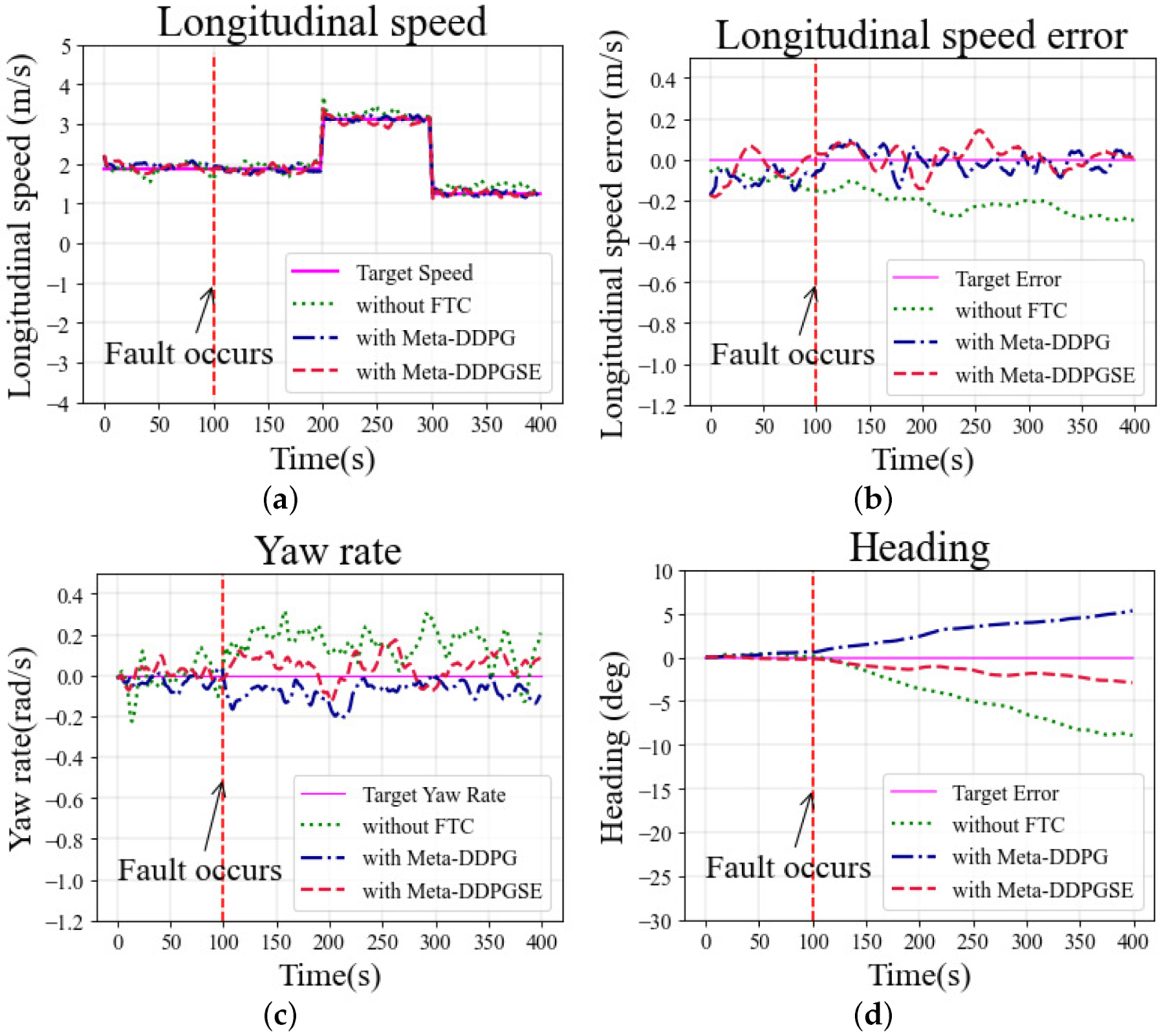
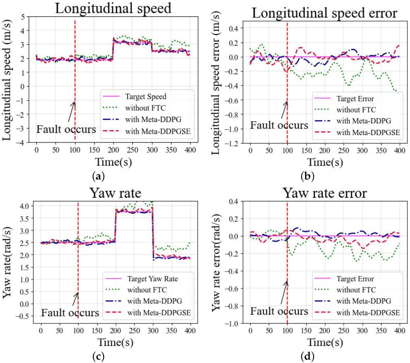
The longitudinal speed was set as 2.0 m/s at the beginning, 3.1 m/s at 200 s, and 1.2 m/s at 300 s, which was maintained until the end. The yaw rate was always 0 rad/s during the simulation in the straight scenario. The fault situation $F_1^{*}$ occurred at 100 s, and continued until the end of the simulation. The selected initial meta-trained model was fine-tuned for 200 steps to obtain a fine-tuned model, which was then used for vehicle control under fault situations.

The longitudinal speeds at different moments in the simulation are shown in Figure 7a. As observed in Figure 7b, the error in the case with the DDPG-based controller exceeded 0.2 m/s, significantly greater than in other cases. The yaw rates in different cases are shown in Figure 7c. The desired yaw rate was zero in the straight scenario. The cases with FTC methods maintained the yaw rate error within 0.2 rad/s; however, without FTC, the error exceeded 0.2 rad/s and fluctuated more drastically than in other cases. As shown in Figure 7d, the heading deviation was also larger in the case without FTC than other cases using FTC methods.

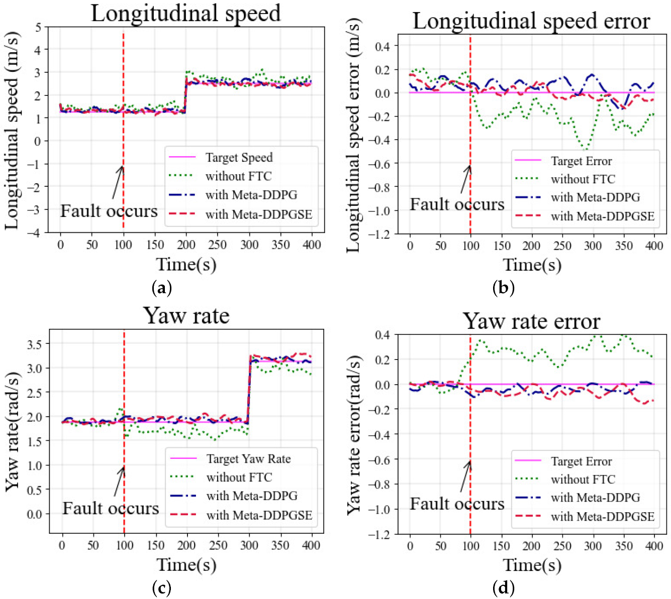
The second simulation in the straight scenario was conducted under fault situation $F_2^{*}$. The simulation results are shown in Figure 8, which had a similar trend to the simulation of fault situation $F_1^{*}$. Without FTC, the longitudinal speed error exceeded 0.2 m/s after the fault occurred, and the maximum error even reached 0.4 m/s, as shown in Figure 8a,b. The tracking performance showed no significant difference between cases with different FTC methods, and the errors in both cases were kept within 0.2 m/s, better than in the case without FTC. As observed in Figure 8c, the yaw rate errors in the cases with FTC methods were kept within 0.2 rad/s; however, without FTC, the maximum error exceeded 0.2 rad/s during the simulation. From Figure 8d, it can be observed that the heading deviation in the case without FTC exceeded 0.2 deg, which was greater than in other cases usingFTC methods. The above analysis indicates that both our proposed FTC method and the meta-DDPG-based FTC method worked well.

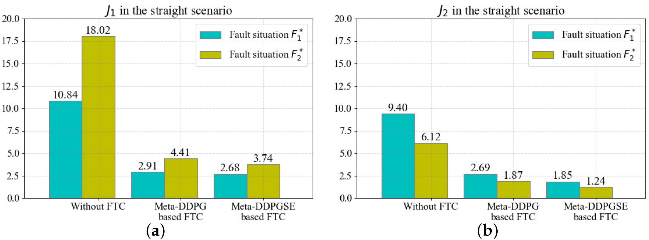
The above results show that fault situations severely affect the performance of desired value tracking, which can be overcome by the FTC methods. To illustrate the improvement when using our proposed FTC method more specifically, we quantitatively compared it with the meta-DDPG-based FTC method. Equation (24) was used to evaluate the desired value tracking performance. The quantitative evaluation results in the straight scenario are displayed in Figure 9.

The results for $J_1$ and $J_2$ in different cases were obtained based on the aforementioned simulations. The FTC method based on meta-DDPG reduced $J_1$ by $73.15\%$ in the fault situation $F_1^{*}$ and $75.53\%$ in the fault situation $F_2^{*}$, and reduced $J_2$ by $71.38\%$ in the fault situation $F_1^{*}$ and $69.44\%$ in the fault situation $F_2^{*}$. Similarly, the FTC method based on meta-DDPGSE reduced $J_1$ by $75.28\%$ in the fault situation $F_1^{*}$ and $79.25\%$ in the fault situation $F_2^{*}$, and reduced $J_2$ by $80.32\%$ in the fault situation $F_1^{*}$ and $79.74\%$ in the fault situation $F_2^{*}$. The quantitative evaluation results in the straight scenario demonstrate that both FTC methods can effectively reduce the severity of fault situations; however, the meta-DDPGSE-based FTC method performed better.

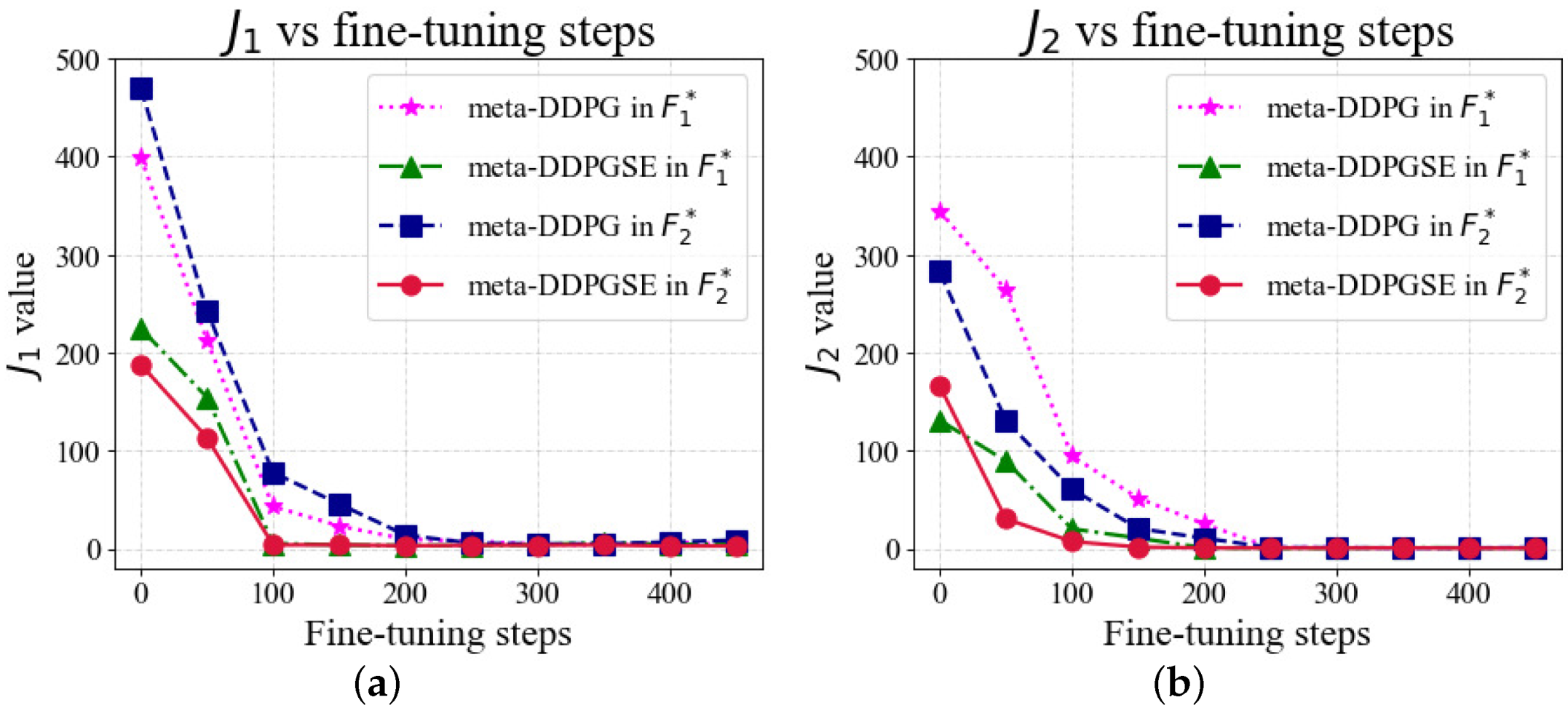
In the above simulations, the number of online fine-tuning steps of the meta-trained models was 200 in the different FTC methods. We also evaluated the online adaptation speed of different FTC methods through the effect of the online fine-tuning steps on the desired value tracking performance. In this simulation, vehicles were assigned the same desired values and fault situations $F_1^{*}$ and $F_2^{*}$ as in previous simulations, but we set different online fine-tuning steps. We analyzed $J_1$ and $J_2$ of the two FTC methods with numbers of different fine-tuning steps. When the number of fine-tuning steps was 0, the offline meta-trained model was directly used to control the vehicle after the fault occurred.

The simulation results are shown in Figure 10. Each data point in the figure is an average of the same process repeated five times. When the number of fine-tuning steps was 0, $J_1$ and $J_2$ obtained by the meta-DDPGSE-based FTC method were significantly smaller than those obtained by the meta-DDPG-based FTC method. This result indicates that the meta-DDPGSE-based FTC method can select a suitable meta-trained model for the current fault situation as the starting point of online adaptation. The meta-DDPGSE-based FTC method could achieve high performance after 100 steps of online fine-tuning, while the meta-DDPG-based FTC method needed 200 steps to achieve the same results, thus demonstrating that the meta-DDPGSE-based FTC method was able to adapt to fault situations more quickly than the meta-DDPG-based FTC method.

5.2. Simulations in the Cornering Scenario

Simulations of the cornering scenario were conducted to identify the vehicle’s cornering ability under fault situations. The fault situations assigned to the vehicle were consistent with those in Section 5.1 and are listed in Table 3. Figure 11 and Figure 12 show the simulation results of the vehicle under fault situations $F_1^{*}$ and $F_2^{*}$ in the cornering scenarios, respectively.

The longitudinal speed tracking results for the vehicle with fault situation $F_1^{*}$ in the cornering scenario are shown in Figure 11a,b. Without FTC, the longitudinal speed fluctuated sharply, and the maximum error exceeded 0.4 m/s, significantly worse than that in the cases using FTC methods. With FTC, the longitudinal speed tracking performance in the fault situation did not deteriorate significantly, and errors remained within 0.2 m/s. The yaw rate tracking results are shown in Figure 11c,d. After the fault situation $F_1^{*}$ occurred, the desired yaw rates were still well-tracked in the cases with FTC methods. However, without FTC, the yaw rate fluctuated sharply, and the error became significantly larger, which demonstrates that the case without FTC had no ability to track the desired yaw rate after the fault occurred.

Similar trends were observed in the simulation with fault situation $F_2^{*}$ in the cornering scenario, as shown in Figure 12. Without FTC, the longitudinal speed and yaw rate fluctuated more severely after fault situation $F_2^{*}$ occurred. The DDPG-based controller had no ability to track the desired value as accurately as before the fault situation $F_2^{*}$ occurred. With FTC, the tracking performance of the longitudinal speed and yaw rate was not significantly degraded, being similar to the tracking performance before the fault situation $F_2^{*}$ occurred. The longitudinal speed errors and yaw rate errors could be kept within 0.2 m/s and 0.2 rad/s, respectively. The results demonstrate that fault situations $F_1^{*}$ and $F_2^{*}$ can impose serious impacts on the desired value tracking performance; however, such impacts can be overcome by implementing FTC methods such as those based on meta-DDPG and meta-DDPGSE.

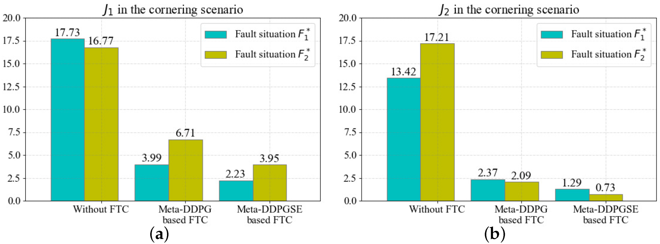
The results for $J_1$ and $J_2$ in the cornering scenario are shown in Figure 13. The FTC method based on meta-DDPG reduced $J_1$ by $77.50\%$ in the fault situation $F_1^{*}$ and $59.99\%$ in the fault situation $F_2^{*}$, and reduced $J_2$ by $82.34\%$ in the fault situation $F_1^{*}$ and $87.86\%$ in the fault situation $F_2^{*}$. Similarly, the FTC method based on meta-DDPGSE reduced $J_1$ by $87.42\%$ in the fault situation $F_1^{*}$ and $76.44\%$ in the fault situation $F_2^{*}$, and reduced $J_2$ by $90.39\%$ in the fault situation $F_1^{*}$ and $95.76\%$ in the fault situation $F_2^{*}$. The quantitative evaluations in the cornering scenario had the same results as in the straight scenario, indicating that the FTC methods can effectively improve the tracking performance of vehicles with faults.

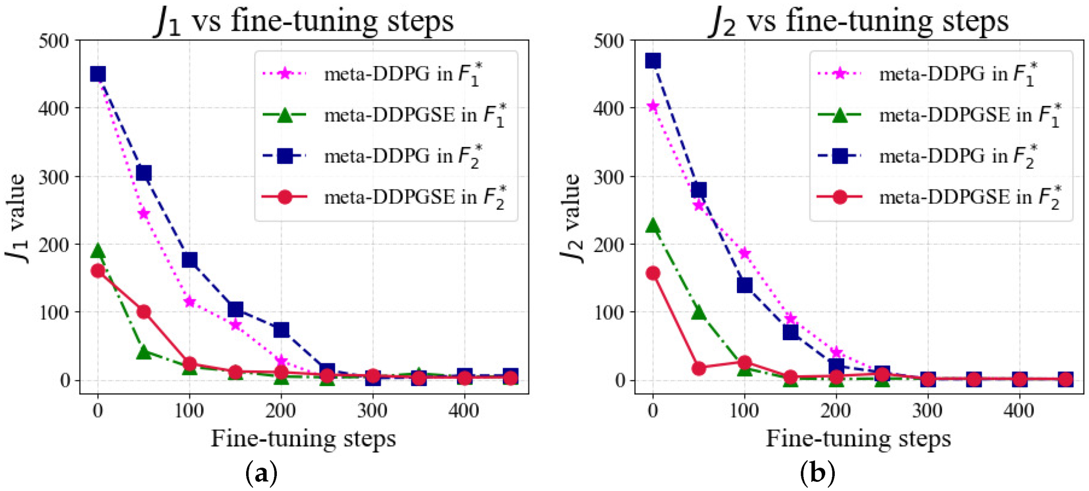
To better reflect the performance of our proposed FTC method, we set different numbers of online fine-tuning steps in the cornering scenario. The simulation results are shown in Figure 14. As the number of fine-tuning steps increased, $J_1$ and $J_2$ decreased with a similar trend as in the straight scenario. The meta-DDPGSE-based FTC method had the ability to select a suitable meta-trained model as the starting point for online adaptation, according to the current fault situation. The meta-DDPGSE-based FTC method could obtain good testing error results after 100 steps of online fine-tuning, while the meta-DDPG-based FTC method needed 200 steps to achieve the same results. Therefore, the proposed FTC method benefits from the selection of the most suitable initial meta-trained model, which makes it able to more quickly adapt to fault situations than the meta-DDPG-based FTC method.

6. Conclusions

In this work, we proposed a meta-DDPGSE-based FTC method for skid-steering vehicles, which could maintain the desired value tracking performance under different types of fault situations. Based on the DDPG algorithm, we developed an agent that can perform dual-channel control over the longitudinal speed and yaw rate of skid steering vehicles. Differing from conventional meta-RL methods, which only use a single meta-trained model for the entire task distribution, multiple initial meta-trained models were trained for different types of fault situations in the offline stage. We introduced the situation embedding model into the current meta-DDPG-based framework and developed a new FTC method based on meta-DDPGSE. Based on the online data set, the situation embedding model could select the most suitable initial meta-trained model as the starting point for adapting to the current fault situation. The simulation results from four testing scenarios demonstrated that, thanks to the selection of the most suitable meta-trained model, the meta-DDPGSE-based FTC method was able to more quickly adapt different types of fault situations, performing better than the considered baseline methods.

This work opens an exciting path for the FTC method of skid-steering vehicles using meta-RL methods under multiple types of fault situations. At present, we are exploring ways to extend this work by incorporating fault detection techniques. We also plan to apply the proposed FTC method to different vehicle systems, such as independent driving electric vehicles, as they are also prone to different types of fault situations.

References

1. Krecht, R.; Hajdu, C.; Ballagi, A. Possible Control Methods for Skid-Steer Mobile Robot Platforms. In Proceedings of the 2020 2nd IEEE International Conference on Gridding and Polytope Based Modelling and Control, Gyor, Hungary, 19–19 November 2020; pp. 31–34. [Google Scholar]
2. Liao, J.F.; Chen, Z.; Yao, B. Adaptive robust control of skid steer mobile robot with independent driving torque allocation. In Proceedings of the 2017 IEEE International Conference on Advanced Intelligent Mechatronics, Munich, Germany, 3–7 July 2017; pp. 340–345. [Google Scholar]
3. Fernandez, B.; Herrera, P.J.; Cerrada, J.A. A simplified optimal path following controller for an agricultural skid-steering robot. IEEE Access 2019, 7, 95932–95940. [Google Scholar] [CrossRef]
4. Zhang, Y.; Li, X.; Zhou, J.; Li, S.; Du, M. Hierarchical control strategy design for a 6WD unmanned skid-steering vehicle. In Proceedings of the 2018 IEEE International Conference on Mechatronics and Automation, Changchun, China, 5–8 August 2018; pp. 2036–2041. [Google Scholar]
5. Zhang, H.; Yang, X.; Liang, J.; Xu, X.; Sun, X. GPS Path Tracking Control of Military Unmanned Vehicle Based on Preview Variable Universe Fuzzy Sliding Mode Control. Machines 2021, 12, 304. [Google Scholar] [CrossRef]
6. Zhang, X.; Xie, Y.; Jiang, L.; Li, G.; Meng, J.; Huang, Y. Fault-Tolerant Dynamic Control of a Four-Wheel Redundantly-Actuated Mobile Robot. IEEE Access 2019, 7, 157909–157921. [Google Scholar] [CrossRef]
7. Hua, C.; Li, L.; Ding, S.X. Reinforcement Learning-aided Performance-driven Fault-tolerant Control of Feedback Control Systems. IEEE Trans. Autom. Control. 2021, 99, 1. [Google Scholar] [CrossRef]
8. Antonio, P.; Lorenzo, R.C. Discrete-Time selfish Routing Converging to the Wardrop Equilibrium. IEEE Trans. Autom. Control. 2019, 64, 1288–1294. [Google Scholar]
9. Stolte, T. Actuator Fault-Tolerant Vehicle Motion Control: A Survey. arXiv 2021, arXiv:2103.13671. [Google Scholar]
10. Ruder, S. An Overview of Multi-Task Learning in Deep Neural Networks. arXiv 2017, arXiv:1706.05098. [Google Scholar]
11. Ma, J.Q.; Zhao, Z.; Yi, X.Y.; Chen, J.L.; Hong, L.C.; Chi, E.H. Modeling task relationships in multi-task learning with multi-gate mixture-of-experts. In Proceedings of the 24th ACM International Conference on Knowledge Discovery & Data Mining, London, UK, 19–23 August 2018; pp. 1930–1939. [Google Scholar]
12. Finn, C.; Abbeel, P.; Levine, S. Model-Agnostic Meta-Learning for Fast Adaptation of Deep Network. In Proceedings of the 34th International Conference on Machine Learning, Sydney, Australia, 6–11 August 2017; Volume 70, pp. 1126–1135. [Google Scholar]
13. Ahmed, I.; Quiones, G.M.; Biswas, G. Complementary Meta-Reinforcement Learning for Fault-Adaptive Control. arXiv 2020, arXiv:2009.12634. [Google Scholar] [CrossRef]
14. Ahmed, I.; Khorasgani, H.; Biswas, G. Comparison of Model Predictive and Reinforcement Learning Methods for Fault Tolerant Control. arXiv 2020, arXiv:2008.04403. [Google Scholar] [CrossRef]
15. Ahmed, I.; Quiones, G.M.; Biswas, G. Fault-Tolerant Control of Degrading Systems with On-Policy Reinforcement Learning. arXiv 2020, arXiv:2008.04407. [Google Scholar] [CrossRef]
16. Ahmed, I.; Quiones, G.M.; Biswas, G. Performance-Weighed Policy Sampling for Meta-Reinforcement Learning. arXiv 2020, arXiv:2012.06016. [Google Scholar]
17. Yel, E.; Bezzo, N. A Meta-Learning-Based Trajectory Tracking Framework for UAVs under Degraded Conditions. arXiv 2021, arXiv:2104.15081. [Google Scholar]
18. Liang, C.; Wang, W.; Liu, Z.; Lai, C.; Zhou, B. Learning to Guide: Guide Law Based on Deep Meta-learning and Model Predictive Path Integral Control. IEEE Access 2019, 7, 47353–47365. [Google Scholar] [CrossRef]
19. Zhao, F.; You, K.; Fan, Y.; Yan, G. Velocity Regulation for Automatic Train Operation via Meta-Reinforcement Learning. In Proceedings of the 2020 39th Chinese Control Conference, Shenyang, China, 27–30 July 2020; pp. 1969–1974. [Google Scholar]
20. Li, B.; Gan, Z.; Chen, D.; Aleksandrovich, D. UAV Maneuvering Target Tracking in Uncertain Environments Based on Deep Reinforcement Learning and Meta-Learning. Remote Sens. 2020, 12, 3789. [Google Scholar] [CrossRef]
21. Ma, Y.; Zhao, S.L.; Wang, W.X.; Li, Y.M.; King, I. Multimodality in meta-learning: A comprehensive survey. arXiv 2021, arXiv:2109.13576. [Google Scholar]
22. Yu, T.H.; Quillen, D.; He, Z.P.; Julian, R.; Hausman, K.; Finn, C.; Levine, S. Meta-World: A Benchmark and Evaluation for Multi-Task and Meta Reinforcement Learning. In Proceedings of the Conference on Robot Learning, Cambridge, MA, USA, 16–18 November 2020; Volume 100, pp. 1094–1100. [Google Scholar]
23. Risto, V.; Sun, S.H.; Hu, H.X.; Lim, J.J. Multimodal model-agnostic meta-learning via task-aware modulation. arXiv 2019, arXiv:1910.13616. [Google Scholar]
24. Risto, V.; Sun, S.H.; Hu, H.X.; Lim, J.J. Model-Agnostic Meta-Learning for Multimodal Task Distributions. In Proceedings of the ICLR 2019 Conference, New Orleans, LA, USA, 6–9 May 2019. [Google Scholar]
25. Lin, L.; Li, Z.G.; Guan, X.H.; Wang, P.H. Meta Reinforcement Learning with Task Embedding and Shared Policy. arXiv 2019, arXiv:1905.06527. [Google Scholar]
26. Achille, A.; Lam, M.; Tewari, R.; Ravichandram, A.; Maji, S.; Fowlkes, C.C.; Soatto, S.; Perona, P. TASK2Vec: Task embedding for meta-learning. In Proceedings of the IEEE/CVF International Conference on Computer Visio, Seoul, Korea, 27–28 October 2019; pp. 6430–6439. [Google Scholar]
27. Chen, X.H.; Tang, S.Y.; Muandet, K. MATE: Plugging in model awareness to task embedding for meta-learning. Nerual Inf. Process. Syst. 2020, 33, 11865–11877. [Google Scholar]
28. Kaushik, R.; Anne, T.; Mount, J.B. Fast Online Adaptation in Robotics through Meta-Learning Embeddings of Simulated Priors. In Proceedings of the 2020 IEEE/RSJ International Conference on Intelligent Robots and Systems, Las Vegas, NV, USA, 24–30 October 2020; pp. 5269–5276. [Google Scholar]
29. Jin, L.; Tian, D.; Zhang, Q.; Wang, J. Optimal Torque Distribution Control of Multi-Axle Electric Vehicles with In-wheel Motors Based on DDPG Algorithm. Energies 2020, 13, 1331. [Google Scholar] [CrossRef] [Green Version]
30. Hu, H.Y.; Lu, Z.Y.; Wang, Q.; Zheng, C.Y. End-to-End Automated Lane-Change Maneuvering Considering Driving Style Using a Deep Deterministic Policy Gradient Algorithm. Sensors 2020, 20, 5443. [Google Scholar] [CrossRef]
31. Yu, L.L.; Shao, X.Y.; Wei, Y.D.; Zhou, K.J. Intelligent Land-Vehicle Model Transfer Trajectory Planning Method Based on Deep Reinforcement Learning. Sensors 2018, 18, 2905. [Google Scholar]
32. Sun, Y.; Zhang, C.; Zhang, G.; Xu, H.; Ran, X. Three-Dimensional Path Tracking Control of Autonomous Underwater Vehicle Based on Deep Reinforcement Learning. J. Mar. Sci. Eng. 2019, 7, 443. [Google Scholar] [CrossRef] [Green Version]
33. Sliver, D.; Lever, G.; Heess, N.; Degris, T.; Wierstra, D.; Riedmiller, M. Deterministic policy gradient algorithms. In Proceedings of the 31st International Conference on Machine Learning, Beijing, China, 21–26 June 2014; Volume 32, pp. 387–395. [Google Scholar]
34. Lillicrap, T.P.; Hunt, J.J.; Pritzel, A.; Heess, N.; Erez, T.; Tassa, Y.; Silver, D.; Wierstra, D. Continuous control with deep reinforcement learning. arXiv 2015, arXiv:1509.02971. [Google Scholar]
35. Mnih, V.; Kavukcuoglu, K.; Silver, D.; Graves, A.; Antonoglo, I.; Wierstra, D.; Riedmiller, M. Playing Atari with Deep Reinforcement Learning. arXiv 2013, arXiv:1312.5602. [Google Scholar]
36. Dai, H.T.; Chen, P.Z.; Y, H. Metalearning-Based Fault-Tolerant Control for Skid Steering Vehicles under Actuator Fault Conditions. Sensors 2022, 22, 845. [Google Scholar] [CrossRef]
37. Liao, J.F.; Chen, Z.; Yao, B. Performance-Oriented Coordinated Adaptive Robust Control for Four-wheel Independently Driven Skid Steer Mobile Robot. IEEE Access 2017, 5, 19048–19057. [Google Scholar] [CrossRef]
38. Liao, J.; Chen, Z.; Yao, B. Model-Based Coordinated Control of Four-Wheel Independently Driven Skid Steer Mobile Robot with Wheel-Ground Interaction and Wheel Dynamics. IEEE Trans. Ind. Inform. 2019, 15, 1742–1752. [Google Scholar] [CrossRef]
39. Zhang, B.H.; Lu, S.B. Fault-tolerant control for four-wheel independent actuated electric vehicle using feedback linearization and cooperative game theory. Control. Eng. Pract. 2020, 101, 104510. [Google Scholar] [CrossRef]
40. Zhang, H.; Zhao, W.; Wang, J. Fault-Tolerant Control for Electric Vehicles with Independently Driven in-Wheel Motors Considering Individual Driver Steering Characteristics. IEEE Trans. Veh. Technol. 2019, 68, 4527–4536. [Google Scholar] [CrossRef]
Figure 1. Skid-steering vehicle diagram.
Actuators 11 00072 g001
Figure 2. Flowchart of the meta-DDPGSE-based FTC method.
Actuators 11 00072 g002
Figure 3. Framework of the meta-DDPGSE-based FTC method: (a) Offline stage; and (b) Online stage.
Actuators 11 00072 g003
Figure 4. The structures of policy neural networks (a) and Q-value neural networks (b).
Actuators 11 00072 g004
Figure 5. The structure of situation embedding networks.
Actuators 11 00072 g005
Figure 6. The total reward trends in the meta-testing.
Actuators 11 00072 g006
Figure 7. Simulation results in the straight scenario with fault F 1 * : (a) Longitudinal speed; (b) Longitudinal speed error; (c) Yaw rate; (d) Heading.
Actuators 11 00072 g007
Figure 8. Simulation results in the straight scenario with fault F 2 * : (a) Longitudinal speed; (b) Longitudinal speed error; (c) Yaw rate; (d) Heading.
Actuators 11 00072 g008
Figure 9. The quantitative evaluation in the straight scenario: (a) J 1 in the straight scenario; (b) J 2 in the straight scenario.
Actuators 11 00072 g009
Figure 10. Effect of number of fine-tuning steps on J 1 and J 2 in the straight scenario: (a) J 1 value vs. fine-tuning steps; (b) J 2 value vs. fine-tuning steps.
Actuators 11 00072 g010
Figure 11. Simulation results in the cornering scenario with fault F 1 * : (a) Longitudinal speed; (b) Longitudinal speed error; (c) Yaw rate; (d) Yaw rate error.
Actuators 11 00072 g011
Figure 12. Simulation results in the cornering scenario with fault F 2 * : (a) Longitudinal speed; (b) Longitudinal speed error; (c) Yaw rate; (d) Yaw rate error.
Actuators 11 00072 g012
Figure 13. The quantitative evaluation in the cornering scenario: (a) J 1 in the cornering scenario; (b) J 2 in the cornering scenario.
Actuators 11 00072 g013
Figure 14. Effect of fine-tuning steps on J 1 and J 2 in the cornering scenario: (a) J 1 value vs. fine-tuning steps; (b) J 2 value vs. fine-tuning steps.
Actuators 11 00072 g014