Article

H-Infinity Observer for Vehicle Steering System with Uncertain Parameters and Actuator Fault

School of Control Engineering, Northeastern University at Qinhuangdao, Qinhuangdao 066004, China
*
Author to whom correspondence should be addressed.
Actuators 2022, 11(2), 43; https://doi.org/10.3390/act11020043
Submission received: 13 December 2021 / Revised: 11 January 2022 / Accepted: 26 January 2022 / Published: 28 January 2022

Abstract

:
In this paper, an actuator fault diagnosis and reconfiguration problem is discussed for an uncertain vehicle steering system with external disturbances. Aiming at the factors affecting the control performance, a fault reconstruction strategy based on H-infinity observer is designed to improve the vehicle stability under complex conditions when the actuator fails. Firstly, aiming at the uncertain part caused by the road condition transformation, a mathematical model of dual input and dual output four-wheel steering system is established. Secondly, an augmented system is constructed in which the augmented state vector consists of the original state and actuator faults. Thirdly, the H-infinity observer is designed, and the gain of the observer is obtained by the Lyapunov function and linear matrix inequality. Finally, the effectiveness of the proposed strategy is verified by MATLAB/Simulink and Carsim co-simulation.

1. Introduction

With the increase in the number of vehicles on the road, the frequency of traffic accidents is also gradually increasing [1]. According to investigation and analysis, many accidents are caused by the fault of the vehicle’s steering system. The steering system can directly affect the driver’s driving experience and improve the safe driving of the vehicle. The steer-by-wire (SbW) system is an electronically controlled vehicle system and can greatly improve the dynamic performance of vehicle [2,3], but actuator fault often occurs in the vehicle steering system due to (age) long period, high load and high strength, which affects the normal operation of equipment and even causes safety accidents. The SbW system is sensitive to various types of faults caused by the component and needs higher fault diagnosis and fault tolerance. Thus, research on the actuator fault diagnosis of vehicle steering systems is of great significance to reduce the probability of traffic accidents.
The common actuator fault types of the vehicle steering system include lock-in-place fault, permanent fault, periodic fault and fluctuating actuator fault [4]. The lock-in-place failure corresponds to the situation when the front wheel angle is stuck for a period of time [5]. The expansion or contraction of the wire connectors may cause permanent actuator fault. The continuous vibration of the vehicle may lead to actuator periodic fault [6]. The fluctuating actuator faults are caused by electromagnetic interference, radiation, temperature changes or motor driver-related faults. When actuator fault occurs, the vehicle will lose driving stability and driving safety. Researchers have been focusing on fault detection (FD), fault diagnosis and isolation (FDI) and fault-tolerant control (FTC) for many years and have put forward many practical fault diagnosis methods [7,8]. Generally, fault diagnosis strategies are divided based on their diagnosis method: the analytic model-based method diagnoses faults according to the system model and residual error; the signal processing method diagnoses faults by analyzing the symbolic characteristics of system signals; and the knowledge-based method diagnoses faults through mass data simulation training [9]. For model-based approaches, the actual system is modeled by physical principles or system identification methods. Residuals are generated by comparing the measured output of the real system with the model. The state observer-based approach is the representative of model-based diagnosis. In [10], online fault detection and isolation of multiple faults of hybrid power system based on model diagnosis architecture is proposed. For the signal-based approach, the diagnostic process is based on real-time assessment of symptoms obtained through feature extraction. Authors of [11] propose a new fault diagnosis method based on parameter identification. The data-driven approach is based on extracting mapping knowledge from the fault database, which can be obtained from historical data and online monitoring data. An intelligent time-adaptive data-driven fault diagnosis scheme is studied in [12]. The signal-based methods are often slow in diagnosis and highly sensitive to system load conditions. The data-driven methods are not ideal in diagnosis speed and accuracy and are heavy in training and tuning. In general, most actuator fault diagnosis methods are model-based because of their high speed and load independence. In recent years, scholars have paid extensive attention to actuator faults of control systems and obtained abundant research results in the direction of unmanned surface vessel [13], wind turbine [14], hypersonic aircraft [15], electric scooter [16] and so on. At the same time, many scholars have conducted pure theoretical studies on actuator faults [17,18].
To improve the reliability of vehicles, the actuator fault of the vehicle steering system is studied. For the vehicle system, the observer is designed based on the actuator fault extended system model in [19]. A fault observer is proposed to estimate the fault information of the SbW vehicle system with actuator faults, system uncertainties and disturbances [4]. A robust control algorithm based on output feedback is proposed for the vehicle steering control system with actuator fault and the uncertainties in the tire cornering stiffness [20]. A robust pole assignment yaw controller with parametric uncertainties verifies the flexibility of vehicles [21]. Furthermore, the research object is a front-wheel steering system. To improve the vehicle maneuverability at low speeds and enhance the vehicle stability at high speeds, four-wheel steering (4WS) vehicles have been studied. The 4WS adds rear-wheel steering system on the basis of front-wheel steering to realize active or follow-up steering function of the rear wheels following the front wheels during driving. When the vehicle is traveling at low speeds, the front and rear wheels turn backward, which can reduce the turning radius of the vehicle and accelerate the response speed of the vehicle. When driving at high speeds, the front and rear wheels rotate in the same direction, which can improve the stability of the vehicle. More and more automobile enterprises have begun to research and apply 4WS technology to vehicles. For example, Nissan, Toyota, Ford and General Motors have developed four-wheel steering technology very rapidly. With the application of SbW and 4WS, manufacturers can improve the stability and driving flexibility of the vehicle. Some scholars have conducted in-depth research on the 4WS system. In view of the uncertainties in the 4WS system model, the optimized control strategy is designed to improve vehicle handling [22]. Authors of [23] consider the existence of external interference in the SbW system and adopt the method of combining feedforward control and feedback control to improve the handling stability of the 4WS system. The authors of [24] propose a coordinated control method of 4WS system and electronic stability program based on road adhesion coefficient to improve vehicle stability under extreme conditions. Authors of [25] consider external interference and the uncertainty of tire sidetrack stiffness and propose an observation-based control strategy to improve the maneuverability and stability of four-wheel independent-drive electric vehicles with an active front-wheel steering system. Considering the occurrence of actuator faults, the state estimator is designed by considering rear-wheel steering in [26], but uncertain factors in the system are not considered. Actuator faults and uncertain factors are considered for 4WS vehicles in [27], obtaining some results, but the effect of non-linear external disturbance on actual system performance is not studied.
In view of the above problems, considering the uncertainty factors and actuator faults in the 4WS system with external disturbance, an H-infinity observer-based fault diagnosis algorithm was designed. To make the research more convenient and realize the feasibility of the control strategy, the research object of this paper was a simplified vehicle model, which can meet the basic dynamic analysis condition. Considering the uncertainty caused by the road surface, closer to the actual vehicle, a robust H-infinite observer was designed based on the Lyapunov method and LMI technology, and theoretical proof was constructed. The effectiveness of the designed observer was verified by MATLAB/ Simulink and Carsim co-simulation under complex driving conditions.
The rest of this article is organized as follows: Section 2 briefly presents the vehicle model of 4WS system. In Section 3, an actuator fault diagnosis observer is designed. In Section 4, the proposed H-infinity observer is simulated and verified. Finally, Section 5 draws some conclusions and further perspectives.

2. System Modeling and Problem Formulation

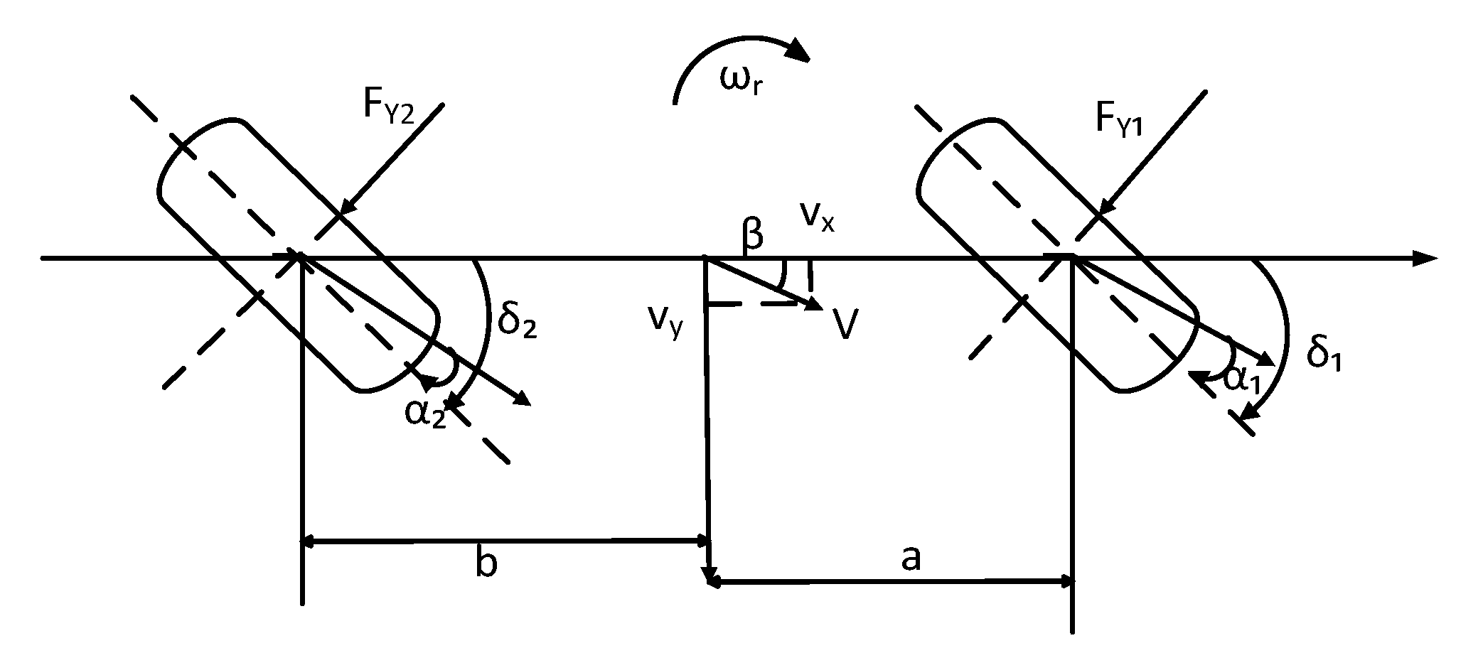
The establishment of a mathematical model is of great significance to the design of the control system, and the mathematical model for the whole vehicle is very complex. The vehicle system has strong non-linear and uncertain characteristics, so it is difficult to describe an accurate vehicle dynamics model. To make the problem easy to analyze, some assumptions are made when establishing the mathematical model, and the vehicle system is simplified to a two-degree-of-freedom model so that it is easier to design the control strategy. The two-degree-of-freedom model contains the yaw rate and side slip angle parameters that describe the vehicle handling stability and can reflect the most basic characteristics of the required curve motion [28]. The two-degree-of-freedom model quantitatively describes the key parameters that affect the lateral motion of vehicle, such as the position of vehicle centroid and the tire side deflection characteristics, which is the basis for the study of vehicle operating stability. Many theories and experiments have proved that the two-degree-of-freedom of a four-wheel steering vehicle model can reflect the actual physical process of the vehicle. Therefore, a two-DOF vehicle dynamics model was established. The model as the ideal steering characteristics was used to study the vehicle stability in our research, as shown in Figure 1.
The major parameters are given as follows: F Y 1 and F Y 2 are the lateral forces of the front and rear wheels, respectively; δ 1 and δ 2 are the front and rear steering angle, respectively; α 1 and α 2 are the side angles of the front and rear wheels, respectively; ω r is the yaw rate of the vehicle; β is the side slip angle of the vehicle; v x is the longitudinal speed of the vehicle; v y is the lateral speed of the vehicle; I z is the yaw moment of inertia around the center of mass; a and b are the distances from the center of gravity to the front and rear axles, respectively.
In this study, the dynamic equations are given based on the force analysis of the two-degree-of-freedom vehicle model [29].
{ F Y = F Y 1 cos δ 1 + F Y 2 M Z = a F Y 1 cos δ 1 b F Y 2
where Σ F Y and Σ M z are the resultant forces of the vehicle in the y-axis direction and the sum of the moments around the center of mass, respectively.
Based on Newton’s second law and the moment of inertia, Equation (1) is rewritten as:
{ m a Y = F Y 1 cos δ 1 + F Y 2 I Z ω ˙ r = a F Y 1 cos δ 1 b F Y 2
where m is the vehicle mass, and a y is the lateral acceleration of vehicle.
The lateral acceleration at the mass center can be written as:
a y = v ˙ + u ω r
When the road condition of the vehicle changes or when the road adhesion coefficient changes or reaches the range of non-linear tire, the lateral stiffness of the tire will change to some extent, resulting in uncertainty and affecting the vehicle steering [25].
At this point, there is a non-linear relationship between tire side force and tire side angle, and the tire side deflection characteristics can be expressed as:
{ F Y 1 = ( k 1 + σ N k 1 ) α 1 F Y 2 = ( k 2 + σ N k 2 ) α 2
where k 1 and k 2 are the lateral stiffness values of the front and rear wheels, respectively. N represents the deviation from the lateral stiffness amplitude. σ is time-dependent, and σ 1 is satisfied.
The relationship between the side slip angle and the angle of the wheel can be obtained, as we know the geometric relationship.
{ α 1 = β + a ω r v x δ 1 α 2 = β b ω r v x δ 2
The δ 1 , δ 2 and β are generally small when the vehicle is traveling, so we have:
cos δ 1 1
cos δ 2 1
β tan β = v y v x
β ˙ = v ˙ u
Substituting Equations (3)–(9) into Equation (2), we have:
{ ω ˙ r = a 2 k 1 + b 2 k 2 v x I z ω r + a 2 σ N k 1 + b 2 σ N k 2 v x I z ω r + a k 1 b k 2 I z β + a σ N k 1 b σ N k 2 I z β a k 1 I z δ 1 a σ N k 1 I z δ 1 + b k 2 I z δ 2 + b σ N k 2 I z δ 2 β ˙ = ( a k 1 b k 2 m v x 2 1 ) ω r + a σ N k 1 b σ N k 2 m v x 2 ω r + k 1 + k 2 m v x β + σ N k 1 + σ N k 2 m v x β k 1 m v x δ 1 σ N k 1 m v x δ 1 k 2 m v x δ 2 σ N k 2 m v x δ 2
The state-space equation of the vehicle model is obtained as follows:
{ x ˙ ( t ) = ( A + Δ A ) x ( t ) + ( B + Δ B ) u ( t ) y ( t ) = C x ( t )
where x ( t ) = [ ω r β ] T is the system state vector, and u ( t ) = [ δ 1 δ 2 ] T is the system input vector. The matrices satisfy the following form:
A = [ a 2 k 1 + b 2 k 2 v x I z a k 1 b k 2 I z a k 1 b k 2 m v x 2 1 k 1 + k 2 m v x ] ,   Δ A = [ a 2 σ N k 1 + b 2 σ N k 2 v x I z a σ N k 1 b σ N k 2 I z a σ N k 1 b σ N k 2 m v x 2 σ N k 1 + σ N k 2 m v x ] = D 1 F E 1 ,   B = [ a k 1 I z b k 2 I z k 1 m v x k 2 m v x ] ,   Δ B = [ a σ N k 1 I z b σ N k 2 I z σ N k 1 m v x σ N k 2 m v x ] = D 2 F E 2 ,   F = [ σ 0 0 σ ] ,   F I ,   D 1 = [ a 2 N k 1 + b 2 N k 2 v x I z a N k 1 b N k 2 I z a N k 1 b N k 2 m v x 2 N k 1 + N k 2 m v x ] ,   E 1 = [ 1 0 0 1 ] = E 2 ,   D 2 = [ a N k 1 I z b N k 2 I z N k 1 m v x N k 2 m v x ] ,   C = [ 1 0 0 1 ]
After a long period of operation, actuator fault will inevitably occur. During the actual operation, the hardware may be suddenly damaged, resulting in sudden fault. With the change of time and environment, the component parameters change slowly and cause slow fault. The components of the vehicle aging and poor contact produce intermittent faults.
The fault of the steering system may not only cause steering difficulties but may even cause serious traffic accidents when the steering is not timely, affecting personal safety, and the actuator fault of the steering system can act as the system inputs [27]. Considering the fault of the steering system, the state equation can be expressed by in the following form [29]:
{ x ˙ ( t ) = ( A + Δ A ) x ( t ) + ( B + Δ B ) u ( t ) + ( B + Δ B ) f a y ( t ) = C x ( t )
where f a = [ f a f f a r ] T denotes actuator fault.
In the actual control system of vehicle, establishing a high-precision vehicle model is a key factor for actuator fault diagnosis. The vehicle system is a highly non-linear complex system, and there are often various non-linear factors in the modeling process. At the same time, there will be some external disturbances in the actual driving. The disturbances mainly come from load changes, parameter disturbances, crosswind, tire rolling resistance and other unmodeled items, which are mismatched disturbances and cannot be completely eliminated [30]. Combined with the above factors, the system model is given as follows:
{ x ˙ ( t ) = ( A + Δ A ) x ( t ) + ( B + Δ B ) u ( t ) + ( B + Δ B ) f a + G ˜ d ( t ) + φ ˜ ( x ) y ( t ) = C x ( t )
where d ( t ) represents the external road disturbance caused by slope, crosswind, road type, etc.; G ˜ represents the corresponding coefficient matrix; and φ ˜ ( x ) represents the non-linear disturbance.
By taking the fault as an additional state variable, an uncertain system model related to the actuator fault can be constructed as:
{ [ x ˙ ( t ) f ˙ a ] = [ A B 0 0 ] [ x ( t ) f a ] + [ B 0 ] u ( t ) + [ Δ A Δ B 0 0 ] [ x ( t ) f a ] + [ Δ B 0 ] u ( t ) + [ G ˜ 0 ] d ( t ) + [ φ ˜ ( x ) 0 ] z ( t ) = [ C 0 0 I ] [ x ( t ) f a ]
The augmented system is constructed as the following extended state-space model:
{ x ¯ ˙ ( t ) = A ¯ x ¯ ( t ) + B ¯ u ( t ) + Δ A ¯ x ¯ ( t ) + Δ B ¯ u ( t ) + G d + φ ( x ) z ( t ) = C ¯ x ¯ ( t )
where x ¯ ( t ) = [ x ( t ) f a ] , A ¯ = [ A B 0 0 ] , Δ A ¯ = [ Δ A Δ B 0 0 ] = D ¯ 1 F E ¯ 1 , B ¯ = [ B 0 ] , Δ B ¯ = [ Δ B 0 ] = D ¯ 2 F E 2 , C ¯ = [ C 0 0 I ] , D ¯ 1 = [ D 1 0 ] , D ¯ 2 = [ D 2 0 ] , E ¯ 1 = [ E 1 0 ] , G = [ G ˜ 0 ] , φ ( x ) = [ φ ˜ ( x ) 0 ] .

3. Design of H-Infinity Observer

For the reconstructed system (15), the H-infinite observer is designed considering the existence of parameter uncertainties and external disturbances. The designed controller can ensure the robustness and improve the accuracy of fault judgment. According to the Lyapunov method and LMI technology, it is proved that the proposed strategy can make the system asymptotically stable and achieve H-infinite performance index.
When the controlled object has the following indicators:
(1)
When interference d = 0 , the closed-loop system is asymptotically stable; and
(1)
For any d [ 0 , ] , the controlled output z ( t ) meets the H performance constraint z ( t ) λ d ,
the observer and controller satisfying the above conditions exist, and the system is said to be robustly stabilized with λ norm bound H under the action of the controller.
Assumption 1.
[31] The non-linear function φ ˜ ( x ) in system (13) satisfies the following Lipschitz condition:
φ ˜ ( x 2 ) φ ˜ ( x 1 ) ε x 2 x 1
where ε > 0 is called the Lipschitz constant, and φ ˜ ( 0 ) = 0 .
The following lemma is used to design an expected robust observer for the uncertain system (15):
Lemma 1.
[32] For any vector x , y with appropriate dimensions and positive scalar α , the following inequality holds:
± 2 x T y α x T x + α 1 y T y
Lemma 2.
[32] If Z = [ Z 11 Z 12 Z 21 Z 22 ] is a symmetric matrix, then the following three conditions are equivalent:
( 1 ) Z < 0 ; ( 2 ) Z 11 < 0 , Z 22 Z 12 T Z 11 1 Z 12 < 0 ; ( 3 ) Z 22 < 0 , Z 11 Z 12 Z 22 1 Z 12 T < 0 ;
For the augmented system (15), the state observer is designed as follows.
{ x ¯ ^ ˙ ( t ) = A ¯ x ¯ ^ ( t ) + B ¯ u ( t ) + L ( z ( t ) z ^ ( t ) ) + φ ( x ^ ) z ^ ( t ) = C ¯ x ¯ ^ ( t )
where x ¯ ^ ( t ) , z ^ ( t ) are the estimate of system state x ¯ ( t ) and output z ( t ) , respectively, and L is the gain matrix of the observer.
Let e ( t ) denotes the state estimation error, e y ( t ) denote the output estimation error and e f ( t ) denote the fault estimation error. The system state error is defined as:
e ( t ) = x ¯ ( t ) x ¯ ^ ( t )
e y ( t ) = z ( t ) z ^ ( t )
e f ( t ) = φ ( x ) φ ( x ^ )
The dynamic equation of state estimation error can be expressed as follows:
e ˙ ( t ) = x ¯ ˙ ( t ) x ¯ ^ ˙ ( t )   = A ¯ x ¯ ( t ) + B ¯ u ( t ) + Δ A ¯ x ¯ ( t ) + Δ B ¯ u ( t ) + G d + φ ( x ) ( A ¯ x ¯ ^ ( t ) + B ¯ u ( t ) + L ( y ( t ) y ^ ( t ) ) + φ ( x ^ ) )   = ( A ¯ L C ¯ ) e ( t ) + Δ A ¯ x ¯ ( t ) + Δ B ¯ u ( t ) + G d + e f ( t )
The observer-based state feedback controller is given by:
u ( t ) = M x ¯ ^ ( t )
where M is the feedback gain matrix.
Then from Equations (15) and (18)–(23), we have:
x ¯ ˙ ( t ) = A ¯ x ¯ ( t ) + B ¯ u ( t ) + Δ A ¯ x ¯ ( t ) + Δ B ¯ u ( t ) + G d + φ ( x ) = A ¯ x ¯ ( t ) + Δ A ¯ x ¯ ( t ) B ¯ M x ¯ ^ ( t ) Δ B ¯ M x ¯ ^ ( t ) + G d + φ ( x ) = ( A ¯ + Δ A ¯ ( B ¯ M + Δ B ¯ M ) ) x ¯ ( t ) + ( B ¯ M + Δ B ¯ M ) e ( t ) + G d + φ ( x )
e ˙ ( t ) = x ¯ ˙ ( t ) x ¯ ^ ˙ ( t ) = ( A ¯ L C ¯ ) e ( t ) + Δ A ¯ x ¯ ( t ) Δ B ¯ M x ¯ ^ ( t ) + G d + e f ( t ) = ( A ¯ L C ¯ + Δ B ¯ M ) e ( t ) + ( Δ A ¯ Δ B ¯ M ) x ¯ ( t ) + G d + e f ( t )
Theorem 1.
Given a positive scalar α and γ , the controller gain is selected as M = γ B ¯ T Q , if there exist positive-definite symmetric matrix P, Q and matrix X to satisfy that Equations (26) and (27), shown in a form as follows:
[ Ω 1 P Q T B ¯ E ¯ 2 T P D ¯ 2 P D ¯ 1 P D ¯ 2 Q T B ¯ E ¯ 2 T Q T B ¯ P G P 1 α 1 1 I 0 0 0 0 0 0 0 E ¯ 2 B ¯ T Q 0 1 α 2 γ I 0 0 0 0 0 0 D ¯ 2 T P 0 0 1 α 2 1 γ I 0 0 0 0 0 D ¯ 1 T P 0 0 0 1 α 3 1 I 0 0 0 0 D ¯ 2 T P 0 0 0 0 1 α 4 1 γ I 0 0 0 E ¯ 2 B ¯ T Q 0 0 0 0 0 1 α 8 γ I 0 0 B ¯ T Q 0 0 0 0 0 0 1 α 9 γ I 0 G T P 0 0 0 0 0 0 0 1 2 λ 2 I ] < 0
[ Ω 2 Q T B ¯ Q T B ¯ E ¯ 2 T Q Q D ¯ 1 Q T B ¯ E ¯ 2 T Q D ¯ 2 Q D ¯ 2 Q B ¯ Q G B ¯ T Q 1 2 γ I 0 0 0 0 0 0 0 0 E ¯ 2 B ¯ T Q 0 1 α 4 γ I 0 0 0 0 0 0 0 Q 0 0 1 α 5 1 I 0 0 0 0 0 0 D ¯ 1 T Q 0 0 0 1 α 6 1 I 0 0 0 0 0 E ¯ 2 B ¯ T Q 0 0 0 0 1 α 7 γ I 0 0 0 0 D ¯ 2 T Q 0 0 0 0 0 1 α 7 1 γ I 0 0 0 D ¯ 2 T Q 0 0 0 0 0 0 1 α 8 1 γ I 0 0 B ¯ T Q 0 0 0 0 0 0 0 1 α 9 1 γ I 0 G T Q 0 0 0 0 0 0 0 0 1 2 λ 2 I ] < 0
where, if Ω 1 = A ¯ T P C ¯ T X T + P A ¯ X C ¯ + α 1 ε 1 2 I , Ω 2 = A ¯ T Q + Q A ¯ + α 3 E ¯ 1 T E ¯ 1 + α 6 E ¯ T 1 E ¯ 1 + C ¯ T C ¯ + α 5 ε 2 2 I , then the augmented system (15) is asymptotically stable, and the observer gain is L = P 1 X .
Proof. 
Choosing the following Lyapunov function: □
V = V 1 + V 2 = e T P e + x ¯ T Q x ¯
where P and Q are symmetric positive matrices.
Then the time derivative of the Lyapunov function V gives:
V ˙ = V ˙ 1 + V ˙ 2 = e ˙ T P e + e T P e ˙ + x ¯ ˙ T Q x ¯ + x ¯ T Q x ¯ ˙
When d ( t ) = 0 , we have:
V ˙ 1 = e ˙ T P e + e T P e ˙ = ( ( A ¯ L C ¯ + Δ B ¯ M ) e + ( Δ A ¯ Δ B ¯ M ) x ¯ ( t ) + e f ) T P e + e T P ( ( A ¯ L C ¯ + Δ B ¯ M ) e + ( Δ A ¯ Δ B ¯ M ) x ¯ ( t ) + e f ) = e T ( A ¯ L C ¯ + Δ B ¯ M ) T P e + x ¯ T ( t ) ( Δ A ¯ Δ B ¯ M ) T P e + e T f P e + e T P ( A ¯ L C ¯ + Δ B ¯ M ) e + e T P ( Δ A ¯ Δ B ¯ M ) x ¯ ( t ) + e T P e f = e T ( A ¯ T P C ¯ T L T P + M T Δ B ¯ T P + P A ¯ P L C ¯ + P Δ B ¯ M ) e + e T f P e + e T P e f + x ¯ T ( t ) Δ A ¯ T P e + e T P Δ A ¯ x ¯ ( t ) x ¯ T ( t ) M T Δ B ¯ T P e e T P Δ B ¯ M x ¯ ( t ) = e T ( A ¯ T P C ¯ T L T P + P A ¯ P L C ¯ + γ Q T B ¯ E ¯ 2 T F 2 T D ¯ 2 T P + γ P D ¯ 2 F 2 E ¯ 2 B ¯ T Q ) e + e T f P e + e T P e f + x ¯ T ( t ) E ¯ 1 T F 1 T D ¯ 1 T P e + e T P D ¯ 1 F 1 E ¯ 1 x ¯ ( t ) x ¯ T ( t ) γ Q T B ¯ E ¯ 2 T F 2 T D ¯ 2 T P e γ e T P D ¯ 2 F 2 E ¯ 2 B ¯ T Q x ¯ ( t )
Using Lemma 1, we have the following inequality:
e T f P e + e T P e f α 1 e T f e f + α 1 1 e T P P e
e T f e f = e f 2 = φ ( x ) φ ( x ^ ) 2 ε 1 2 x x ^ 2 = ε 1 2 e T e
x ¯ T ( t ) E ¯ 1 T F 1 T D ¯ 1 T P e + e T P D ¯ 1 F 1 E ¯ 1 x ¯ ( t ) α 3 x ¯ T ( t ) E ¯ 1 T E ¯ 1 x ¯ ( t ) + α 3 1 e T P D ¯ 1 D ¯ 1 T P e
x ¯ T ( t ) γ Q T B ¯ E ¯ 2 T F 2 T D ¯ 2 T P e e T P D ¯ 2 F 2 E ¯ 2 γ B ¯ T Q x ¯ ( t ) α 4 γ x ¯ T ( t ) Q T B ¯ E ¯ 2 T E ¯ 2 B ¯ T Q x ¯ ( t ) + α 4 1 γ e T P D ¯ 2 D ¯ 2 T P e
e T ( γ Q T B ¯ E ¯ 2 T F 2 T D ¯ 2 T P + P D ¯ 2 F 2 E ¯ 2 γ B ¯ T Q ) e e T ( α 2 γ Q T B ¯ E ¯ 2 T E ¯ 2 B ¯ T Q + α 2 1 γ P D ¯ 2 D ¯ 2 T P ) e
By substituting Equations (31)–(35) into Equation (30), we have:
V ˙ 1 = e ˙ T P e + e T P e ˙ = e T ( A ¯ T P C ¯ T L T P + P A ¯ P L C ¯ + α 2 γ Q T B ¯ E ¯ 2 T E ¯ 2 B ¯ T Q + α 2 1 γ P D ¯ 2 D ¯ 2 T P ) e + α 1 ε 1 2 e T e + α 1 1 e T P P e + α 3 x ¯ T ( t ) E ¯ 1 T E ¯ 1 x ¯ ( t ) + α 3 1 e T P D ¯ 1 D ¯ 1 T P e + α 4 γ x ¯ T ( t ) Q T B ¯ E ¯ 2 T E ¯ 2 B ¯ T Q x ¯ ( t ) + α 4 1 γ e T P D ¯ 2 D ¯ 2 T P e = e T ( A ¯ T P C ¯ T L T P + P A ¯ P L C ¯ + α 1 ε 1 2 I + α 1 1 P P ) e +   e T ( α 2 γ Q T B ¯ E ¯ 2 T E ¯ 2 B ¯ T Q + α 2 1 γ P D ¯ 2 D ¯ 2 T P + α 3 1 P D ¯ 1 D ¯ 1 T P + α 4 1 γ P D ¯ 2 D ¯ 2 T P ) e +   x ¯ T ( t ) ( α 3 E ¯ 1 T E ¯ 1 + α 4 γ Q T B ¯ E ¯ 2 T E ¯ 2 B ¯ T Q ) x ¯ ( t )
Using the same method, we can obtain the following equation:
V ˙ 2 = x ¯ ˙ ( t ) T Q x ¯ ( t ) + x ¯ ( t ) T Q x ¯ ˙ ( t ) = ( ( A ¯ + Δ A ¯ ( B ¯ M + Δ B ¯ M ) ) x ¯ ( t ) + ( B ¯ M + Δ B ¯ M ) e + φ ( x ) ) T Q x ¯ ( t ) + x ¯ ( t ) T Q ( ( A ¯ + Δ A ¯ ( B ¯ M + Δ B ¯ M ) ) x ¯ ( t ) + ( B ¯ M + Δ B ¯ M ) e + φ ( x ) ) = x ¯ ( t ) T ( A ¯ T Q + Δ A ¯ T Q M T B ¯ T Q M T Δ B ¯ T Q ) x ¯ ( t ) + e T ( M T B ¯ T Q + M T Δ B ¯ T Q ) x ¯ ( t ) + φ ( x ) T Q x ¯ ( t ) + x ¯ ( t ) T ( Q A ¯ + Q Δ A ¯ Q B ¯ M Q Δ B ¯ M ) x ¯ ( t ) + x ¯ ( t ) T ( Q B ¯ M + Q Δ B ¯ M ) e + x ¯ ( t ) T Q φ ( x ) = x ¯ ( t ) T ( A ¯ T Q + Q A ¯ 2 γ Q T B ¯ B ¯ T Q + Q D ¯ 1 F 1 E ¯ 1 + E ¯ 1 T F 1 T D ¯ 1 T Q γ Q T B ¯ E ¯ 2 T F 2 T D ¯ 2 T Q Q D ¯ 2 F 2 E ¯ 2 γ B ¯ T Q ) x ¯ ( t ) + e T γ Q T B ¯ B ¯ T Q x ¯ ( t ) + x ¯ ( t ) T γ Q B ¯ B ¯ T Q e + e T γ Q T B ¯ E ¯ 2 T F 2 T D ¯ 2 T Q x ¯ ( t ) + x ¯ ( t ) T γ Q D ¯ 2 F 2 E ¯ 2 B ¯ T Q e + x ¯ ( t ) T Q φ ( x ) + φ ( x ) T Q x ¯ ( t )
Using Lemma 1 for (37), the following inequality holds:
x ¯ ( t ) T Q φ ( x ) + φ ( x ) T Q x ¯ ( t ) α 5 φ ( x ) T φ ( x ) + α 5 1 x ¯ ( t ) T Q Q x ¯ ( t )
φ ( x ) T φ ( x ) = φ ( x ) 2 = φ ( x ) φ ( 0 ) 2 ε 2 2 x 0 2 = ε 2 2 x T x
x ¯ ( t ) T ( E ¯ 1 T F 1 T D ¯ 1 T Q + Q D ¯ 1 F 1 E ¯ 1 ) x ¯ ( t )   x ¯ ( t ) T ( α 6 E ¯ T 1 E ¯ 1 + α 6 1 Q D ¯ 1 D ¯ 1 T Q ) x ¯ ( t )
x ¯ ( t ) T ( γ Q T B ¯ E ¯ 2 T F 2 T D ¯ 2 T Q Q D ¯ 2 F 2 E ¯ 2 γ B ¯ T Q ) x ¯ ( t ) x ¯ ( t ) T ( α 7 γ Q T B ¯ E ¯ 2 T E ¯ 2 B ¯ T Q + α 7 1 γ Q D ¯ 2 D ¯ 2 T Q ) x ¯ ( t )
e T γ Q T B ¯ E ¯ 2 T F 2 T D ¯ 2 T Q x ¯ ( t ) + x ¯ ( t ) T γ Q D ¯ 2 F 2 E ¯ 2 B ¯ T Q e α 8 γ e T Q T B ¯ E ¯ 2 T E ¯ 2 B ¯ T Q e + α 8 1 γ x ¯ ( t ) T Q D ¯ 2 D ¯ 2 T Q x ¯ ( t )
e T γ Q T B ¯ B ¯ T Q x ¯ ( t ) + x ¯ ( t ) T γ Q B ¯ B ¯ T Q e α 9 e T γ Q T B ¯ B ¯ T Q e + α 9 1 x ¯ ( t ) T γ Q B ¯ B ¯ T Q x ¯ ( t )
By substituting (38)–(43) into Equation (37), the resulting equation can be expressed as follows:
s V ˙ 2 = x ¯ ˙ ( t ) T Q x ¯ ( t ) + x ¯ ( t ) T Q x ¯ ˙ ( t ) = x ¯ ( t ) T s ( A ¯ T Q + Q A ¯ 2 γ Q T B ¯ B ¯ T Q + Q D ¯ 1 F 1 E ¯ 1 + E ¯ 1 T F 1 T D ¯ 1 T Q γ Q T B ¯ E ¯ 2 T F 2 T D ¯ 2 T Q Q D ¯ 2 F 2 E ¯ 2 γ B ¯ T Q ) x ¯ ( t ) + e T γ Q T B ¯ B ¯ T Q x ¯ ( t ) + x ¯ ( t ) T γ Q B ¯ B ¯ T Q e + e T γ Q T B ¯ E ¯ 2 T F 2 T D ¯ 2 T Q x ¯ ( t ) + x ¯ ( t ) T γ Q D ¯ 2 F 2 E ¯ 2 B ¯ T Q e + x ¯ ( t ) T Q φ ( x ) + φ ( x ) T Q x ¯ ( t ) x ¯ ( t ) T ( A ¯ T Q + Q A ¯ 2 γ Q T B ¯ B ¯ T Q + α 6 E ¯ T 1 E ¯ 1 + α 6 1 Q D ¯ 1 D ¯ 1 T Q + α 7 γ Q T B ¯ E ¯ 2 T E ¯ 2 B ¯ T Q + α 7 1 γ Q D ¯ 2 D ¯ 2 T Q ) x ¯ ( t ) + α 9 e T γ Q T B ¯ B ¯ T Q e + α 9 1 x ¯ ( t ) T γ Q B ¯ B ¯ T Q x ¯ ( t ) + α 8 γ e T Q T B ¯ E ¯ 2 T E ¯ 2 B ¯ T Q e + α 8 1 γ x ¯ ( t ) T Q D ¯ 2 D ¯ 2 T Q x ¯ ( t ) + α 5 ε 2 2 x T x + α 5 1 x ¯ ( t ) T Q Q x ¯ ( t ) = e T ( α 8 γ Q T B ¯ E ¯ 2 T E ¯ 2 B ¯ T Q + α 9 γ Q T B ¯ B ¯ T Q ) e + x ¯ ( t ) T ( A ¯ T Q + Q A ¯ 2 γ Q T B ¯ B ¯ T Q + α 5 ε 2 2 I + α 5 1 Q Q + α 6 E ¯ T 1 E ¯ 1 + α 6 1 Q D ¯ 1 D ¯ 1 T Q + α 7 γ Q T B ¯ E ¯ 2 T E ¯ 2 B ¯ T Q + α 7 1 γ Q D ¯ 2 D ¯ 2 T Q + α 8 1 γ Q D ¯ 2 D ¯ 2 T Q + α 9 1 γ Q B ¯ B ¯ T Q x ¯ ) x ¯ ( t )
We have:
V ˙ = V ˙ 1 + V ˙ 2 = e T Ω 3 e + x ¯ ( t ) T Ω 4 x ¯ ( t ) < 0
where:
Ω 3 = ( A ¯ T P C ¯ T L T P + P A ¯ P L C ¯ + α 1 ε 1 2 I + α 1 1 P P + α 2 γ Q T B ¯ E ¯ 2 T E ¯ 2 B ¯ T Q + α 2 1 γ P D ¯ 2 D ¯ 2 T P + α 3 1 P D ¯ 1 D ¯ 1 T P + α 4 1 γ P D ¯ 2 D ¯ 2 T P + α 8 γ Q T B ¯ E ¯ 2 T E ¯ 2 B ¯ T Q + α 9 γ Q T B ¯ B ¯ T Q )
Ω 4 = ( A ¯ T Q + Q A ¯ 2 γ Q T B ¯ B ¯ T Q + α 3 E ¯ 1 T E ¯ 1 + α 4 γ Q T B ¯ E ¯ 2 T E ¯ 2 B ¯ T Q + α 5 ε 2 2 I + α 5 1 Q Q + α 6 E ¯ T 1 E ¯ 1 + α 6 1 Q D ¯ 1 D ¯ 1 T Q + α 7 γ Q T B ¯ E ¯ 2 T E ¯ 2 B ¯ T Q + α 7 1 γ Q D ¯ 2 D ¯ 2 T Q + α 8 1 γ Q D ¯ 2 D ¯ 2 T Q + α 9 1 γ Q B ¯ B ¯ T Q )
If existing P and Q satisfy Ω 3 < 0 and Ω 4 < 0 , then V ˙ < 0 . It can be known from the Lyapunov theorem that, for any non-zero vector e ( t ) , there exists lim t e ( t ) = 0 .
Under zero initial conditions, for any d [ 0 , ] , the controlled output z ( t ) satisfies the H performance constraint of z ( t ) λ d , that is 0 z ( t ) 2 d t 0 λ 2 d 2 d t .The stronger the rejection ability of the system to external disturbance, the better the robustness of the system.
Definition 1.
Choosing the following function:
H = z T ( t ) z ( t ) λ 2 d T d + V ˙
H = z T ( t ) z ( t ) λ 2 d T d + V ˙ = ( C ¯ x ¯ ( t ) ) T ( C ¯ x ¯ ( t ) ) λ 2 d T d + V ˙ = x ¯ T ( t ) C ¯ T C ¯ x ¯ ( t ) λ 2 d T d + V ˙ x ¯ T ( t ) C ¯ T C ¯ x ¯ ( t ) λ 2 d T d + e T Ω 3 e + x ¯ ( t ) T Ω 4 x ¯ ( t ) + 2 e T P G d + 2 x ¯ ( t ) T Q G d
2 e T P G d = e T P G d + d T G T P e 2 λ 2 e T P G G T P e + 0.5 λ 2 d T d
2 x ¯ ( t ) T G d = x ¯ ( t ) T Q G d + d T G T Q x ¯ ( t ) 2 λ 2 x ¯ ( t ) T Q G G T Q x ¯ ( t ) + 0.5 λ 2 d T d
H e T Ω 5 e + x ¯ T ( t ) Ω 6 x ¯ ( t )
where:
Ω 5 = Ω 3 + 2 λ 2 P G G T P
Ω 6 = C ¯ T C ¯ + Ω 4 + 2 λ 2 Q G G T Q
Definition 2.
Choosing the following performance indicator:
J = 0 [ z T ( t ) z ( t ) λ 2 d T d ] d t
J = 0 [ z T ( t ) z ( t ) λ 2 d T d + V ˙ V ˙ ] d t = 0 [ z T ( t ) z ( t ) λ 2 d T d + V ˙ ] d t 0 V ˙ d t = 0 [ z T ( t ) z ( t ) λ 2 d T d + V ˙ ] d t V ( ) + V ( 0 ) 0 [ z T ( t ) z ( t ) λ 2 d T d + V ˙ ] d t = 0 ( e T Ω 5 e + x ¯ T ( t ) Ω 6 x ¯ ( t ) ) d t
Therefore, when Ω 5 < 0 and Ω 6 < 0 , the performance indicator meets J < 0 . For any d [ 0 , ] , the controlled output z ( t ) satisfies the H performance constraint. According to Lemma 2, Ω 5 < 0 and Ω 6 < 0 are equivalent to (26) and (27), respectively, and the design of the observer is transformed into the solution of the linear matrix inequality. The linear matrix inequalities (26) and (27) can be solved by using the MATLAB YALMIP toolbox, and the observer gain L can be obtained. Then the fault diagnosis of the actuator is realized.

4. Simulation

In this section, we verify that the observer can effectively diagnose the fault by using MATLAB/Simulink and Carsim software, and a standard Carsim C-class hatchback model is taken in simulation. The parameters of the vehicle system are given as m   =   1274   k g , I z   =   1523   k g m 2 , a   =   1.016   m , b   =   1.562   m and g   =   9.8   m / s 2 . The non-linearity is chosen as φ ˜ ( x ) = [ 0.1 sin ( x 2 ) 0.8 sin ( x 2 ) ] T with the Lipschitz constant ε 1 = ε 2 = 0.3 . The input uncertainty σ = 0.25 , N = 0.25 and the external disturbance d have been added to demonstrate the proposed method, and they are assumed to be d = 0.02 sin ( 0.5 t ) . The effectiveness of the system based on the H-infinity observer is verified by a series of numerical simulations.
The objective of the observer is to make the actual output of the system track the real value under the condition of parameter uncertainty, actuator fault, unknown disturbance and non-linearity. To verify the above work, MATLAB/Simulink and Carsim are used for co-simulation. The fault of the front and rear wheels at different times and at the same time are respectively verified, and the fault type of the actuator is intermittent fault.
In order to verify the reliability and accuracy of the designed method, the double lane change test is selected for the simulation verification of fault diagnosis. The double lane change test is the test of the vehicle moving from one lane to another lane and finally returning to the original lane. In actual operation, the driving lane crossing scenario is the standard double lane change condition. Double lane change condition is a relatively comprehensive condition that comprehensively inspects the steering response ability, stability and roll characteristics of the vehicle. It is a conventional means often used by manufacturers to publicize vehicle performance and safety.

4.1. Ordinary Road Surface ( u = 120   k m / h and μ = 0.85 )

In this simulation, the vehicle speed is given as u = 120   k m / h , and the road adhesion coefficient is chosen as μ = 0.85 . We obtain the following state-space matrices corresponding to the model in (15):
A ¯ = [ A E a 0 0 ] = [ 8 . 6449 91 . 1170 56 . 5705 147 . 6875 0 . 9020 5 . 3878 1 . 9969 3 . 3909 0 0 0 0 0 0 0 0 ] ,   B ¯ = [ B 0 ] = [ 56 . 5705 147 . 6875 1 . 9969 3 . 3909 0 0 ] ,   C ¯ = [ C 0 ] = [ 1 0 0 0 0 1 0 0 0 0 1 0 0 0 0 1 ]
The YALMIP toolbox is used to solve the linear matrix inequality, and the observer gain L 1 is finally obtained:
L 1 = [ 4900.62 916.11 28.29 73.84 770.95 2638.15 1 1.70 0.92 0.19 151.72 0 2.45 0.76 0 151.72 ]

4.1.1. Fault Occurs at Different Times

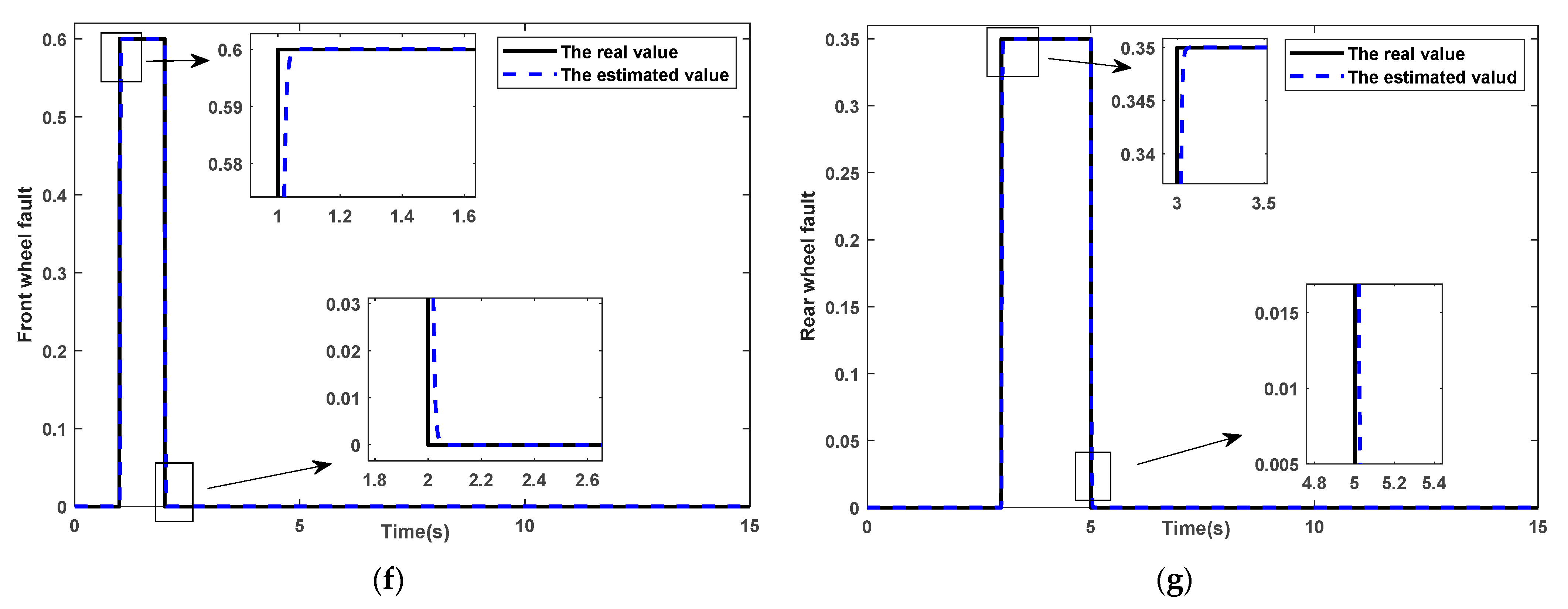
We now consider the situation when the system suffers an actuator fault. When driving at a high speed, the steering wheel vibrates, and the car is not stable. When the steering wheel jitters seriously, there is a feeling of shaking hands. The continuous vibration of the vehicle will cause periodic fault of the actuator. Vehicle parts aging and poor contact will also produce intermittent fault. We assume that the front wheel is with fault in the time interval of 1 s–2 s, while the rear wheel is with fault in the time interval of 3 s–5 s, respectively. The specific fault values are assumed to be as follows:
f a f 1 = { 0.6 1 t 2 s 0 o t h e r s f a r 1 = { 0.35 3 t 5 s 0 o t h e r s
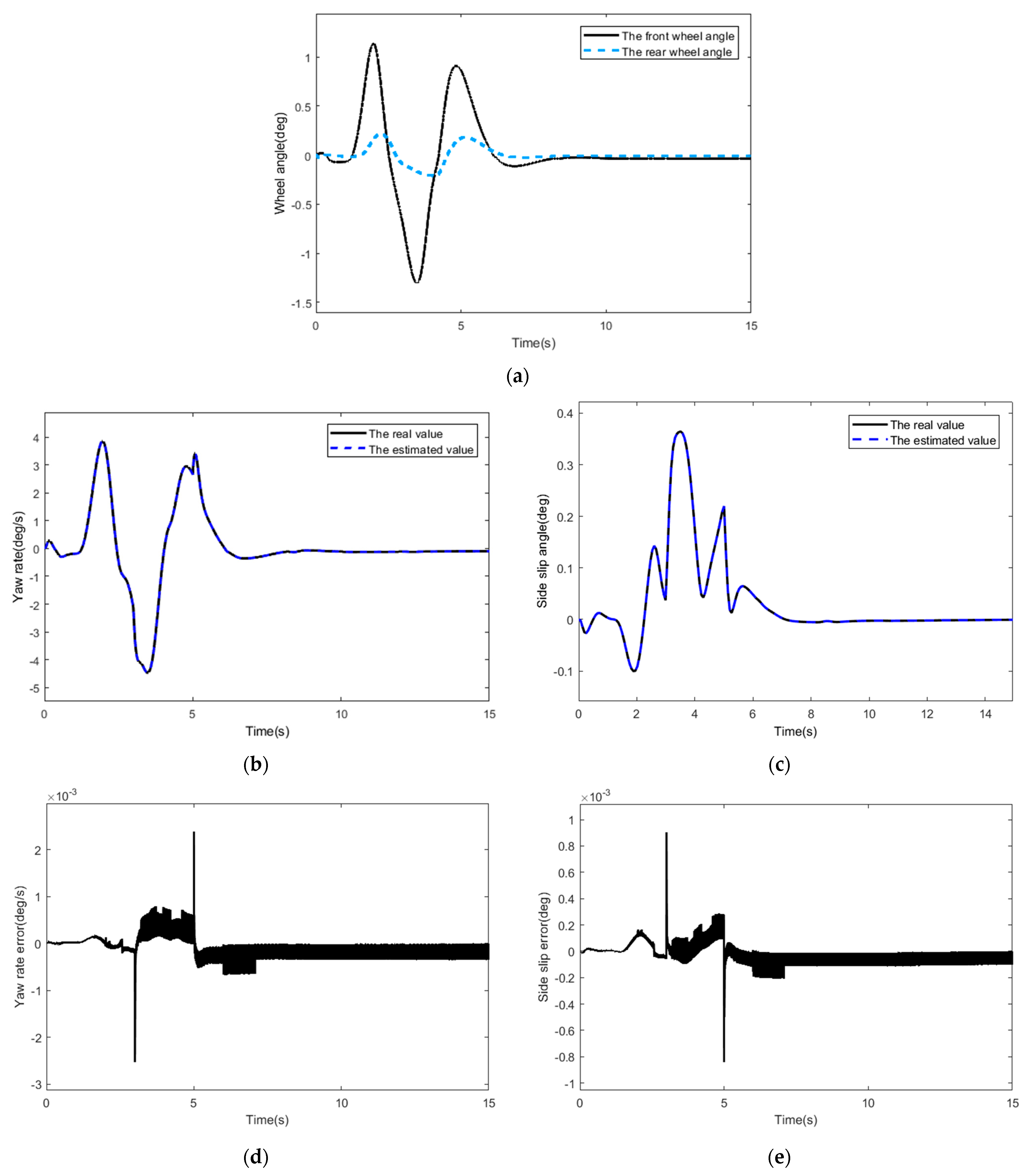
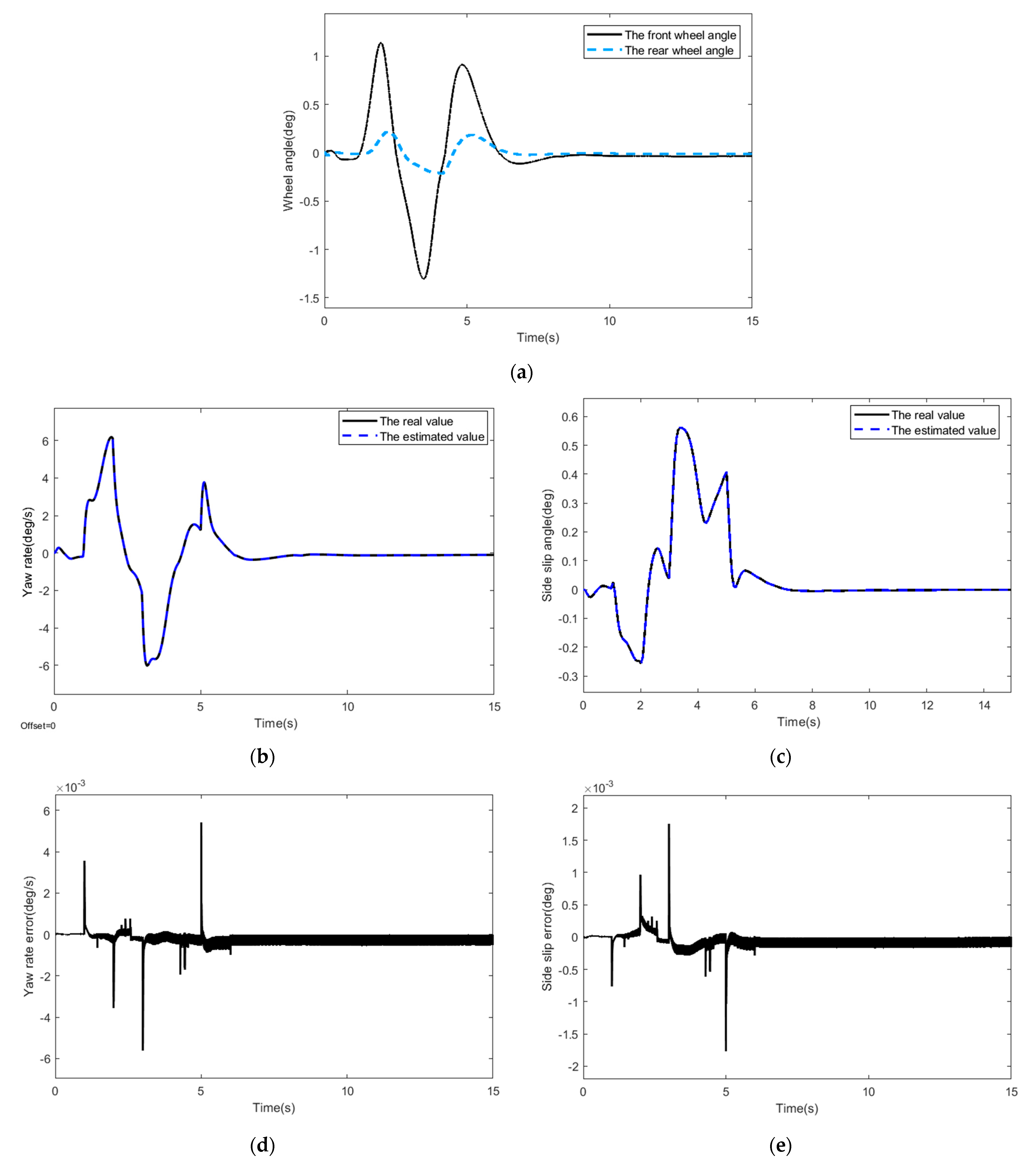
The simulation results are shown in Figure 2.
Figure 2a shows curves of the front and rear wheel angles of the vehicle when driving under double lane change conditions. The curves of yaw rate and side slip angle are shown in Figure 2b,c, respectively. It can be seen from Figure 2b,c that the designed observer can well estimate the yaw rate and side slip angle when the vehicle is driving on an ordinary road surface, and they finally stabilize at zero. Figure 2d,e shows the error curves of the yaw rate and side slip angle, respectively.
The variation trend of the front wheel angle is basically consistent with the driving path, and there is no large deviation. The absolute value of the side slip angle of the four-wheel steering vehicle can be maintained around 6 deg/s. In the case of sudden actuator fault at 1 s and 3 s, there are obvious errors between the estimated the yaw rate and side slip angle and the real value, but the estimated value can quickly track the real value. It can be seen from Figure 2d,e that the yaw rate error is within 0.006 deg/s, and the side slip angle error is within 0.002 deg, respectively. The estimation of the yaw rate and the side slip error are within the acceptable error range, which indicates that the designed observer has strong robustness. Figure 2f,g shows the estimated and real fault curves of the front and rear wheel of the vehicle, respectively, to realize the reconstruction of actuator faults and achieve the purpose of fault diagnosis. In addition, it can be seen from the figure that the designed method can diagnose faults in real time when faults occur. As can be seen from the Figure 2, the vehicle can respond in real time, and the yaw rate is controlled to prevent vehicle instability.

4.1.2. Fault Occurs at the Same Time

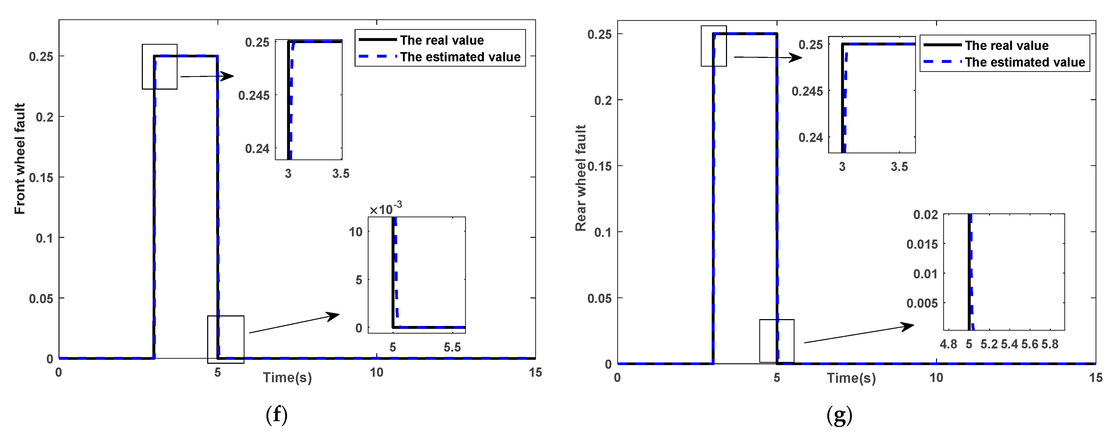
We now consider the situation when the front wheel and the rear wheel of the actuator fail in seconds 3~5 s. The specific fault values are assumed to be as follows:
f a f 2 = { 0.25 3 t 5 s 0 o t h e r s f a r 2 = { 0.25 3 t 5 s 0 o t h e r s
In the same working condition, both front and rear wheels fail simultaneously. The simulation results are shown in Figure 3.
Figure 3a shows the angle curve of the front and rear wheels of the vehicle. Figure 3b,c shows the curves of the yaw rate and side slip angle of the vehicle. The state estimation error curves are given in Figure 3d,e. The actuator faults estimations are shown in Figure 3f,g.
Under double lane change conditions, the vehicle drives through the specified lane without touching the lane line. During the whole test process, the specified speed should be kept constant, and the vehicle can respond to different steering inputs in real time. When the front and rear wheels fail simultaneously, we can reconstruct the faults. In the case of fault from 3 s to 5 s, the estimated value and the true value of the vehicle parameters quickly can maintain the stability of the vehicle. Before 8 s, there will be a slight yaw of the body, but it will not affect the occurrence of sideslip rollover of the vehicle.
As can be seen from Figure 2 and Figure 3, the performance of the proposed method is satisfactory. According to the simulation results, it can be seen that the designed fault diagnosis strategy not only can detect the fault of the actuator but also has a good estimation effect.

4.2. Slippery Road Surface ( u = 80   k m / h and μ = 0.5 )

In order to simulate the observation effect under a variety of complex conditions and more accurately analyze the operation stability of the vehicle under the extreme conditions, we carried out double line change simulation on slippery road conditions. The contact area of the tire and the road surface is reduced, the adhesion decreases more, and it is easy to skid, causing traffic accidents.
In this simulation, the vehicle speed is given as u = 80   k m / h , and the road adhesion coefficient is chosen as μ = 0.5 ; other simulation conditions are the same. We obtain the following state-space matrices corresponding to the model in (15):
A ¯ = [ A E a 0 0 ] = [ 12 . 9674 91 . 1170 56 . 5705 147 . 6875 0 . 7794 8 . 0816 2 . 9953 5 . 0863 0 0 0 0 0 0 0 0 ] ,   B ¯ = [ B 0 ] = [ 56 . 5705 147 . 6875 2 . 9953 5 . 0863 0 0 ] ,   C ¯ = [ C 0 ] = [ 1 0 0 0 0 1 0 0 0 0 1 0 0 0 0 1 ]
The YALMIP toolbox is used to solve the linear matrix inequality, and the observer gain L 2 is finally obtained.
L 2 = [ 3613 . 92 273 . 34 28.29 73.84 143 . 33 1321 . 94 1 . 50 2 . 55 0 . 94 0 . 083 119 . 23 0 2 . 47 0 . 46 0 119 . 23 ]
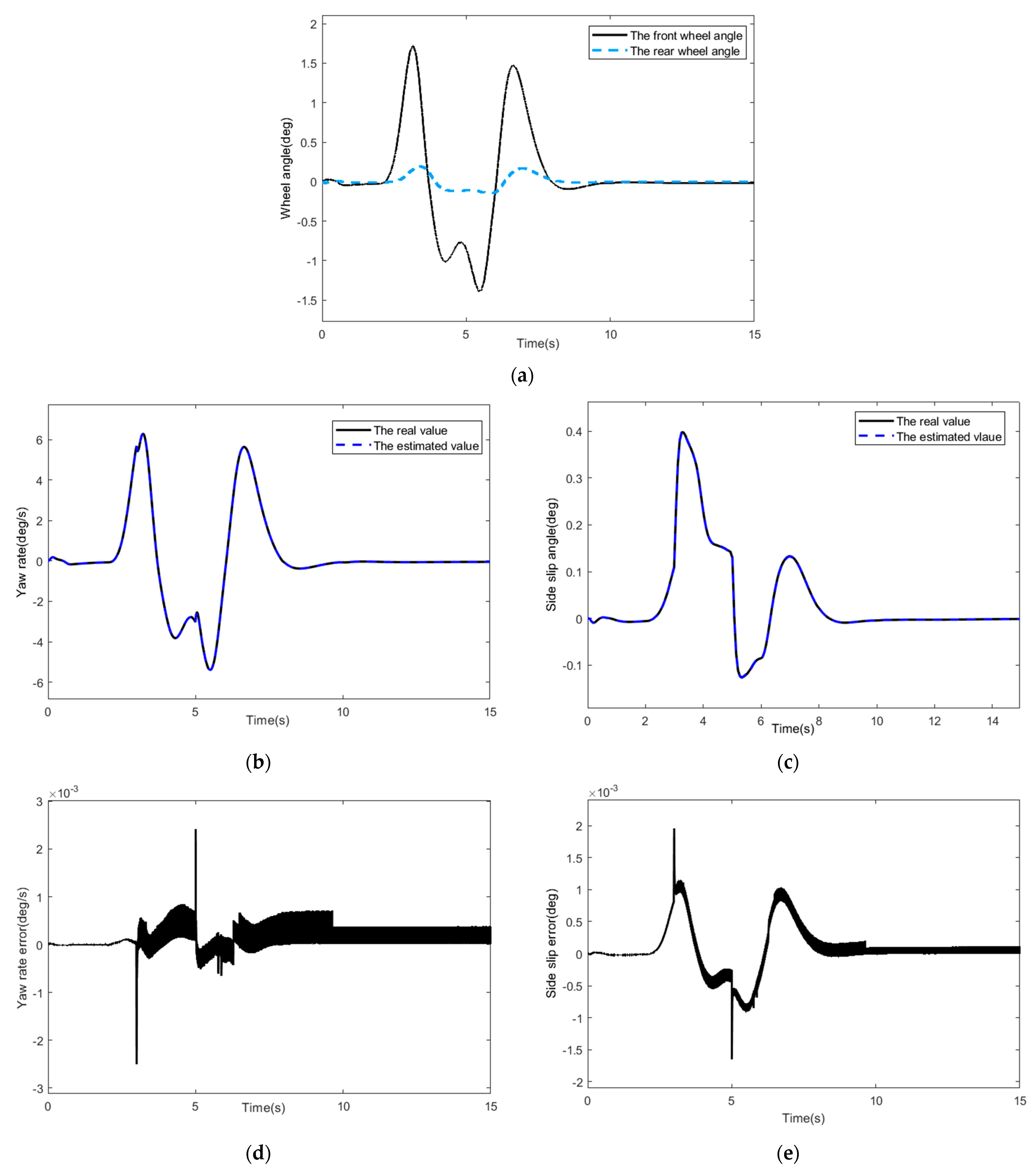
The actuator faults are chosen as f a f 2 and f a r 2 , and the faults occur at the same time. The simulation results are as follows in Figure 4.
In view of the harsh environment on wet roads, the input curves of front and rear wheel angles are shown in Figure 4a. Figure 4b,c shows the curves of the yaw rate and side slip angle of the vehicle. The state estimation error curves are given in Figure 4d,e. The actuator faults estimations are shown in Figure 4f,g.
It can be seen from the Figure 4 that the estimated the yaw rate and side slip angle can track the real value when driving under the condition of double line change on a wet road surface. Under the condition of low adhesion coefficient, the amplitude of the front wheel angle is between −1.5 deg and 1.8 deg. The amplitude of the yaw rate is between −6 deg/s and 6.5 deg/s without understeer or oversteer. The amplitude of the side slip is between −0.15 deg and 0.4 deg and remains at a small value. The vehicle will not deviate too much from the driving direction to ensure the stability of the vehicle. The error between the real value and the estimated value of the real yaw ranges from −0.003 deg/s to 0.003 deg/s. The error between the real value and the estimated value of side slip angle ranges from −0.002 deg to 0.002 deg. When the 3 s fault occurs, there is a significant error between the real value and the estimated value of the yaw rate and side slip angle, but soon the estimated value can track the real value. As the amplitude of the front and rear wheel angle decreases gradually, the yaw rate gradually stabilizes and finally stabilizes near zero value. The simulation results indicate that the scheme can effectively improve the vehicle handling stability on wet roads.
According to the above simulation results, the actuator fault diagnosis can be realized under different working conditions. In the presence of actuator fault and disturbance, the vehicle can drive in the given direction, which effectively verifies that the designed H-infinite observer can suppress the disturbance ability and maintain stable driving. The designed fault diagnosis strategy can estimate actuator faults under various complex conditions, has good robustness and makes preparations for the next fault-tolerant control.
5. Conclusions

In this article, we present an H-infinity observer to diagnose faults for the non-linear vehicle steering system subjected to model uncertainties, unknown disturbances and actuator faults. For the system, a mathematical model of a dual-input dual-output four-wheel steering system is established, and an H-infinity observer is designed to detect the actuator faults in the non-linear uncertain system. The effectiveness of the proposed method is verified by co-simulation with Carsim and MATLAB/ Simulink. The simulation results show that the designed observer has a good observation effect. In the case of vehicle actuator fault, some efforts will be performed to improve the vehicle handling stability by driving in a given straight line or by turning left, etc. When subjected to external interference, the car can resist interference, sideslips rollover does not occur, and the vehicle can quickly restore the original driving state and maintain stable driving performance. The vehicle is simulated on high-speed common road surface and wet road surface, and better estimation results and the fault reconstruction are obtained. The estimation errors of the yaw rate and side slip angle under different complex working conditions are very small, and the yaw rate and side slip angle eventually stabilize to the value of zero. The designed H-infinity observer can not only ensure the robustness and make the system to reach an asymptotically stable state but also increase the accuracy of fault judgment. This method can estimate the original system state and actuator fault separately, and it is convenient for fault-tolerant control. The scheme can be effectively used in the control of vehicle steering system to improve the vehicle handling stability in the case of actuator faults. The proposed scheme can also be generalized for systems containing input delays in the next step.

Author Contributions

Conceptualization, H.W. and Q.W.; methodology, H.W. and Q.W.; software, Q.W., H.Z. and J.H.; validation, H.W.; formal analysis, H.W. and Q.W.; investigation, H.W. and Q.W.; resources, H.W. and Q.W.; data curation, Q.W.; writing—original draft preparation, Q.W.; writing—review and editing, H.W.; visualization, H.W. and Q.W.; supervision, H.Z. and J.H.; project administration, H.W. All authors have read and agreed to the published version of the manuscript.

Funding

This research was funded by the National Natural Science Foundation of China (Grant No. 61903072), Higher Educational Science and Technology Program of Hebei Province (Grant No. QN2019317) and Fundamental Research Funds for the Central Universities (Grant No. N2023018).

Institutional Review Board Statement

Not applicable.

Informed Consent Statement

Not applicable.

Data Availability Statement

The data used in this study are self-text and self-collection.

Conflicts of Interest

The authors declare no conflict of interest.

References

  1. Abzi, I.; Kabbaj, M.N.; Benbrahim, M. Fault tolerant control of vehicle lateral dynamic using a new pneumatic forces multiple model. Actuators 2020, 9, 120. [Google Scholar] [CrossRef]
  2. Balachandran, A.; Gerdes, J.C. Designing steering feel for steer-by-wire vehicles using objective measures. IEEE/ASME Trans. Mechatron. 2014, 20, 373–383. [Google Scholar] [CrossRef]
  3. Sun, Z.; Zheng, J.; Man, Z.; Wang, H. Robust control of a vehicle steer-by-wire system using Adaptive Sliding Mode. IEEE Trans. Ind. Electron. 2015, 63, 2251–2262. [Google Scholar] [CrossRef]
  4. Huang, C.; Naghdy, F.; Du, H. Observer-based fault tolerant controller for uncertain steer-by-wire systems using the delta operator. IEEE/ASME Trans. Mechatron. 2018, 23, 2587–2598. [Google Scholar] [CrossRef]
  5. Wada, N.; Fujii, K.; Saeki, M. Reconfigurable fault-tolerant controller synthesis for a steer-by-wire vehicle using independently driven wheels. Veh. Syst. Dyn. 2013, 51, 1438–1465. [Google Scholar] [CrossRef]
  6. Huang, C.; Naghdy, F.; Du, H. Fault tolerant sliding mode predictive control for uncertain steer-by-wire system. IEEE Trans. Cybern. 2017, 49, 261–272. [Google Scholar] [CrossRef]
  7. Ren, X. Observer design for actuator failure of a quadrotor. IEEE Access 2020, 8, 152742–152750. [Google Scholar] [CrossRef]
  8. Song, S.; Park, J.H.; Zhang, B.; Song, X. Observer-based adaptive hybrid fuzzy resilient control for fractional-order nonlinear systems with time-varying delays and actuator failures. IEEE T. Fuzzy Syst. 2019, 99, 471–485. [Google Scholar] [CrossRef]
  9. Dai, X.; Gao, Z. From model, signal to knowledge: A data-driven perspective of fault detection and diagnosis. IEEE Trans. Ind. Inform. 2013, 9, 2226–2238. [Google Scholar] [CrossRef] [Green Version]
  10. Prakash, O.; Samantaray, A.K.; Bhattacharyya, R. Model-based diagnosis of multiple faults in hybrid dynamical systems with dynamically updated parameters. IEEE Trans. Syst. Man Cybern. Syst. 2019, 49, 1053–1072. [Google Scholar] [CrossRef]
  11. Lin, S.; Mu, D.; Liu, L.; Lei, Y.Q. A novel fault diagnosis method for DC filter in HVDC systems based on parameter identification. IEEE Trans. Instrum. Meas. 2020, 69, 5969–5971. [Google Scholar] [CrossRef]
  12. Gou, B.; Yan, X.; Yang, X.; Wilson, G.; Liu, S.Y. An intelligent time-adaptive data-driven method for sensor fault diagnosis in induction motor drive system. Trans. Ind. Electron. 2019, 66, 9817–9827. [Google Scholar] [CrossRef]
  13. Chen, L.H.; Liu, M.; Shi, Y.; Zhang, H.J.; Zhao, E. Adaptive fault estimation for unmanned surface vessels with a neural network observer approach. IEEE Trans. Circuits Syst. I Regul. Pap. 2021, 68, 416–425. [Google Scholar] [CrossRef]
  14. Habibi, H.; Howard, I.; Fekih, A.; Simani, S. Decoupling adaptive sliding mode observer design for wind turbines subject to simultaneous faults in sensors and actuators. IEEE/CAA J. Autom. Sin. 2021, 8, 837–847. [Google Scholar] [CrossRef]
  15. Gao, K.; Song, J.; Wang, X.; Li, H. Fractional-order proportional-integral-derivative linear active disturbance rejection control design and parameter optimization for hypersonic vehicles with actuator faults. Tsinghua Sci. Technol. 2021, 26, 9–23. [Google Scholar] [CrossRef]
  16. Yu, M.; Lu, H.; Wang, H.; Xiao, C.; Lan, D. Compound fault diagnosis and sequential prognosis for electric scooter with uncertainties. Actuators 2020, 9, 128. [Google Scholar] [CrossRef]
  17. Wang, J.; Pei, H.; Wang, N. Adaptive output feedback control using fault compensation and fault estimation for linear system with actuator failure. Int. J. Autom. Comput. 2013, 10, 463–471. [Google Scholar] [CrossRef] [Green Version]
  18. Zhu, F.; Shan, Y.; Tang, Y. Actuator and sensor fault detection and isolation for uncertain switched nonlinear system based on sliding mode observers. Int. J. Control Autom. 2021, 19, 3075–3086. [Google Scholar] [CrossRef]
  19. Wang, D.; Bao, Y.; Zhang, X. Fault diagnosis and estimation of actuator and sensor for vehicle stability control system. Process Autom. Instrum. 2017, 38, 41–45. [Google Scholar]
  20. Li, K.; Guo, J.; Luo, Y. Design of robust output-feedback-based automatic steering controller for unmanned electric vehicles. Int. J. Veh. Des. 2019, 79, 63. [Google Scholar] [CrossRef]
  21. Ni, J.; Hu, J.; Xiang, C. Control-configured-vehicle design and implementation on x-by-wire electric vehicle. IEEE Trans. Veh. Technol. 2018, 67, 3755–3766. [Google Scholar] [CrossRef]
  22. Wang, Q.; Zhao, Y.Q.; Deng, Y.; Xu, H.; Deng, H.; Lin, F. Optimal coordinated control of ARS and DYC for four-wheel steer and in-wheel motor driven electric vehicle with unknown tire model. IEEE Trans. Veh. Technol. 2020, 69, 10809–10819. [Google Scholar] [CrossRef]
  23. Yu, S.; Wang, J.; Wang, Y.; Chen, H. Disturbance observer based control for four wheel steering vehicles with model reference. IEEE/CAA J. Autom. Sin. 2018, 5, 1121–1127. [Google Scholar] [CrossRef]
  24. Hou, Y.; Yang, Y. Research on coordinated stability control of automobile 4WS and ESP system based on road surface. In Proceedings of the 2019 4th International Conference on Electromechanical Control Technology and Transportation (ICECTT), Shenyang, China, 26–28 April 2019. [Google Scholar]
  25. Chen, L.; Li, P.; Lin, W.; Zhou, Q. Observer-based fuzzy control for four-wheel independently driven electric vehicles with active steering systems. Int. J. Fuzzy Syst. 2020, 22, 89–100. [Google Scholar] [CrossRef]
  26. Lee, S.; Yoon, Y.; Park, J.; Hong, W. Control allocation of rear wheel steering and electronic stability control with actuator failure. In Proceedings of the 2018 IEEE International Conference on Vehicular Electronics and Safety (ICVES) IEEE, Madrid, Spain, 12–14 September 2018. [Google Scholar]
  27. Guo, J.; Luo, Y.; Li, K. Robust H∞ fault-tolerant lateral control of four-wheel-steering autonomous vehicles. Int. J. Automot. Technol. 2020, 21, 993–1000. [Google Scholar] [CrossRef]
  28. Guvenc, B.A.; Bunte, T.; Odenthal, D.; Guvenc, L. Robust two degree-of-freedom vehicle steering controller design. IEEE Trans. Control Syst. Technol. 2004, 12, 627–636. [Google Scholar] [CrossRef]
  29. Zhang, H.; Wang, J. Active steering actuator fault detection for an automatically-steered electric ground vehicle. IEEE Trans. Veh. Technol. 2017, 5, 3685–3702. [Google Scholar] [CrossRef]
  30. Guo, B.; Chen, Y. Robust adaptive fault tolerant control of four wheel independently actuated electric vehicles. IEEE Trans. Ind. Inform. 2019, 16, 2882–2894. [Google Scholar] [CrossRef]
  31. Yang, J.; Zhu, F.; Wang, X.; Bu, X. Robust sliding-mode observer-based sensor fault estimation, actuator fault detection and isolation for uncertain nonlinear systems. Int. J. Control Autom. 2015, 13, 1037–1046. [Google Scholar] [CrossRef]
  32. Li, X.; Souza, C.E.D. Criteria for robust stability and stabilization of uncertain linear system with state delay. Automatic 1997, 33, 1657–1662. [Google Scholar] [CrossRef]
Figure 1. Two-degree-of-freedom model of four-wheel steering.
Actuators 11 00043 g001
Figure 2. The response curve of the system. (a) The curve of front and rear wheel angles. (b) The curve of the yaw rate. (c) The curve of side slip angle. (d) The error curve of the yaw rate. (e) The error curve of side slip angle. (f) The curve of front wheel fault. (g) The curve of rear wheel fault.
Actuators 11 00043 g002aActuators 11 00043 g002b
Figure 3. The response curve of the system. (a) The curve of front and rear wheel angle. (b) The curve of the yaw rate. (c) The curve of side slip angle. (d) The error curve of the yaw rate. (e) The error curve of side slip angle. (f) The curve of front wheel fault. (g) The curve of rear wheel fault.
Actuators 11 00043 g003aActuators 11 00043 g003b
Figure 4. The response curve of the system. (a) The curve of front and rear wheel angle. (b) The curve of the yaw rate. (c) The curve of side slip angle. (d) The error curve of the yaw rate. (e) The error curve of side slip angle. (f) The curve of front wheel fault. (g) The curve of rear wheel fault.
Actuators 11 00043 g004aActuators 11 00043 g004b
Publisher’s Note: MDPI stays neutral with regard to jurisdictional claims in published maps and institutional affiliations.