Multi-Disturbance Observers-Based Nonlinear Control Scheme for Wire Rope Tension Control of Hoisting Systems with Backstepping

Abstract

The objective of this paper is to pursue a wire rope control methodology for reducing the tension difference between two wire ropes of a hoisting system. As we know, complicated disturbances exist in the complex electro-hydraulic hoisting system, notably, some of these disturbances are coupled, such as high-speed airflow disturbances, structure vibrations and vibrations in flexible wire ropes. Furthermore, there are model errors in force modeling due to the Coulomb friction between two wire ropes and two moveable head sheaves in the real physical hoisting systems. To eliminate disturbances, two types of disturbance observers (DOs) are employed: a traditional disturbance observer (TDO) and a coupled disturbance observer (CDO), both of which are utilized to estimate and compensate for the Coulomb friction and coupled disturbances online. As a result, a nonlinear backstepping control scheme is presented with estimation values from the TDO and the CDO. The experiment’s results demonstrate the effectiveness of the proposed control methodology.

1. Introduction

Hoisting systems are common wire rope transmission systems that have been widely used in a variety of applications, such as high-speed elevators [1], mine hoisting [2,3], large-scale offshore platforms [4], crawler cranes [5] and so on. Wire ropes are the unique transmission carrier in hoisting systems. It is critical to understand how to guarantee load mass balance in order to reduce the wear and tear of wire ropes, which will prolong the service life of the wire ropes. Both passive and active coordination systems (ACSs) can balance the load mass [2] in wire ropes. To coordinate the wire ropes’ tension, most hoisting systems employ passive devices such as a dancer arm, a hysteresis brake, or two suspended hydraulic cylinders with a communication vessel [2,6]. However, as the hoisting velocity increases, these passive devices are no longer adequate for quick response to multi-wire ropes’ tensions [6,7]. The ACS, on the other hand, is faster and more efficient than passive coordination systems [3]. Additionally, the ACS, combining some active control methodologies, can ensure load balance among multi-wire ropes [8], thereby extending the service life of wire ropes and reducing wire rope vibrations [9].

Without the ACS model, a proportional-integral (PI) controller can coordinate wire rope tensions [10]. However, the PI controller’s performance is never satisfactory. For instance, in Refs. [2,8], PI controllers are conducted on electro-hydraulic servo systems to actively coordinate two wire rope tensions. However, tension differences between two wire ropes are bigger than the model-based control schemes. Therefore, many model-based controllers are meant to produce higher performance by developing the ACS model. Adaptive controllers [11,12,13], robust controllers [14,15,16], and sliding mode controllers [17,18,19,20] are among the approaches developed. Adaptive controllers employ online parameter update approaches or neural network-based adaptive techniques to derive the projection mapping between the adaptive law and some state variables. Robust controllers are designed using MATLAB or other comparable software with linear matrix inequation tools to make them robust to lumped system uncertainties, including disturbances and parameter uncertainties. Sliding mode controllers can be created by employing different sliding mode surfaces to achieve various control goals. All of these controllers are capable of coordinating wire rope tensions. Backstepping controllers (BCs) can be developed by dividing a system state space model into several subsystems, enabling virtual control laws and the real control law to be derived if proper Lyapunov functions are defined according to control goals [21,22,23,24]. Since backstepping techniques deeply analyze the system model, controllers based on backstepping techniques exhibit better performance than the controllers mentioned previously.

However, hoisting systems are mostly employed in challenging environments, many of which will provide complicated disturbances such as high-speed airflow disturbances, structural vibrations, and vibrations in flexible wire ropes, all of which result in difficulties for control performance. Disturbance observers (DOs) are effective tools for dealing with disturbances [25,26], as evidenced by types of DOs such as extended DOs [27], high-gain DOs [21], sliding mode DOs [28,29] and traditional disturbance observers (TDOs) [30,31,32]. What’s more, estimation values from these DOs can be employed in controllers including sliding mode controllers [33,34,35] and backstepping controllers [24,36] to achieve better performance. However, if a system in severe environments has n actuators (n ≥ 2), coupled disturbances will be broadcast throughout a mechanical network of n actuators, which will amplify the effect of coupled disturbances. DOs mentioned above are unsatisfactory to cope with coupled disturbances. As a result, Guo [37] addressed the CDO for multi-electro-hydraulic actuator systems and provided an excellent solution for coupled disturbance suppression. Combining the estimation value of the CDO, backstepping controllers can be derived.

Inspired by the above research, a new model and control approach is proposed for tension coordination of the ACS to achieve noncoupled and coupled disturbances suppression. The main contributions of the paper can be summarized as:

(1)

A differentiable tension model suited for nonlinear control is developed by taking the force model errors into account. By considering coupled disturbances in two hydraulic actuators, a differentiable speed model representing the transmission properties of coupled disturbances is established. Finally, a novel model for the ACS is derived by considering the noncoupled and coupled disturbances.

(2)

To mitigate the detrimental impact of noncoupled and coupled disturbances, a TDO and a CDO are proposed to estimate the nonlinear mapping element of the model and compensate for nonlinear uncertainty, resulting in a smaller tension difference.

(3)

To combine the TDO and the CDO with the backstepping controller, the tension derivative is chosen as the ACS’s state variable to release the displacement term. To demonstrate the stability of the proposed control method, proper Lyapunov functions are developed.

(4)

To verify the proposed control methodology, a series of experimental studies are conducted on the experimental test rig. Comparative experimental results show that the proposed controller exhibits a better performance than a CDO based BC, a TDO based BC, a BC, or a conventional PI controller.

The remainder of the paper is structured as follows. Problem formulation and preliminaries are addressed in Section 2. The MDOBC is presented in Section 3. Section 4 compares some experimental results. Section 5 summarizes the primary conclusion.

2. Problem Formulation and Preliminaries

As shown in Figure 1, 1 and 2 denote the corresponding active coordination mechanism including the No. 1 hydraulic cylinder (N1HC), the No. 2 hydraulic cylinder (N2HC), and the No. i moveable head sheave, and the No. i wire rope. The force F_xi is the resultant force of the tension from the vertical side (F_zi) and the tension from the catenary side (F_fi + F_zi).

$$F_{xi}=F_{zi}+\left(F_{zi}+F_{fi}\right)\sin {\gamma }_i,i=1,2.$$

(1)

where, γ_i is the angle between the catenary wire rope and the upper plane and ${\gamma }_i\in \left[0,\pi /2\right]$ and F_xi is the force of the No. i hydraulic cylinder. F_zi is the No. i wire rope tension. According to Hooke’s law [38],

$$F_{xi}=k_f{x}_{pi}-k_f{x}_{pfi}$$

(2)

where, k_f is the stiffness, x_pi is the displacement of the No. i hydraulic cylinder, x_pfi is the displacement of the No. i movable head sheave. The time derivative of Equation (1) yields

$${\dot{F}}_{zi}=k_f\left({\dot{x}}_{pi}-{\dot{x}}_{pfi}\right)/\left(1+\sin {\gamma }_i\right)+{\Delta }_i$$

(3)

where, ${\Delta }_i=-{\dot{F}}_{fi}\sin {\gamma }_i/\left(1+\sin {\gamma }_i\right)$. If one considers the force balance in two hydraulic cylinders, one can derive the following equation.

$$A_p{P}_{Li}-F_{zi}\left(1+\sin {\gamma }_i\right)=m_i{\ddot{x}}_{pi}+B_{pi}{\dot{x}}_{pi}+m_i{d}_{hi}$$

(4)

where, A_p is the effective area, P_Li = p_i1 − p_i2 is the load pressure, m_i is the load mass, B_pi is the damping coefficient, d_h1 = (F_f1sinγ₁ + F_g1)/m₁ + d₁₂, d_h2 = (F_f2sinγ₂ + F_g2)/m₂ + d₂₁, d_hi is the total disturbance and d₁₂ and d₂₁ are the coupled disturbances. The load flow Q_Li yields

$$Q_{Li}=A_p{\dot{x}}_{pi}+V_{ti}{\dot{P}}_{Li}/4{\beta }_e+C_{tli}{P}_{Li}$$

(5)

where, C_tli is the total leakage coefficient and V_ti is the total volume. Generally, the load flow Q_Li = (Q_1i + Q_2i)/2 is controlled by the spool displacement x_vi of the corresponding servo valve; therefore,

$$Q_{Li}=C_d\mathrm{w}{x}_{vi}\sqrt{\left(p_s-\mathrm{sign}(x_{vi})P_{Li}^{}\right)/{\rho }_o}.$$

(6)

where, C_d is the discharge coefficient, w is the throttle area gradient, ρ_o is the density of the supply oil and p_s is the supply pressure. According to Ref. [24], the control voltage for the servo valve yields

$$u_{Li}=\sqrt{\Delta p_r/\left(p_s-\mathrm{sign}(Q_{Li})P_{Li}^{}\right)}{u}_{\max }{Q}_{Li}/Q_r.$$

(7)

where, u_Li is the control voltage, Q_r is the rated flow under the rated load pressure Δp_r and u_max is the max control voltage. Defining the state variable as ${\mathit{x}}_i={[x_{i1},x_{i2},x_{i3}]}^T={[F_{zi},{\dot{x}}_{pi},P_{Li}]}^T$, the system state representation yields

$$\{\begin{array}{l}{\dot{x}}_{i1}={\theta }_i{x}_{i2}-{\theta }_i{\dot{x}}_{pfi}+{\Delta }_i\\ {\dot{x}}_{i2}={\theta }_{i1}{x}_{i3}-{\theta }_{i2}{x}_{i2}-{\theta }_{i3}{x}_{i1}+d_{hi}\\ {\dot{x}}_{i3}=-{\theta }_{i4}{x}_{i2}-{\theta }_{i5}{x}_{i3}+{\theta }_{i6}{Q}_{Li}\end{array}.$$

(8)

where, θ_i = k_f/(1 + sinγ_i), θ_i1 = A_p/m_i, θ_i2 = B_pi/m_i, θ_i3 = 1/m_i, θ_i4 = 4A_pβ_e/V_ti, θ_i5 = 4C_tliβ_e/V_ti, θ_i6 = 4β_e/V_ti.

Assumption 1.

Wire rope tensions F_zi and, its time derivatives ${\dot{F}}_{zi}$, ${\ddot{F}}_{zi}$ and ${\stackrel{⃛}{F}}_{zi}$ are all bounded.

Assumption 2.

Disturbances Δ_i, d_hi and their first order time derivatives ${\dot{\Delta }}_i$ and ${\dot{d}}_{hi}$ are varying slowly and bounded, i.e., ${\dot{\Delta }}_i\approx 0$, ${\dot{d}}_{hi}\approx 0$, $\left|{\Delta }_i\right|\le {\vartheta }_i$, $\left|d_{hi}\right|\le {\varsigma }_i$, $\left|{\dot{\Delta }}_i\right|\le {\nu }_i$ and $\left|{\dot{d}}_{hi}\right|\le {\upsilon }_i$.

Remark 1.

In this section, we describe a new model for the ACS of the hoisting system. (1) As shown in Equation (3), a differentiable tension model is established by choosing the tension derivative as one of the ACS’s state variables. Moreover, the Coulomb friction and coupled disturbances are specially considered in the model. The noncoupled disturbances mainly exist in the differentiable force model. (2) Coupled disturbances in the ACS are formulated in the differentiable speed model (4), which indicates that disturbances are delivered through vibrations in mechanical structures. With the state-space model of the ACS, the TDO, the CDO as well as the MDOBC will be developed in the next section.

3. Controller Design

3.1. Development of the TDO

Consider the following disturbance observer

$$\{\begin{array}{l}{\widehat{\Delta }}_i={\xi }_i+p\left(x_{i1},x_{i2}\right)\\ {\dot{\xi }}_i=-\frac{1}{{\lambda }_i}\left[{\xi }_i+p\left(x_{i1},x_{i2}\right)\right]+\frac{1}{{\lambda }_i}\left(-{\theta }_i{x}_{i2}+{\theta }_i{x}_{fpi}\right)\end{array}$$

(9)

where, p(x_i1, x_i2) is a function that needs to be designed, λ_i is the control gain, ${\xi }_i$ is an auxiliary variable. In order to make the TDO stable, the function $p\left(x_{i1},x_{i2}\right)$ and the control gain λ_i should satisfy ${\dot{x}}_{i1}/{\lambda }_i=\dot{p}\left(x_{i1},x_{i2}\right)$ [39,40]. Define the estimation error as ${\tilde{\Delta }}_i={\widehat{\Delta }}_i-{\Delta }_i$. The estimation error dynamics yields

$$\begin{array}{l}{\dot{\tilde{\Delta }}}_i={\dot{\widehat{\Delta }}}_i-{\dot{\Delta }}_i={\dot{\xi }}_i+\dot{p}\left(x_{i1},x_{i2}\right)-{\dot{\Delta }}_i\\ =-\frac{1}{{\lambda }_i}\left[{\xi }_i+p\left(x_{i1},x_{i2}\right)\right]+\frac{1}{{\lambda }_i}\left(-{\theta }_i{x}_{i2}+{\theta }_i{x}_{fpi}\right)+\frac{1}{{\lambda }_i}{\dot{x}}_{i1}-0\\ =-\frac{1}{{\lambda }_i}\left[{\xi }_i+p\left(x_{i1},x_{i2}\right)\right]+\frac{1}{{\lambda }_i}\left({\dot{x}}_{i1}-{\theta }_i{x}_{i2}+{\theta }_i{x}_{fpi}\right)\\ =-\frac{1}{{\lambda }_i}{\widehat{\Delta }}_i+\frac{1}{{\lambda }_i}{\Delta }_i=-\frac{1}{{\lambda }_i}{\tilde{\Delta }}_i\end{array}.$$

(10)

Therefore, the function p(x_i1, x_i2) can be designed as

$$p\left(x_{i1},x_{i2}\right)=\frac{1}{{\lambda }_i}{x}_{i1},i=1,2.$$

(11)

With the result of Equation (11), the TDO for the ACS yields

$$\{\begin{array}{l}{\widehat{\Delta }}_i={\xi }_i+\frac{1}{{\lambda }_i}{x}_{i1}\\ {\dot{\xi }}_i=-\frac{1}{{\lambda }_i}\left[{\xi }_i+\frac{1}{{\lambda }_i}{x}_{i1}\right]+\frac{1}{{\lambda }_i}\left(-{\theta }_i{x}_{i2}+{\theta }_i{x}_{fpi}\right)\end{array}.$$

(12)

The stability proof for the TDO is presented in Appendix A.

Remark 2.

As is shown in Equations (3), (4) and (8), disturbances deriving from the Coulomb friction mainly appear in the first-order and second-order equations of the state space model. The section presents a TDO for estimating the disturbances in the first-order equation. The disturbances in the second-order equation will be estimated by the CDO in the next section.

3.2. Development of the CDO

The CDO for the ACS can be presented as [37]

$${\left[\begin{array}{cc}{\widehat{d}}_{h1}& {\widehat{d}}_{h2}\end{array}\right]}^T=\mathit{A}{\left[\begin{array}{cc}{x}_{12}-{\widehat{x}}_{12}& x_{22}-{\widehat{x}}_{22}\end{array}\right]}^T.$$

(13)

where, ${\widehat{d}}_{hi}$ is the estimation value of d_hi, ${\widehat{x}}_{i2}$ is the estimation value of x_i2, A is the control gain matrix of the CDO, A = [k_d11, k_d12; k_d21, k_d22] and, k_d12 and k_d21 are decoupling terms. Note that A is a Hurwitz matrix and that it is dominated by its diagonal elements. Actually, ${\widehat{x}}_{i2}$ are estimation values of x_i2 with the compensation from the CDO.

$$\left[\begin{array}{c}{\dot{\widehat{x}}}_{12}\\ {\dot{\widehat{x}}}_{22}\end{array}\right]=\left[\begin{array}{cccccc}-{\theta }_{13}& {\theta }_{11}& -{\theta }_{12}& 0& 0& 0\\ 0& 0& 0& -{\theta }_{23}& {\theta }_{21}& -{\theta }_{22}\end{array}\right]\left[\begin{array}{cc}{x}_{11}& 0\\ x_{12}& 0\\ x_{13}& 0\\ 0& x_{21}\\ 0& x_{22}\\ 0& x_{23}\end{array}\right]+\left[\begin{array}{c}{\widehat{d}}_{h1}\\ {\widehat{d}}_{h2}\end{array}\right]$$

(14)

The dynamics of the estimation value ${\widehat{d}}_{hi}$ yield

$${\left[\begin{array}{cc}{\dot{\widehat{d}}}_{h1}& {\dot{\widehat{d}}}_{h2}\end{array}\right]}^T=\mathit{A}{\left[\begin{array}{cc}{\dot{x}}_{12}-{\dot{\widehat{x}}}_{12}& {\dot{x}}_{22}-{\dot{\widehat{x}}}_{22}\end{array}\right]}^T.$$

(15)

The estimation error dynamics of the CDO yield

$${\dot{\tilde{d}}}_{hi}=-k_{di1}{\tilde{d}}_{h1}-\cdots -k_{dii}{\tilde{d}}_{hi}+{\dot{d}}_{hi}.$$

(16)

The stability analysis of the CDO is presented in Appendix A.

Remark 3.

It can be seen that the coupled disturbances mainly derive from the Coulomb friction force and the external load force. By adjusting diagonal terms k_d11 and k_d22 in A, the noncoupled disturbances in the differentiable speed model can be compensated. What’s more, the coupled disturbances can be estimated simultaneously by the decoupling terms k_d11 and k_d22 in A. With the estimation values from the CDO, both noncoupled and coupled disturbances can be compensated in the following controller.

3.3. Development of the MDOBC

Based on the state representation, the system tracking error can be presented as

e = [e_i1, e_i2, e_i3], e_i1 = x_i1 − x_ir, e_i2 = x_i2 − α_i1, e_i3 = x_i3 − α_i2, i = 1, 2.

(17)

where, e_i1 is the two-wire rope tension tracking errors, e_i2 is the two displacement velocity tracking errors, e_i3 is the two load pressure tracking errors and α_i1 and α_i2, i = 1, 2. are the virtual control laws.

Theorem. 

Considering the system state representation (8) and estimation values ${\widehat{\Delta }}_i$ and ${\widehat{d}}_{hi}$ from the TDO and the CDO, there exists the following control law (18), which will guarantee that the system tracking error e enters into a bounded hypersphere ball H_r, ∀t > 0.

$$\{\begin{array}{l}{\alpha }_{i1}=\left(-k_{i1}{e}_{i1}+{\theta }_i{\dot{x}}_{pfi}-{\widehat{\Delta }}_i+{\dot{x}}_{ir}\right)/{\theta }_i\\ {\alpha }_{i2}=\left(-k_{i2}{e}_{i2}-{\theta }_i{e}_{i1}^{}+{\theta }_{i2}{x}_{i2}+{\theta }_{i3}{x}_{i1}-{\widehat{d}}_{hi}+{\dot{\alpha }}_{i1}\right)/{\theta }_{i1}\\ Q_{Li}=\left(-k_{i3}{e}_{i3}-{\theta }_{i1}{e}_{i2}+{\theta }_{i4}{x}_{i2}+{\theta }_{i5}{x}_{i3}+{\dot{\alpha }}_{i2}\right)/{\theta }_{i6}\end{array},i=1,2.$$

(18)

where the hypersphere ball H_r can be presented as

$$\begin{array}{l}{H}_r=-{\displaystyle \sum _{i=1}^2{k}_{i1}{\left(e_{i1}^{}-\frac{1}{2k_{i1}}{\tilde{\Delta }}_i^{}\right)}^2}-{\displaystyle \sum _{i=1}^2\left(\frac{1}{{\lambda }_i}-\frac{1}{4k_{i1}}\right){\tilde{\Delta }}_i^2}\\ -{\displaystyle \sum _{i=1}^2{k}_{i3}{e}_{i3}^2}-{\displaystyle \sum _{i=1}^2{k}_{i2}{\left(e_{i2}^{}+\frac{1}{2k_{i2}}{\tilde{d}}_{hi}^{}\right)}^2}-{\displaystyle \sum _{i=1}^2{\delta }_i{\left[{\tilde{d}}_{hi}^{}+\frac{1}{2{\delta }_i}{\dot{d}}_{hi}\right]}^2}+{\displaystyle \sum _{i=1}^2\frac{{\upsilon }_i^2}{4{\delta }_i}}\end{array},i=1,2.$$

(19)

where, ${\delta }_i=k_{dii}-1/4k_{i2}$. Therefore, if the control gains are properly selected as k_ij > 0 (i = 1, 2., j = 1, 2, 3.), $k_{dii}>1/4k_{i2}$ and $1/{\lambda }_i>1/4k_{i2}$, the system tracking error e will enter into a bounded hypersphere ball H_r, ∀t > 0, and holds in H_r, ∀t > t₀. The closed-loop is bounded stable.

Proof. 

The N1HC backstepping iteration. Step 1-1: If the force dynamics in (8) and ${\tilde{\Delta }}_1={\widehat{\Delta }}_1-{\Delta }_1$ are substituted into ${\dot{e}}_{11}={\dot{x}}_{11}-{\dot{x}}_{1r}$, the derivative ${\dot{e}}_{11}^{}$ yields

$${\dot{e}}_{11}^{}={\theta }_1{x}_{12}-{\theta }_1{\dot{x}}_{pf1}+{\widehat{\Delta }}_1-{\tilde{\Delta }}_1-{\dot{x}}_{1r}.$$

(20)

Define a Lyapunov function as ${\chi }_{11}=e_{11}^2/2+{\tilde{\Delta }}_1^2/2$. With e₁₂ = x₁₂ − α₁₁ in (17), one can derive x₁₂ = e₁₂ + α₁₁.The derivative ${\dot{\chi }}_{11}$ can be presented as

$$\begin{array}{l}{\dot{\chi }}_{11}=e_{11}^{}{\dot{e}}_{11}^{}+{\tilde{\Delta }}_1^{}{\dot{\tilde{\Delta }}}_1^{}\\ =e_{11}^{}\left({\theta }_1{x}_{12}-{\theta }_1{\dot{x}}_{pf1}+{\widehat{\Delta }}_1-{\tilde{\Delta }}_1-{\dot{x}}_{1r}\right)+{\tilde{\Delta }}_1^{}{\dot{\tilde{\Delta }}}_1^{}\\ =e_{11}^{}\left({\theta }_1{e}_{12}+{\theta }_1{\alpha }_{11}-{\theta }_1{\dot{x}}_{pf1}+{\widehat{\Delta }}_1-{\tilde{\Delta }}_1-{\dot{x}}_{1r}\right)+{\tilde{\Delta }}_1^{}{\dot{\tilde{\Delta }}}_1^{}\end{array}.$$

(21)

If the virtual control law ${\alpha }_{11}$ in (18) is substituted into (20), one can derive the following equation:

$${\dot{\chi }}_{11}=-k_{11}{e}_{11}^2+{\theta }_1{e}_{11}^{}{e}_{12}-e_{11}^{}{\tilde{\Delta }}_1-{\tilde{\Delta }}_1^2/{\lambda }_1.$$

(22)

Step 1-2: It can be seen that ${\dot{\chi }}_{11}$ (22) contains a cross-multiplying term θ₁e₁₁e₁₂; therefore, in order to eliminate it, define a Lyapunov function as

$${\chi }_{12}={\chi }_{11}+e_{12}^2/2+{\tilde{d}}_{h1}^2/2.$$

(23)

If the speed dynamics in (8) and $d_{h1}={\widehat{d}}_{h1}-{\tilde{d}}_{h1}$ are substituted into ${\dot{e}}_{12}={\dot{x}}_{12}-{\dot{\alpha }}_{11}$, the derivative ${\dot{e}}_{12}$ yields

$${\dot{e}}_{12}^{}={\theta }_{11}{x}_{13}-{\theta }_{12}{x}_{12}-{\theta }_{13}{x}_{11}+{\widehat{d}}_{h1}-{\tilde{d}}_{h1}-{\dot{\alpha }}_{11}.$$

(24)

The time derivative of ${\chi }_{12}$ yields

$${\dot{\chi }}_{12}={\dot{\chi }}_{11}+e_{12}^{}{\dot{e}}_{12}^{}+{\tilde{d}}_{h1}^{}{\dot{\tilde{d}}}_{h1}^{}.$$

(25)

If e₁₃ = x₁₃ − α₁₂ in (17), ${\dot{\chi }}_{11}$ in (22) and ${\dot{\tilde{d}}}_{hi}$ in (16) are substituted into (25), ${\dot{\chi }}_{12}$ can be further presented as

$$\begin{array}{l}{\dot{\chi }}_{12}=-k_{11}{e}_{11}^2-{\tilde{\Delta }}_1^2/{\lambda }_1+{\theta }_1{e}_{11}^{}{e}_{12}+e_{11}^{}{\tilde{\Delta }}_1\\ +e_{12}^{}\left({\theta }_{11}{\alpha }_{12}+{\theta }_{11}{e}_{13}-{\theta }_{12}{x}_{12}-{\theta }_{13}{x}_{11}+{\widehat{d}}_{h1}-{\tilde{d}}_{h1}-{\dot{\alpha }}_{11}\right)\\ -k_{d11}{\tilde{d}}_{h1}^2-k_{d12}{\tilde{d}}_{h1}{\tilde{d}}_{h2}+{\tilde{d}}_{h1}^{}{\dot{d}}_{h1}\end{array}.$$

(26)

If the virtual control law α₁₂ in (17) is substituted into ${\dot{\chi }}_{12}$, one can derive the following equation.

$$\begin{array}{l}{\dot{\chi }}_{12}=-k_{11}{e}_{11}^2-{\tilde{\Delta }}_1^2/{\lambda }_1+{\theta }_{11}{e}_{12}^{}{e}_{13}-k_{12}{e}_{12}^2-e_{12}^{}{\tilde{d}}_{h1}\\ +e_{11}^{}{\tilde{\Delta }}_1-k_{d11}{\tilde{d}}_{h1}^2-k_{d12}{\tilde{d}}_{h1}{\tilde{d}}_{h2}-{\tilde{d}}_{h1}^{}{\dot{d}}_{h1}\end{array}.$$

(27)

Step 1-3: The cross-multiplying term θ₁₁e₁₂e₁₃ in ${\dot{\chi }}_{12}$ (27) can be eliminated by defining a Lyapunov function as

$${\chi }_{13}={\chi }_{12}+e_{13}^2/2.$$

(28)

With the load pressure dynamics in (8) and e₁₃ = x₁₃ − α₁₂ in (17), the time derivative of e₁₃ can be presented as

$${\dot{e}}_{13}^{}=-{\theta }_{14}{x}_{22}-{\theta }_{15}{x}_{23}+{\theta }_{16}{Q}_{L1}-{\dot{\alpha }}_{12}.$$

(29)

Therefore, the derivative ${\dot{\chi }}_{13}$ yields

$$\begin{array}{l}{\dot{\chi }}_{13}={\dot{\chi }}_{12}+e_{13}^{}{\dot{e}}_{13}^{}\\ =-k_{11}{e}_{11}^2-{\tilde{\Delta }}_1^2/{\lambda }_1+e_{11}^{}{\tilde{\Delta }}_1+{\theta }_{11}{e}_{12}^{}{e}_{13}-k_{12}{e}_{12}^2\\ -e_{12}^{}{\tilde{d}}_{h1}-k_{d11}{\tilde{d}}_{h1}^2-k_{d12}{\tilde{d}}_{h1}{\tilde{d}}_{h2}-{\tilde{d}}_{h1}^{}{\dot{d}}_{h1}+e_{13}^{}\left(-{\theta }_{14}{x}_{22}-{\theta }_{15}{x}_{23}+{\theta }_{16}{Q}_{L1}-{\dot{\alpha }}_{12}\right)\end{array}.$$

(30)

With the real control law Q_L1 in (18), ${\dot{\chi }}_{13}$ can be rewritten as

$$\begin{array}{l}{\dot{\chi }}_{13}=-k_{11}{e}_{11}^2-{\tilde{\Delta }}_1^2/{\lambda }_1+e_{11}^{}{\tilde{\Delta }}_1-k_{12}{e}_{12}^2-e_{12}^{}{\tilde{d}}_{h1}-k_{d11}{\tilde{d}}_{h1}^2-k_{13}{e}_{13}^2-k_{d12}{\tilde{d}}_{h1}{\tilde{d}}_{h2}+{\tilde{d}}_{h1}^{}{\dot{d}}_{h1}\\ =-k_{11}\left(e_{11}^2-\frac{e_{11}^{}{\tilde{\Delta }}_1}{k_{11}}\right)-\frac{{\tilde{\Delta }}_1^2}{{\lambda }_1}-k_{12}\left(e_{12}^2+\frac{e_{12}^{}{\tilde{d}}_{h1}}{k_{12}}\right)-k_{d11}{\tilde{d}}_{h1}^2-{\tilde{d}}_{h1}^{}{\dot{d}}_{h1}-k_{13}{e}_{13}^2-k_{d12}{\tilde{d}}_{h1}{\tilde{d}}_{h2}\\ =-k_{11}{\left(e_{11}^{}-\frac{1}{2k_{11}}{\tilde{\Delta }}_1^{}\right)}^2-\frac{{\tilde{\Delta }}_1^2}{{\lambda }_1}+\frac{1}{4k_{11}}{\tilde{\Delta }}_1^2-k_{12}{\left(e_{12}^{}+\frac{{\tilde{d}}_{h1}}{2k_{12}}\right)}^2\\ +\frac{{\tilde{d}}_{h1}^2}{4k_{12}}-k_{d11}{\tilde{d}}_{h1}^2+{\tilde{d}}_{h1}^{}{\dot{d}}_{h1}-k_{13}{e}_{13}^2-k_{d12}{\tilde{d}}_{h1}{\tilde{d}}_{h2}\\ =-k_{11}{\left(e_{11}^{}-\frac{1}{2k_{11}}{\tilde{\Delta }}_1^{}\right)}^2-\left(\frac{1}{{\lambda }_1}-\frac{1}{4k_{11}}\right){\tilde{\Delta }}_1^2-k_{12}{\left(e_{12}^{}+\frac{{\tilde{d}}_{h1}}{2k_{12}}\right)}^2\\ -\left(k_{d11}-\frac{1}{4k_{12}}\right){\left[{\tilde{d}}_{h1}^{}-\frac{1}{2\left(k_{d11}-\frac{1}{4k_{12}}\right)}{\dot{d}}_{h1}\right]}^2+\frac{1}{4\left(k_{d11}-\frac{1}{4k_{12}}\right)}{\dot{d}}_{h1}^2-k_{13}{e}_{13}^2-k_{d12}{\tilde{d}}_{h1}{\tilde{d}}_{h2}\\ =-k_{11}{\left(e_{11}^{}-\frac{1}{2k_{11}}{\tilde{\Delta }}_1^{}\right)}^2-\left(\frac{1}{{\lambda }_1}-\frac{1}{4k_{11}}\right){\tilde{\Delta }}_1^2-k_{13}{e}_{13}^2\\ -k_{12}{\left(e_{12}^{}+\frac{1}{2k_{12}}{\tilde{d}}_{h1}^{}\right)}^2-{\delta }_1{\left[{\tilde{d}}_{h1}^{}-\frac{1}{2{\delta }_1}{\dot{d}}_{h1}\right]}^2+\frac{{\dot{d}}_{h1}^2}{4{\delta }_1}-k_{d12}{\tilde{d}}_{h1}{\tilde{d}}_{h2}\end{array}.$$

(31)

Remark 4.

Note that the uncertain term $k_{d12}{\tilde{d}}_{h1}{\tilde{d}}_{h2}$ contains a disturbance ${\tilde{d}}_{h2}$ from the N2HC. Therefore, one can eliminate it in the following N2HC backstepping iteration.

The N2HC backstepping iteration. Step 2-1: Define the following Lyapunov function as

$${\chi }_{21}=e_{21}^2/2+{\tilde{\Delta }}_2^2/2.$$

(32)

If the force dynamics in (8) and ${\tilde{\Delta }}_2={\widehat{\Delta }}_2-{\Delta }_2$ are substituted into ${\dot{e}}_{21}={\dot{x}}_{21}-{\dot{x}}_{2r}$, the derivative ${\dot{e}}_{21}$ yields

$${\dot{e}}_{21}^{}={\theta }_2{x}_{22}-{\theta }_2{\dot{x}}_{pf2}+{\widehat{\Delta }}_2-{\tilde{\Delta }}_2-{\dot{x}}_{2r}.$$

(33)

Therefore, the derivative ${\dot{\chi }}_{21}$ yields

$$\begin{array}{l}{\dot{\chi }}_{21}=e_{21}^{}{\dot{e}}_{21}^{}+{\tilde{\Delta }}_2^{}{\dot{\tilde{\Delta }}}_2^{}\\ =e_{21}^{}\left({\theta }_2{e}_{22}+{\theta }_2{\alpha }_{21}-{\theta }_2{\dot{x}}_{pf2}+{\widehat{\Delta }}_2-{\tilde{\Delta }}_2-{\dot{x}}_{2r}\right)+{\tilde{\Delta }}_2^{}{\dot{\tilde{\Delta }}}_2^{}\end{array}.$$

(34)

With the virtual control law α₂₁ in (18), therefore,

$${\dot{\chi }}_{21}=-k_{21}{e}_{21}^2+{\theta }_2{e}_{21}^{}{e}_{22}-e_{21}^{}{\tilde{\Delta }}_2-{\tilde{\Delta }}_2^2/{\lambda }_2.$$

(35)

Step 2-2: It can be seen that ${\dot{\chi }}_{21}$ contains a cross-multiplying term θ₂e₂₁e₂₂. Define a Lyapunov function as

$${\chi }_{22}={\chi }_{21}+e_{22}^2/2+{\tilde{d}}_{h2}^2/2.$$

(36)

If the speed dynamics in (8) and $d_{h2}={\widehat{d}}_{h2}-{\tilde{d}}_{h2}$ are substituted into ${\dot{e}}_{22}={\dot{x}}_{22}-{\dot{\alpha }}_{21}$, one can derive ${\dot{e}}_{22}$ yielding

$${\dot{e}}_{22}^{}={\theta }_{21}{x}_{23}-{\theta }_{22}{x}_{22}-{\theta }_{23}{x}_{21}+{\widehat{d}}_{h2}-{\tilde{d}}_{h2}-{\dot{\alpha }}_{21}.$$

(37)

Further, the time derivative of χ₂₂ yields

$$\begin{array}{l}{\dot{\chi }}_{22}={\dot{\chi }}_{21}+e_{22}^{}{\dot{e}}_{22}^{}+{\tilde{d}}_{h2}^{}{\dot{\tilde{d}}}_{h2}^{}\\ =-k_{21}{e}_{21}^2-{\tilde{\Delta }}_{h2}^2/{\lambda }_2+{\theta }_2{e}_{21}^{}{e}_{22}+e_{21}^{}{\tilde{\Delta }}_2-k_{d22}{\tilde{d}}_{h2}^2+{\tilde{d}}_{h2}^{}{\dot{d}}_{h2}-k_{d21}{\tilde{d}}_{h1}{\tilde{d}}_{h2}\\ +e_{22}^{}\left({\theta }_{21}{\alpha }_{22}+{\theta }_{21}{e}_{23}-{\theta }_{22}{x}_{22}-{\theta }_{23}{x}_{21}+{\widehat{d}}_{h2}-{\tilde{d}}_{h2}-{\dot{\alpha }}_{21}\right)\end{array}.$$

(38)

With the virtual control law α₂₂ in (18), ${\dot{\chi }}_{22}$ yields

$${\dot{\chi }}_{22}=-k_{21}{e}_{21}^2-{\tilde{\Delta }}_2^2/{\lambda }_2+{\theta }_{21}{e}_{22}^{}{e}_{23}-e_{22}^{}{\tilde{d}}_{h2}+e_{21}^{}{\tilde{\Delta }}_2-k_{d21}{\tilde{d}}_{h1}{\tilde{d}}_{h2}-k_{d22}{\tilde{d}}_{h2}^2+{\tilde{d}}_{h2}^{}{\dot{d}}_{h2}.$$

(39)

Step 2-3: It can be seen that ${\dot{\chi }}_{22}$ still contains θ₂₁e₂₂e₂₃; therefore, define the following Lyapunov function as

$${\chi }_{23}={\chi }_{22}+e_{23}^2/2.$$

(40)

If the load pressure dynamics in (8) are substituted into ${\dot{e}}_{23}={\dot{x}}_{23}-{\dot{\alpha }}_{22}$, one can derive ${\dot{e}}_{23}$ yielding

$${\dot{e}}_{23}^{}=-{\theta }_{24}{x}_{22}-{\theta }_{25}{x}_{23}+{\theta }_{26}{Q}_{L2}-{\dot{\alpha }}_{22}$$

(41)

With Equation (41), the derivative ${\dot{\chi }}_{23}$ yields

$$\begin{array}{l}{\dot{\chi }}_{23}={\dot{\chi }}_{22}+e_{23}^{}{\dot{e}}_{23}^{}\\ =-k_{21}{e}_{21}^2-\frac{1}{{\lambda }_2}{\tilde{\Delta }}_2^2+{\theta }_{21}{e}_{22}^{}{e}_{23}-e_{22}^{}{\tilde{d}}_{h2}+e_{21}^{}{\tilde{\Delta }}_2-k_{d21}{\tilde{d}}_{h1}{\tilde{d}}_{h2}-k_{d22}{\tilde{d}}_{h2}^2+{\tilde{d}}_{h2}^{}{\dot{d}}_{h2}+e_{23}^{}{\dot{e}}_{23}^{}\\ =-k_{21}{e}_{21}^2-{\tilde{\Delta }}_2^2/{\lambda }_2+e_{21}^{}{\tilde{\Delta }}_2+{\theta }_{21}{e}_{22}^{}{e}_{23}-k_{22}{e}_{22}^2-e_{22}^{}{\tilde{d}}_{h2}-k_{d22}{\tilde{d}}_{h2}^2\\ -k_{d21}{\tilde{d}}_{h1}{\tilde{d}}_{h2}+{\tilde{d}}_{h2}^{}{\dot{d}}_{h2}+e_{23}^{}\left[-{\theta }_{24}{x}_{22}-{\theta }_{25}{x}_{23}+{\theta }_{26}{Q}_{L2}-{\dot{\alpha }}_{22}\right]\end{array}.$$

(42)

With the real control law Q_L2 in (18), ${\dot{\chi }}_{23}$ yields

$$\begin{array}{l}{\dot{\chi }}_{23}=-k_{21}{e}_{21}^2-{\tilde{\Delta }}_2^2/{\lambda }_2+e_{21}^{}{\tilde{\Delta }}_2-k_{22}{e}_{22}^2-e_{22}^{}{\tilde{d}}_{h2}-k_{d22}{\tilde{d}}_{h2}^2-k_{23}{e}_{23}^2-k_{d21}{\tilde{d}}_{h1}{\tilde{d}}_{h2}+{\tilde{d}}_{h2}^{}{\dot{d}}_{h2}\\ =-k_{21}{\left(e_{21}^{}-\frac{1}{2k_{21}}{\tilde{\Delta }}_2\right)}^2+\frac{{\tilde{\Delta }}_2^2}{4k_{21}}-\frac{{\tilde{\Delta }}_2^2}{{\lambda }_2}-k_{22}{\left(e_{22}^{}+\frac{1}{2k_{22}}{\tilde{d}}_{h2}\right)}^2+\frac{1}{4k_{22}}{\tilde{d}}_{h2}^2-k_{d22}{\tilde{d}}_{h2}^2\\ +{\tilde{d}}_{h2}^{}{\dot{d}}_{h2}-k_{23}{e}_{23}^2-k_{d21}{\tilde{d}}_{h1}{\tilde{d}}_{h2}\\ =-k_{21}{\left(e_{21}^{}-\frac{1}{2k_{21}}{\tilde{\Delta }}_2\right)}^2-\left(\frac{1}{{\lambda }_2}-\frac{1}{4k_{21}}\right){\tilde{\Delta }}_2^2-k_{22}{\left(e_{22}^{}+\frac{1}{2k_{22}}{\tilde{d}}_{h2}\right)}^2-\left(k_{d22}-\frac{1}{4k_{22}}\right){\tilde{d}}_{h2}^2\\ +{\tilde{d}}_{h2}^{}{\dot{d}}_{h2}-k_{23}{e}_{23}^2-k_{d21}{\tilde{d}}_{h1}{\tilde{d}}_{h2}\\ =-k_{21}{\left(e_{21}^{}-\frac{1}{2k_{21}}{\tilde{\Delta }}_2\right)}^2-\left(\frac{1}{{\lambda }_2}-\frac{1}{4k_{21}}\right){\tilde{\Delta }}_2^2-k_{22}{\left(e_{22}^{}+\frac{1}{2k_{22}}{\tilde{d}}_{h2}\right)}^2\\ -\left(k_{d22}-\frac{1}{4k_{22}}\right){\left[{\tilde{d}}_{h2}^{}-\frac{1}{\left(k_{d22}-\frac{1}{4k_{22}}\right)}{\dot{d}}_{h2}\right]}^2+\frac{1}{4\left(k_{d22}-\frac{1}{4k_{22}}\right)}{\dot{d}}_{h2}^2-k_{23}{e}_{23}^2-k_{d21}{\tilde{d}}_{h1}{\tilde{d}}_{h2}\\ =-k_{21}{\left(e_{21}^{}-\frac{1}{2k_{21}}{\tilde{\Delta }}_2^{}\right)}^2-\left(\frac{1}{{\lambda }_2}-\frac{1}{4k_{21}}\right){\tilde{\Delta }}_2^2-k_{23}{e}_{23}^2\\ -k_{22}{\left(e_{22}^{}+\frac{1}{2k_{22}}{\tilde{d}}_{h2}^{}\right)}^2-{\delta }_2{\left[{\tilde{d}}_{h2}^{}-\frac{1}{2{\delta }_2}{\dot{d}}_{h2}\right]}^2+\frac{{\dot{d}}_{h2}^2}{4{\delta }_2}-k_{d21}{\tilde{d}}_{h1}{\tilde{d}}_{h2}\end{array}$$

(43)

Note that the term $k_{d21}{\tilde{d}}_{h1}{\tilde{d}}_{h2}$ in ${\dot{\chi }}_{23}$ is employed to eliminate the uncertain term $k_{d21}{\tilde{d}}_{h1}{\tilde{d}}_{h2}$ in ${\dot{\chi }}_{13}$. Since the matrix A is a Hurwitz matrix, k_d12 = −k_d21 and $k_{d21}{\tilde{d}}_{h1}{\tilde{d}}_{h2}+k_{d21}{\tilde{d}}_{h1}{\tilde{d}}_{h2}=0$. Therefore, if the derivative ${\dot{\chi }}_{13}$ (30) is substituted into ${\dot{\chi }}_{23}$ (43), one can obtain the following formula.

$$\begin{array}{l}{\dot{\chi }}_{23}=-{\displaystyle \sum _{i=1}^2{k}_{i1}{\left(e_{i1}^{}-\frac{1}{2k_{i1}}{\tilde{\Delta }}_i^{}\right)}^2}-{\displaystyle \sum _{i=1}^2\left(\frac{1}{{\lambda }_i}-\frac{1}{4k_{i1}}\right){\tilde{\Delta }}_i^2-{\displaystyle \sum _{i=1}^2{k}_{i3}{e}_{i3}^2}}-{\displaystyle \sum _{i=1}^2{k}_{i2}{\left(e_{i2}^{}+\frac{1}{2k_{i2}}{\tilde{d}}_{hi}^{}\right)}^2}\\ -{\displaystyle \sum _{i=1}^2{\delta }_i{\left[{\tilde{d}}_{hi}^{}-\frac{1}{2{\delta }_i}{\dot{d}}_{hi}\right]}^2}+{\displaystyle \sum _{i=1}^2\frac{{\dot{d}}_{hi}^2}{4{\delta }_i}}\underset{=0}{\underbrace{-k_{d21}{\tilde{d}}_{h1}{\tilde{d}}_{h2}-k_{d21}{\tilde{d}}_{h1}{\tilde{d}}_{h2}}}\end{array}.$$

(44)

Since the disturbances are bounded, $\left|{\dot{d}}_{hi}\right|\le {\upsilon }_i$, further,

$$\begin{array}{l}{\dot{\chi }}_{23}\le -{\displaystyle \sum _{i=1}^2{k}_{i1}{\left(e_{i1}^{}-\frac{1}{2k_{i1}}{\tilde{\Delta }}_i^{}\right)}^2}-{\displaystyle \sum _{i=1}^2\left(\frac{1}{{\lambda }_i}-\frac{1}{4k_{i1}}\right){\tilde{\Delta }}_i^2-{\displaystyle \sum _{i=1}^2{k}_{i3}{e}_{i3}^2} }\\ -{\displaystyle \sum _{i=1}^2{k}_{i2}{\left(e_{i2}^{}+\frac{1}{2k_{i2}}{\tilde{d}}_{hi}^{}\right)}^2}-{\displaystyle \sum _{i=1}^2{\delta }_i{\left[{\tilde{d}}_{hi}^{}-\frac{1}{2{\delta }_i}{\dot{d}}_{hi}\right]}^2}+{\displaystyle \sum _{i=1}^2\frac{{\upsilon }_i^2}{4{\delta }_i}}\end{array}.$$

(45)

There is only one positive definite term $\sum {\upsilon }_i^2/4{\delta }_i$, i = 1, 2. in ${\dot{\chi }}_{23}$, and other terms in ${\dot{\chi }}_{23}$ are all negative definite. Therefore, if sufficient control gains are properly chosen, ${\dot{\chi }}_{23}$ can be guaranteed to be negative definite and the stability of the MDOBC can be guaranteed. □

Remark 5.

The proof for the MDOBC is conducted on the N1HC and the N2HC separately through the backstepping iteration technique. By employing the backstepping iteration with proposed virtual control laws in (18), we eliminate the cross-multiplying terms in the corresponding time derivative of a proper Lyapunov function for each subsystem; subsequently, we derive the final Lyapunov functions for the N1HC and the N2HC, thus the stability of the closed loop is proven with proposed real control laws in (18). Since the coupled disturbances exist in the ACS, the term $k_{d12}{\tilde{d}}_{h1}{\tilde{d}}_{h2}$ in ${\dot{\chi }}_{13}$ should be eliminated by $k_{d21}{\tilde{d}}_{h1}{\tilde{d}}_{h2}$ in ${\dot{\chi }}_{23}$. Therefore, we substitute ${\dot{\chi }}_{13}$ into ${\dot{\chi }}_{23}$ to complete the stability proof for the MDOBC.

Remark 6.

Since there are two Coulomb friction forces between two wire ropes and two moveable head sheaves, and the coupled disturbances will degrade the performance of the ACS, a TDO and a CDO are consequently designed to make online estimates of the disturbances and compensate for them. With those estimation values, a MDOBC is designed to coordinate two wire rope tensions. The coupled elements in the time derivative of ${\dot{\chi }}_{23}$ are eliminated since the CDO control gain matrix A is a Hurwitz matrix.

Remak 7.

According to Assumption 2, disturbances d_hi vary slowly. Therefore, ${\upsilon }_i$ should be a bounded small value, which indicates that other negative terms can hold ${\dot{\chi }}_{23}\le 0$. To summarize the above statement, the MDOBC is stable.

4. Comparative Experimental Study

4.1. The Experimental Test Rig

Figure 2 presents the hoisting system’s experimental test rig. No. 1 and No. 2 denote the No. 1 and the No. 2 wire ropes, as well as their corresponding movable head sheaves, hydraulic cylinders, and winding drums. The mechanical construction is welded on the lower platform. The conveyance with four ears will be hoisted or lowered through four flexible guides, the two ends of which are fastened to the lower and the upper platforms, respectively. Two drums are secured to the upper platform by several screw bolts. Two hydraulic cylinders are positioned vertically so that they can push or pull two movable head sheaves in two stiff guide rails up or down. As a result, the tensions of the two wire ropes will be coordinated to reduce the tension difference. Two winding drums will hoist or lower the conveyance in accordance with the reference six-stage hoisting velocity, which forms a closed-loop with two corresponding encoders.

Table 1. Key structural parameters of the hoisting system.

Parameters	Values	Parameters	Values
Hoisting height	4.5 m	Width	3.4 m
Whole height	7 m	Length	4.4 m
Diameter of head sheave	0.5 m	Dimensions of the conveyance	0.375 × 0.375 × 0.125 m
Hoisting weight	200 Kg	Diameter of two winding drum	0.4 m

shows the key structural parameters of the experimental test rig. The key hydraulic parameters are presented in

Table 2. Key hydraulic parameters of the hoisting system.

Parameters	Values/Unit	Parameters	Values/Unit
Ap	1.88 × 10−3/m2	Vti	0.38 × 10−3 m3
mi	110/Kg	umax	10 V
ΔPr	21 MPa	Ps	15 × 106 Pa
Bpi	25,000 N/(m/s)	Qr	30 L/min
Ctli	6.9 × 10−13 m3/s/Pa	βe	6.9 × 108 Pa

.

Figure 3 presents the real control system. The basic hardware of the real control system mainly consists of a host computer, a target computer, a signal conditioning system, and a sensor measurement system. Control algorithms written in Simulink will be converted into Visual C language and then delivered to the target computer through the Internet with the xPC Target fast prototyping technology. During the hoisting or the lowering stage, the PCI-1716 board will acquire two tension signals, two displacement signals, and four load pressure signals, which will be optimized by the signal conditioning system from 4–20 mA to 2–10 V. Two control signals for two proportional valves and two electro-hydraulic servo valves will be transformed from ±10 V to ±40 mA by the signal conditioning system and then conducted on two winding drums and two hydraulic cylinders. The sampling time of the real-time control system is 1 ms.

4.2. Comparative Experimental Results

In the experimental study, a six-stage hoisting velocity signal in Figure 4 is employed and a [m/s²] denotes the acceleration in the hoisting phase or the lowering phase. The following six cases are considered. Note that all figures present two wire rope tensions with the black line denoting the No. 1 wire rope tension and the red line denoting the No. 2 wire rope tension.

• No controller: Without any A controller, wire rope tensions are presented in Figure 5.
• The PI controller: The PI controller can be expressed as u_Li = K_pi × e + K_IiΣe. e denotes the tension tracking error. Control gains are selected as K_pi = 0.012 and K_Ii = 0.05. The experimental results are presented in Figure 6;
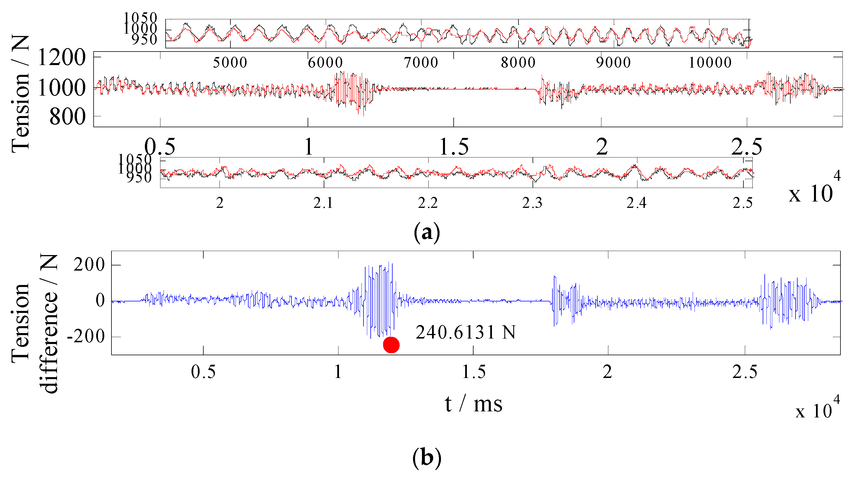
• The BC: With estimation values from the TDO and the CDO being defined as zero, the BC controller is conducted on the ACS. Control gains are selected as k_i1 = 3000, k_i2 = 1000, k_i3 = 1200. The experimental results are presented in Figure 7;
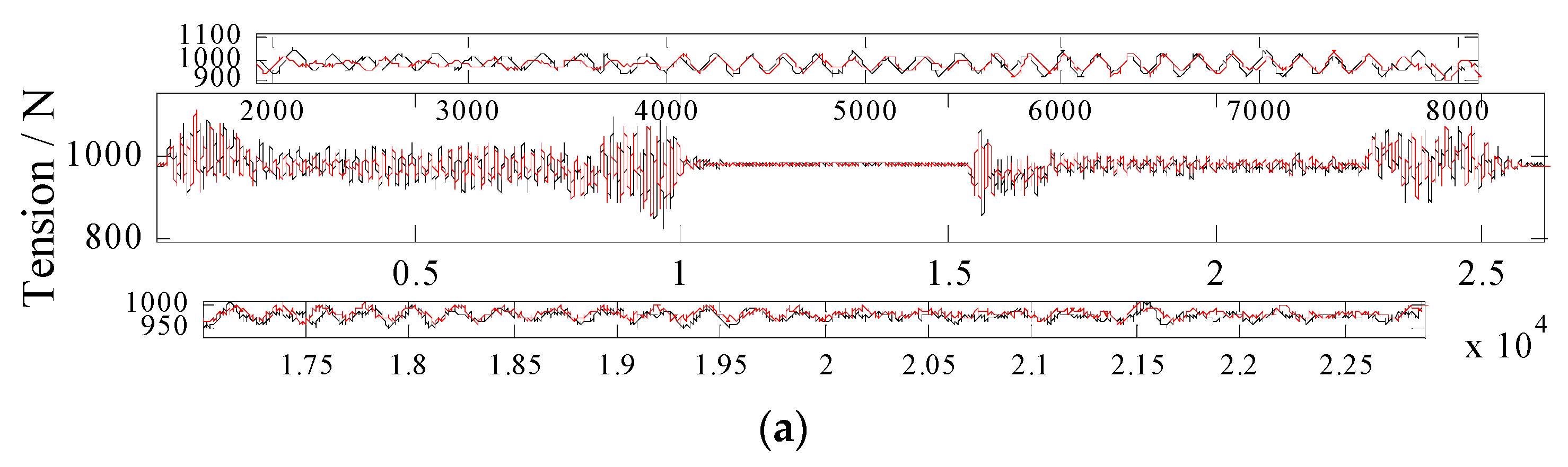
• The TDO based BC: With estimation values from the CDO are defined as zeros, the TDO based BC is conducted on the ACS. Control gains are selected as λ_i = 0.1, k_i1 = 3000, k_i2 = 1000, k_i3 = 1200. Figure 8 presents the experimental results;
• The CDO based BC: With estimation values from the TDO are defined as zeros, the CDO based BC is conducted on the ACS. Control gains are selected as k_d11 = 20, k_d12 = 0.1, k_d21 = 0.1, k_d22 = 20, k_i1 = 3000, k_i2 = 1000, k_i3 = 1200. The experimental results are presented in Figure 9;
• The MDOBC: With the state representation, the MDOBC is designed and conducted on the ACS. Control gains are selected as λ_i = 0.1, k_d11 = 20, k_d12 = 0.1, k_d21 = 0.1, k_d22 = 20, k_i1 = 3000, k_i2 = 1000, k_i3 = 1200. The corresponding experimental results are presented in Figure 10.

The root mean square error (RMSE), employed to illustrate the performance of six controllers, yields

$$\mathrm{RMSE}=\sqrt{{\displaystyle \sum _i^n{\left(R_{in,i}-R_{out,i}\right)}^2}/n}.$$

(46)

where R_in,i denotes the reference signal, R_out,i denotes the feedback signal from the displacement sensor, and n denotes the length of the signal. The RMSE results are presented in

Table 3. The peak error and the RMSE.

Controllers	Peak Error/N	RMSE/N
Without any A controller	417.9225	106.5372
The PI controller	252.2123	38.1489
The BC	240.6131	37.5700
The TDO based BC	219.3711	32.7556
The CDO based BC	208.1213	30.7174
The proposed controller	190.2951	28.2601

.

As illustrated in Figure 5, without any A controller, the tension difference gradually increases in the hoisting stage, then approaches a predetermined value in the stopping stage, and then gradually decreases in the lowering stage. It is obvious that if no controller is utilized, the tension difference is significant. According to Figure 6, when the PI controller is employed, two wire rope tensions are essentially constant; nevertheless, its performance can be improved. Figure 7 presents two tensions of the BC. The vibrations of two wire ropes are decreased, and the performance is superior to that of the PI controller. Due to the complicated disturbances, two tensions are discordant during some time in the hoisting stage or the lowering stage. It can be seen in Figure 8 and Figure 9 that both the TDO based BC and the CDO based BC improve the coordination of two wire ropes. Two tensions with the MDOBC are presented in Figure 10. It can be concluded that the MDOBC can coordinate two wire rope tensions, and the vibrations of two wire ropes are further decreased. Table 3 shows the peak error and the RMSE. One can derive that without any a controller (417.9225 N) > with the PI controller (252.2123 N) > with the BC (240.6131 N) > with the TDO based BC (219.3711 N) > with the CDO based BC (208.1213 N) > with the MDOBC (190.2951 N). The tension difference is reduced from 252.2123 N with the PI controller to 190.2951 N with the MDOBC. The load balance can be further guaranteed so that the wear and tear of the wire ropes will be decreased. From the RMSE analysis, one can derive that without any A controller (106.5372) > the PI controller (38.1489) > the BC (37.5700) > the TDO based BC (32.7556) > the CDO based BC (30.7174) > the MDOBC (28.2601). The RMSE of the tension difference is reduced from 37.5700 RMSE/N with the BC to 28.2601 RMSE/N with the MDOBC, which indicates that both two wire rope tensions’ vibrations are reduced and variations are more consistent. From the above, one can conclude that the performance of the five controllers is as follows: the MDOBC > the CDO based BC > the TDO based BC > the BC > the PI controller.

5. Conclusions

This study is primarily concerned with wire rope tension control methodology for hoisting systems. Since Coulomb frictions between two wire ropes and two corresponding moving head sheaves, as well as complicated coupled disturbances appear in the hoisting system, a novel nonlinear model considering these disturbances is constructed. A TDO and a CDO are designed to online estimate and compensate for them. As a result, a MDOBC is designed to coordinate two wire rope tensions. Comparative experimental results demonstrate that the proposed control methodology exhibits a better performance than the TDO based BC, the CDO based BC, a BC, and a conventional PI controller.

References

1. Tanaka, K.; Nishimura, M.; Wang, H.O. Multi-objective fuzzy control of high rise/high speed elevators using LMIs. In Proceedings of the American Control Conference, Philadelphia, PA, USA, 26 June 1998; pp. 3450–3454. [Google Scholar]
2. Zhu, Z.; Li, X.; Shen, G.; Zhu, W. Wire rope tension control of hoisting systems using a robust nonlinear adaptive backstepping control scheme. ISA Trans. 2018, 72, 256–272. [Google Scholar] [CrossRef] [PubMed]
3. Zang, W.; Shen, G.; Rui, G.; Li, X.; Li, G.; Tang, Y. A flatness-based nonlinear control scheme for wire tension control of hoisting systems. IEEE Access 2019, 7, 146428–146442. [Google Scholar] [CrossRef]
4. Ma, H.; Tang, G.Y.; Hu, W. Feedforward and feedback optimal control with memory for offshore platforms under irregular wave forces. J. Sound Vib. 2009, 328, 369–381. [Google Scholar] [CrossRef]
5. Lee, S.G. Modeling and advanced sliding mode controls of crawler cranes considering wire rope elasticity and complicated operations. Mech. Syst. Signal Process. 2018, 103, 250–263. [Google Scholar]
6. Zhang, D.; Wu, Q.; Yao, X.; Jiao, L. Active disturbance rejection control for looper tension of stainless steel strip processing line. J. Control Eng. Appl. Inform. 2018, 20, 60–68. [Google Scholar]
7. Lu, J.S.; Cheng, M.Y.; Su, K.H.; Tsai, M.C. Wire tension control of an automatic motor winding machine-an iterative learning sliding mode control approach. Robot. Comput. Integr. Manuf. 2018, 50, 50–62. [Google Scholar] [CrossRef]
8. Li, X.; Zhu, Z.; Shen, G. A switching-type controller for wire rope tension coordination of electro-hydraulic-controlled double-rope winding hoisting systems. Proc. Inst. Mech. Eng. Part I J. Syst. Control Eng. 2016, 230, 1126–1144. [Google Scholar] [CrossRef]
9. Chen, X.; Zhu, Z.; Shen, G.; Li, W. Tension coordination control of double-rope winding hoisting system using hybrid learning control scheme. Proc. Inst. Mech. Eng. Part I J. Syst. Control Eng. 2019, 233, 1265–1281. [Google Scholar] [CrossRef]
10. Chen, X.; Zhu, Z.; Li, W.; Shen, G. Fault-tolerant control of double-rope winding hoists combining neural-based adaptive technique and iterative learning method. IEEE Access 2019, 7, 50476–50491. [Google Scholar] [CrossRef]
11. Zhao, J.; Na, J.; Gao, G. Adaptive dynamic programming based robust control of nonlinear systems with unmatched uncertainties. Neurocomputing 2020, 35, 56–65. [Google Scholar] [CrossRef]
12. Sariyildiz, E.; Ohnishi, K. An adaptive reaction force observer design. IEEE/ASME Trans. Mechatron. 2014, 20, 750–760. [Google Scholar] [CrossRef] [Green Version]
13. He, H.; Na, J.; Huang, Y.; Liu, T. Integrated Modeling and Adaptive Parameter Estimation for Hammerstein systems with Asymmetric Dead-Zone. IEEE Trans. Ind. Electron. 2022. [Google Scholar] [CrossRef]
14. Na, J.; Zhao, J.; Gao, G.; Li, Z. Output-feedback robust control of uncertain systems via online data-driven learning. IEEE Trans. Neural Netw. Learn. Syst. 2021, 32, 2650–2662. [Google Scholar] [CrossRef] [PubMed]
15. Sariyildiz, E.; Ohnishi, K. On the explicit robust force control via disturbance observer. IEEE Trans. Ind. Electron. 2014, 62, 1581–1589. [Google Scholar] [CrossRef]
16. Na, J.; Li, Y.; Huang, Y.; Gao, G.; Chen, Q. Output feedback control of uncertain hydraulic servo systems. IEEE Trans. Ind. Electron. 2019, 67, 490–500. [Google Scholar] [CrossRef]
17. Na, J.; He, H.; Huang, Y.; Dong, R. Adaptive estimation of asymmetric dead-zone parameters for sandwich systems. IEEE Trans. Control Syst. Technol. 2021, 30, 1336–1344. [Google Scholar] [CrossRef]
18. Xiao, L.; Lu, B.; Yu, B.; Ye, Z. Cascaded sliding mode force control for a single-rod electrohydraulic actuator. Neurocomputing 2015, 156, 117–120. [Google Scholar] [CrossRef]
19. Roy, S.; Baldi, S.; Fridman, L.M. On adaptive sliding mode control without a priori bounded uncertainty. Automatica 2020, 111, 108650. [Google Scholar] [CrossRef]
20. Wang, J.; Zhu, P.; He, B.; Deng, G.; Zhang, C.; Huang, X. An adaptive neural sliding mode control with ESO for uncertain nonlinear systems. Int. J. Control Autom. Syst. 2020, 19, 687–697. [Google Scholar] [CrossRef]
21. Won, D.; Kim, W.; Shin, D.; Chung, C.C. High-gain disturbance observer-based backstepping control with output tracking error constraint for electro-hydraulic systems. IEEE Trans. Control Syst. Technol. 2014, 23, 787–795. [Google Scholar] [CrossRef]
22. Tee, K.P.; Ge, S.S.; Tay, E.H. Barrier Lyapunov functions for the control of output-constrained nonlinear systems. Automatica 2009, 45, 918–927. [Google Scholar] [CrossRef]
23. He, W.; Sun, C.; Ge, S.S. Top tension control of a flexible marine riser by using integral-barrier Lyapunov function. IEEE/ASME Trans. Mechatron. 2014, 20, 497–505. [Google Scholar] [CrossRef]
24. Zang, W.; Zhang, Q.; Shen, G.; Fu, Y. Extended sliding mode observer based robust adaptive backstepping controller for electro-hydraulic servo system: Theory and experiment. Mechatronics 2022, 85, 102841. [Google Scholar] [CrossRef]
25. Sariyildiz, E.; Oboe, R.; Ohnishi, K. Disturbance observer-based robust control and its applications: 35th anniversary overview. IEEE Trans. Ind. Electron. 2019, 67, 2042–2053. [Google Scholar] [CrossRef] [Green Version]
26. Wei, X.J.; Wu, Z.J.; Karimi, H.R. Disturbance observer-based disturbance attenuation control for a class of stochastic systems. Automatica 2016, 63, 21–25. [Google Scholar] [CrossRef]
27. Kai, G.; Wei, J.; Fang, J.; Feng, R.; Wang, X. Position tracking control of electro-hydraulic single-rod actuator based on an extended disturbance observer. Mechatronics 2015, 27, 47–56. [Google Scholar]
28. Besnard, L.; Shtessel, Y.B.; Landrum, B. Quadrotor vehicle control via sliding mode controller driven by sliding mode disturbance observer. J. Frankl. Inst. 2012, 349, 658–684. [Google Scholar] [CrossRef]
29. Lu, Y.S. Sliding-mode disturbance observer with switching-gain adaptation and its application to optical disk drives. IEEE Trans. Ind. Electron. 2009, 56, 3743–3750. [Google Scholar]
30. Zhang, J.; Liu, X.; Xia, Y.; Zuo, Z.; Wang, Y. Disturbance observer-based integral sliding-mode control for systems with mismatched disturbances. IEEE Trans. Ind. Electron. 2016, 63, 7040–7048. [Google Scholar] [CrossRef]
31. Chen, M.; Shi, P.; Lim, C.C. Robust constrained control for MIMO nonlinear systems based on disturbance observer. IEEE Trans. Autom. Control 2015, 60, 3281–3286. [Google Scholar] [CrossRef]
32. Zheng, M.; Lyu, X.; Liang, X.; Zhang, F. A generalized design method for learning-based disturbance observer. IEEE/ASME Trans. Mechatron. 2021, 26, 45–54. [Google Scholar] [CrossRef]
33. Rashad, R.; El-Badawy, A.; Aboudonia, A. Sliding mode disturbance observer-based control of a twin rotor MIMO system. ISA Trans. 2017, 69, 166–174. [Google Scholar] [CrossRef] [PubMed]
34. Ginoya, D.; Shendge, P.D.; Phadke, S.B. Disturbance observer based sliding mode control of nonlinear mismatched uncertain systems. Commun. Nonlinear Sci. Numer. Simul. 2015, 26, 98–107. [Google Scholar] [CrossRef]
35. Deng, Y.; Wang, J.; Li, H.; Liu, J.; Tian, D. Adaptive sliding mode current control with sliding mode disturbance observer for PMSM drives. ISA Trans. 2019, 88, 113–126. [Google Scholar] [CrossRef] [PubMed]
36. Zhang, C.; Chen, Z.; Wei, C. Sliding mode disturbance observer-based backstepping control for a transport aircraft. Sci. China Inf. Sci. 2013, 57, 1–16. [Google Scholar] [CrossRef] [Green Version]
37. Guo, Q.; Yin, J.M.; Yu, T.; Jiang, D. Coupled-disturbance-observer-based position tracking control for a cascade electro-hydraulic system. ISA Trans. 2017, 68, 367–380. [Google Scholar] [CrossRef] [PubMed]
38. Thompson, J.O. Hooke’s law. Science 1926, 64, 298–299. [Google Scholar] [CrossRef]
39. Chen, W.H.; Yang, J.; Guo, L.; Li, S. Disturbance-observer-based control and related methods—An overview. IEEE Trans. Ind. Electron. 2016, 63, 1083–1095. [Google Scholar] [CrossRef] [Green Version]
40. Chen, W.H.; Ballance, D.J.; Gawthrop, P.J.; O’Reilly, J. A nonlinear disturbance observer for robotic manipulators. IEEE Trans. Ind. Electron. 2000, 47, 932–938. [Google Scholar] [CrossRef]
Figure 1. Schematic diagram of the ACS.
Actuators 11 00321 g001
Figure 2. The experimental test rig.
Actuators 11 00321 g002
Figure 3. The real control system of the hoisting system.
Actuators 11 00321 g003
Figure 4. The six-stage velocity hoisting signal.
Actuators 11 00321 g004
Figure 5. Two wire rope tensions without any A controller: (a) two wire rope tensions; (b) the tension difference.
Actuators 11 00321 g005aActuators 11 00321 g005b
Figure 6. Two wire rope tensions with the PI controller: (a) two wire rope tensions; (b) the tension difference.
Actuators 11 00321 g006
Figure 7. Two wire rope tensions with the BC controller: (a) two wire rope tensions; (b) the tension difference.
Actuators 11 00321 g007
Figure 8. Two wire rope tensions with the TDO based BC controller: (a) two wire rope tensions; (b) the tension difference; (c) the estimation values of Δ1; and (d) the estimation values of Δ2.
Actuators 11 00321 g008aActuators 11 00321 g008b
Figure 9. Two wire rope tensions with the CDO based BC controller: (a) two wire rope tensions; (b) the tension difference; (c) the estimation values of dh1; (d) the estimation values of dh2.
Actuators 11 00321 g009
Figure 10. Two wire rope tensions with the proposed controller: (a) two wire rope tensions; (b) the tension difference; (c) the estimation values of Δ1; (d) the estimation values of Δ2; (e) the estimation values of dh1; and (f) the estimation values of dh2.
Actuators 11 00321 g010