Abstract
In recent years, the lower limb exoskeleton has been more and more widely used in military, medical and other fields. In this paper, the muscle–bone model of the lower limb during the human walking process is analyzed, and a lower limb exoskeleton with the purpose of loadbearing is designed. The exoskeleton is driven by four hydraulic cylinders to the hip and knee joints whose design load is 50 kg. The kinematic and dynamic model of the exoskeleton designed in this paper is established and analyzed, and it is simulated. Finally, the experiments were carried out on the exoskeleton test platform to verify that the stability, bearing capacity, tracking effect and durability of the exoskeleton can meet the requirements.
1. Introduction
An exoskeleton is a wearable intelligent robot device. It integrates multi-disciplinary knowledge such as robotics, mechanism, automatic control principle, artificial intelligence, electrical and electronics, ergonomics and so on. It can enhance the movement ability of bodies. A loadbearing exoskeleton is a kind of exoskeleton. It has very broad application prospects in industrial and military fields. Its related technologies have gradually become a research hotspot for scholars all over the world.
In the industrial field, the earliest industrial exoskeleton was the American “Hardiman” exoskeleton. It was a human enhanced exoskeleton jointly developed by the General Electric Company and Cornell University. The whole weight of the machine is 680 kg with 30 degrees of freedom. The output force can be amplified 25 times at the end of the execution [1]. Fontana developed an exoskeleton robot called “Body Extender”. Its total weight is 165 kg. The wearer can walk at a speed of 1.8 km/h with a load of 100 kg. The whole machine has 22 active joints which are all driven by motor [2]. Although the two exoskeletons above have realized the enhancement of human function, they also have many problems, such as their high weight, large volume, poor movement flexibility, short endurance time and high maintenance cost. The RB3D Company developed an exoskeleton robot called “Hercules”. It is mainly used in fire rescue. The total weight of the exoskeleton is 17 kg. Motors are used to drive hip and knee joints. There are no sensors on the exoskeleton. It uses the control algorithm to judge the motion intention of wearers [3]. Due to the use of a motor for driving, the joint force of Hercules is not very ideal due to the limitation of weight, volume and other factors. The judgement of motion intention is also slightly worse than other exoskeletons using sensors. In recent years, industrial exoskeletons have been applied in batch in automobile manufacturing enterprises. BMW, Ford, Hyundai, Audi and other automobile enterprises have equipped exoskeleton robots for the employees of assembly lines and polishing production lines. This kind of exoskeleton can solve support and power assistance problems. However, there are still many limitations in load bearing and man-machine cooperation [4,5,6,7,8].
In the military field, a loadbearing exoskeleton can significantly improve the load capacity of soldiers. It can effectively improve the delivery capacity of battlefield items and ammunition. In 2004, the University of California at Berkeley developed a lower limb loadbearing exoskeleton called “BLEEX”. Each leg is driven by 4 hydraulic cylinders and has 7 degrees of freedom. The whole weight of the exoskeleton is 41 kg [9,10]. In 2005, Berkeley launched ExoClimber. It is a lower limb loadbearing exoskeleton for long distance walking. The whole weight is 14.1 kg. Soldiers can walk with the exoskeleton at a speed of 4 km/h under a 68 kg load [11]. In order to adapt to stairs and mountainous terrain, Berkeley developed another exoskeleton called “ExoClimber”. The whole weight is 23 kg. Soldiers can easily walk upstairs 183 m with the exoskeleton under a 68 kg load [12]. Due to the powerful function of a military exoskeleton, the United States continues to develop the third-generation military exoskeleton HULC. The weight of HULC is 27.8 kg. Joints are driven hydraulically. It can realize a variety of tactical actions such as loadbearing walking, no-load running and sprint [13]. Raytheon and Lockheed Martin also develop exoskeleton products for the U.S. military. Raytheon’s exoskeleton focuses on a large full-body military exoskeleton [14]. At present, there are still many related studies of the military exoskeleton in progress [15,16,17,18]. However, due to the sensitivity of the military exoskeleton, most of the research and development technologies of the military exoskeleton are not in public. Among the materials that can be searched, the introduction of the military exoskeleton almost describes the basic performance. The reference content is limited.
Although exoskeleton technology has obtained many achievements, the development is still in the primary stage. By summarizing current achievements, there are still some problems existing in the exoskeleton products: (1) Structures of exoskeletons are complex. It makes the whole weight high. Energy consumption is high. (2) The motion prediction system is complex with too many sensors. Maintenance cost is high. (3) The moment provided by exoskeleton joints is not big enough. In order to solve the problems above, a new type of exoskeleton has been designed in this paper. In Section 2, the working principle for muscle and joints during walking is analyzed based on which, the muscle–bone simulation model is established and the walking simulation for human lower limb is conducted, so that the motion angles and torque for lower limb joints are obtained. In Section 3, a novel loadbearing exoskeleton driven hydraulically is proposed, based on the walking principle, and the structure and the sensor system are described in detail. In Section 4, based on the exoskeleton structure, the kinematic model and the dynamic model are set up, and the variation rules of joint torque are calculated by the models. In Section 5, a rigid flexible coupling system of finite element model for the loadbearing exoskeleton is established, which conducts a dynamic finite element simulation of the walking process under load, so that the location of dangerous stress points for exoskeleton parts is obtained. Then, the kinematics simulation for the man–machine coupling system is completed using the man–machine coupling system model in order to check whether the exoskeleton model has motion interference with the human body. In Section 6, the performance tests are conducted to verify the results of theoretical research.
2. Walking Analysis and Muscle–Bone Model Simulation
An exoskeleton is a wearable device that can keep consistent with the movement of human lower limbs. In order to better design the exoskeleton structure, it is significant to analyze the working principle of muscles, bones and joints of the human lower limb in the process of walking. This will guide the design of the exoskeleton structure and control system.
2.1. Walking Analysis
There are three important joints on the human lower limbs. They are the hip joint, knee joint and ankle joint. Both the hip joint and ankle joint have three degrees of freedom. The knee joint is a complex joint. In this paper, it is simplified to one degree of freedom as in other commercial exoskeleton products. The main bone connecting hip joint and knee joint is thighbone. The main bones connecting the knee joint and ankle joint are the tibia and fibula. The bones below the ankle joint are collectively referred to as foot bones. In addition to connecting, the thighbone, tibia, fibula and foot bones are also the main loadbearing bones supporting body weight as shown in Figure 1.
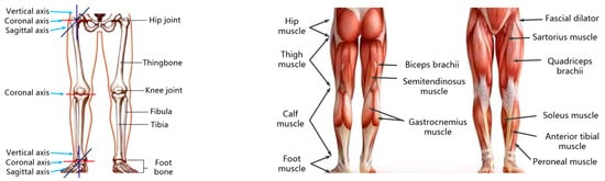
Figure 1.
Bones, joints and muscle diagram of human lower limbs.
The lower limb skeletal muscle consists of hip muscle, thigh muscle, calf muscle and foot muscle. The main function of the anterior group of hip muscles is to make the hip joint into flexion. The posterior group of the hip muscle mainly extends the hip joint and also plays the role of external rotating hip joint. The quadriceps femoris in the anterior group of thigh muscles is for extending the knee joint. Sartorius muscles can make hip and knee joints into flexion. The posterior group of thigh muscles includes biceps femoris, semitendinosus and so on. They have the function of extending the hip joint and flexing the knee joint. The function of the medial group of thigh muscles is to adduct the hip joint. The anterior group of calf muscles includes the anterior tibial muscle, extensor digitorum longus muscle and so on. They can flex the back of the foot. The posterior group of calf muscles includes gastrocnemius and soleus. The main function is to make foot plantar flex, as shown in Figure 1.
The walking process can be divided into swing phase and support phase. They are replaced periodically and alternately. Take the right leg as an example. When the right leg is in the swing phase, the anterior group of hip muscles contract to put the hip joint into flexion. Anterior group of thigh muscles contracts to lift the thigh. The knee joint transits from flexion to extension. The crus kicks forward from the back. The anterior group of calf muscles contracts and the ankle joint is the back extension. Then, the posterior group of hip muscles contracts to extend the hip joint. The posterior group of thigh muscles contracts to make the thigh fall. The knee joint continues to extend. The anterior group of calf muscles stretches. The ankle joint turns from the back extension to plantar flexion. The foot is in contact with the ground. At this time, the right leg changes from the swing phase to the support phase. Then, the posterior group of hip muscles continues to contract and the hip joint continues to extend. The posterior group of thigh muscles contracts to swing the thigh backward. The knee joint changes from extension to flexion. The posterior group of calf muscles contracts. The ankle joint is at plantar flexion. The foot completes the action of pushing backward. At this time, the right leg completes a cycle. The whole process is shown in Figure 2.
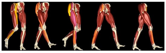
Figure 2.
Schematic diagram of skeletal muscle for human lower limbs.
From the above analysis, it can be seen that the torque applied to joints of lower limbs is related to the degree of expansion and contraction of skeletal muscles of lower limbs. Through the expansion and contraction of skeletal muscles, joints are driven to rotate. Then, lower limb movement is realized and walking action completed.
2.2. Establishment and Simulation of Muscle–Bone Model of Lower Limb
In order to better analyze the motion parameters of human lower limb joints, this paper establishes a muscle–bone simulation model of human lower limbs by using OpenSim. A walking simulation is conducted. OpenSim is open-source human biomechanical analysis software developed by Stanford University. It contains a rich database of human muscle–bone models. It can restore the real data parameters of the human body to the greatest extent. It has been widely used in biomechanics, medical equipment development, orthopedic plastic surgery, rehabilitation medicine and other fields.
When the human body walks forward, the hip joint is mainly flexed and extended. The range of hip rotation and abduction/adduction is relatively small. When establishing the simulation model, this paper only considers flexion and extension in the sagittal plane. The degree of freedom of the hip joint is simplified to 1; the ankle joint is simplified the same as the hip joint. Finally, a single leg is simplified to 3 DOF. Kinematic simulation in OpenSim is mainly to keep the model consistent with the subject’s posture according to the experimental data at each time step. Then, one finishes the simulation of the whole walking process. Muscles are equivalent by the damping spring system as shown in Figure 3.
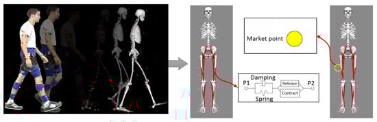
Figure 3.
Simulation principle of muscle bone model.
The model in Figure 3 is a model called “Leg6Dof9Musc.osim” in the OpenSim database. This model has 6 DOF and 9 muscles in a single leg. Three degrees of freedom of the hip joint, knee joint and ankle joint rotating around the coronal axis are needed in this paper: pelvis_ tilt, pelvis_ tx, pelvis_ Ty represent the three degrees of freedom (one rotational degree of freedom and two translational degrees of freedom) of the pelvis in the projection plane in the musculoskeletal model. During the simulation, because the motion of the pelvis in the projection plane is small, the motion of the pelvis is generally not considered. Referring to existing studies, this study ignores the influence of the pelvis, so these three degrees of freedom are not considered, and only the degrees of freedom of the hip joint, knee joint and ankle joint in the projection plane in Figure 4 are considered. Therefore, the three degrees of freedom are fixed in the simulation process. A three-dimensional motion capture system equipped with six infrared cameras is used to collect the kinematic data of fluorescent marker points on human lower limbs during walking. The subject is 180 cm in height and 90 kg in weight. The collected kinematic data are processed into a file format recognized by OpenSim and imported into the software. The default parameters of the software are adopted. The static friction coefficient of the ground is 0.75 and the dynamic friction coefficient is 0.2. The walking speed is 1.125 m/s. Then, a walking simulation is conducted in OpenSim as shown in Figure 4.
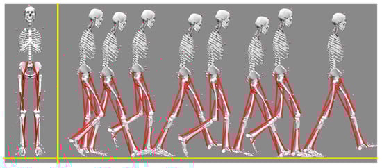
Figure 4.
Walking simulation of muscle–bone model.
During walking progress, the mass center of the human body will fluctuate slightly up and down. Due to the small amplitude, this point is not considered in the later analysis. In the software post-processing module, the curve of the lower limb joint angle changing with time and the curve of the joint torque changing with time can be output as shown in Figure 5.
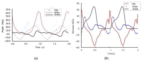
Figure 5.
Curves in sagittal plane: (a) Joint angle and (b) Joint moment.
According to the simulation results, the variation range of the hip angle is 25° to −15°, and the maximum range is 40°. The range of the knee joint angle is 65° to −1°, and the maximum range is 66°. The range of the ankle angle is −8° to 10°, and the maximum range is 18°. The curves in Figure 5 are consistent with the international society of biomechanics [19], the CGA gait database curve of Hong Kong Polytechnic University [20] and the research results of other scholars [21] in terms of magnitude and curve change trend. This proves the correctness of the simulation model and parameter setting.
3. Design for Lower Limb Loadbearing Exoskeleton
Based on the analysis above, this paper proposes a structure design scheme of a loadbearing lower limb exoskeleton. According to the joint drive principle by muscles, a joint drive scheme is proposed. The leg, foot and the whole structure design of the exoskeleton are finished.
3.1. Structure Design
From the aspect of the mechanism, each rotation degree of freedom can be simplified as a planar joint. So, the hip joint, knee joint and ankle joint can be equivalently simplified as shown in Figure 6.
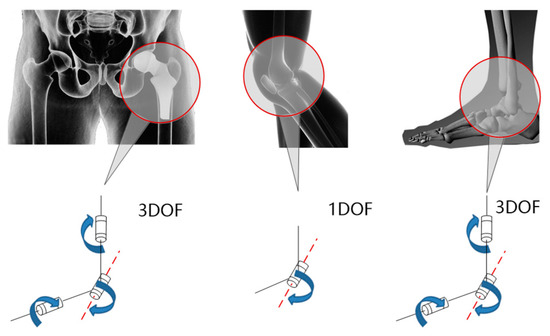
Figure 6.
Joint simplification.
In order to effectively improve joint torque, this paper does not adapt the drive scheme used in the medical exoskeleton: the joint is driven by a frameless torque motor. From the perspective of bionics, this paper uses a hydraulic cylinder to simulate the hip anterior group and thigh anterior group. Hip and knee joints are driven by the push and pull of the cylinders. In order to reduce the complexity of the system and improve the reliability of the system, the ankle joint is designed as a passive joint. The diagram of the exoskeleton driving scheme is shown in Figure 7.
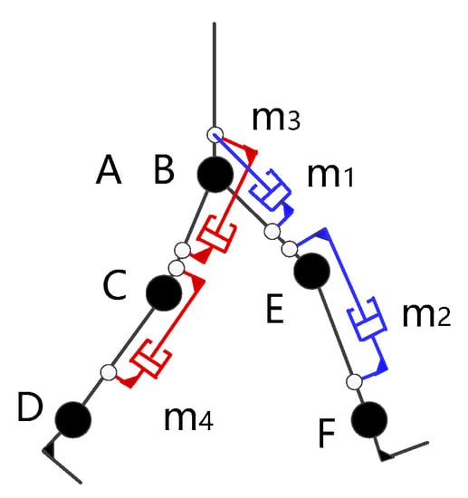
Figure 7.
Driving scheme.
In Figure 7, A and B are two coincident points. They represent the two hip joints. C and D represent the two knee joints. D and F represent the two ankle joints. and are two hydraulic cylinders which drive hip joints. and are two hydraulic cylinders which drive knee joints. According to Figure 6 and Figure 7, a load-bearing exoskeleton structure design is finished as shown in Figure 8.
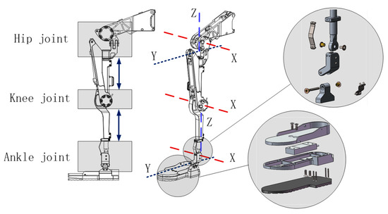
Figure 8.
Structure design.
In the structure in Figure 8, there are three degrees of freedom for the hip joint, one degree of freedom for knee joint and three degrees of freedom for ankle joint. There are seven degrees of freedom in single leg. According to the simulation result in Section 2 and the posture of sitting down, this paper makes a regulation that the angle range for hip joint rotating around the X-axis is . The angle range for the knee joint rotating around the X-axis is . The angle range for the ankle joint rotating around the X-axis is . The angle range for an ankle joint rotating around the X-axis is . Because the ankle joint is designed as a passive joint, this paper uses two spring plates with high stiffness to achieve power assistance. It can also reduce the complex extent and the weight for the whole system. The thigh part is located between the hip joint and the knee joint. The crus part is located between the knee joint and ankle joint. The thigh part and the crus part can adjust their length. The foot structure adopts a multilayer structure. From the bottom to the top of the foot structure, there are the anti-skid rubber, support structure, pressure sensor and trample layer. The pressure sensor is used to collect the plantar pressure of the wearer. Combined with the six-dimensional force sensor information on the back, this can comprehensively judge the wearer’s movement intention. The whole structure of the loadbearing exoskeleton is shown in Figure 9.
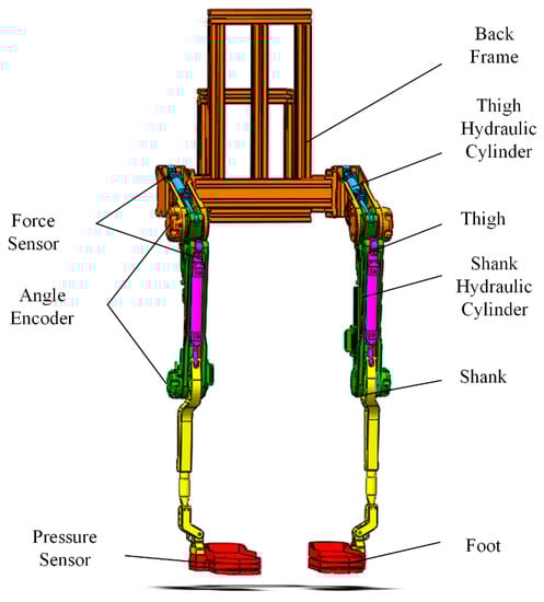
Figure 9.
The whole structure for the exoskeleton.
In Figure 9, the hydraulic cylinder located at the waist side pushes the hip eccentrically to drive the hip rotating. The hydraulic cylinder located in front of the thigh pushes the eccentric wheel of the knee joint to drive the knee joint rotating. Because body size parameters of different wearers are different, the exoskeleton needs to have the function of size adjustment. The exoskeleton designed in this paper is applicable to people whose height is between 1.65 m and 1.80 m. The weight of wears should not be bigger than 90 kg. The maximal load of the exoskeleton is 50 kg. According to GB10000-88, ‘Chinese adult body size’ [22], the design specifications are shown in Table 1.

Table 1.
D-H parameters.
3.2. Design of Motion Judgment System and Hydraulic System
In the control of the exoskeleton in this paper, the wearer’s walking process is divided into two stages: one-foot-support state and two-foot-support state. One-foot-support state means that all loads are placed on the same support leg, the other leg swings; and two-foot-support state support means that the load is shared by both legs. Therefore, each leg of the exoskeleton has three walking states: swing phase, one-foot-support phase and two-foot-support support phase.
The phase switching of the exoskeleton is controlled by two pressure sensors installed in the foot. The pressure sensor has a range of 150 kg, which can meet the walking needs of wearers less than 100 kg. The exoskeleton foot and its sectional view are shown in Figure 10.
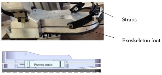
Figure 10.
Exoskeleton foot and its sectional view.
The control method is briefly described as follows: When the plantar pressure is greater than the fixed value a, it is judged as the support phase; when the plantar pressure is less than the value a, it is judged as the swing phase, wherein the value a can be adjusted according to the wearer’s weight and the weight of the load.
Most exoskeletons are driven by hydraulic cylinder, motor, SAE (series elastic actuator), pneumatic muscle and string, etc. Among them, hydraulic drive and motor drive are more widely used. Compared with the motor, the hydraulic cylinder has higher energy density. The exoskeleton designed in this paper is mainly for load bearing, so the hydraulic cylinder has obvious advantages. Therefore, the four active joints of the exoskeleton robot designed in this paper are driven by four hydraulic cylinders. The schematic diagram of the hydraulic system is shown in the Figure 11.
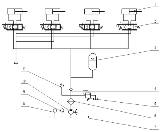
Figure 11.
Schematic diagram of the hydraulic system where 1 is hydraulic cylinder, which contains two knee hydraulic cylinders and two hip hydraulic cylinders, 2 is servo valve, 3 is accumulator used to prevent pressure fluctuation, 4 is one-way valve, which prevents the reverse flow of oil, 5 is overflow valve, 6 is filter, 7 is hydraulic tank, 8 is liquid level gauge, 9 is thermometer, 10 is plunger pump, and 11 is pressure gauge.
According to the position of the hydraulic cylinder, the stroke of the hip hydraulic cylinder is 100 mm and that of the knee hydraulic cylinder is 140 mm. The diameter of the piston rod of the hydraulic cylinder is 10 mm and the diameter of the piston is 20 mm. A precision load cell is installed on the hydraulic cylinder. The knee hydraulic cylinder is shown in Figure 12, and the hip joint hydraulic cylinder is the same as the knee joint hydraulic cylinder except for the stroke length.
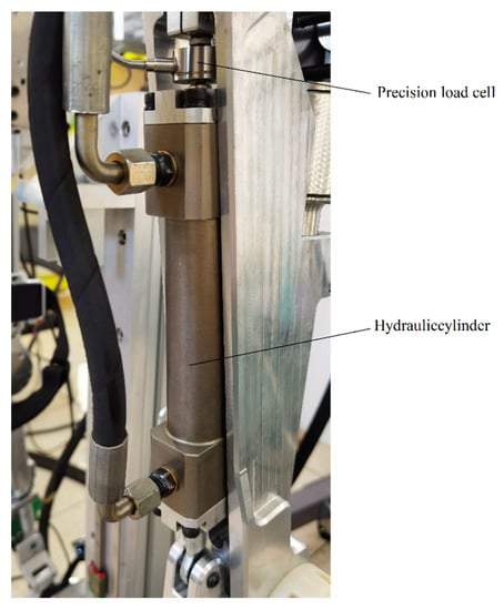
Figure 12.
Knee hydraulic cylinder.
Four FF-102 servo valves are installed side by side on the valve block and connected with the servo valve by hydraulic hoses, as shown in Figure 13. The hoses are short and contain less oil. Therefore, the elastic deformation of the hydraulic oil in the hoses can be ignored in the control process.
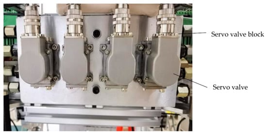
Figure 13.
Servo valve block.
4. Kinematic and Dynamic Analysis of the Exoskeleton
4.1. Kinematic Modelling
In order to simplify the modelling process, trunk, head and upper limbs are regarded as a whole part. The exoskeleton can be simplified into a five-link mechanism as shown in Figure 14. Support phase and swing phase during walking are modelled, respectively. Only the motion in the sagittal plane is considered. The supporting leg can be equivalent to a two-link system in which the foot is connected with the geodetic coordinate system. The swinging leg can be equivalent to a two-link system connected with the waist coordinate system, as shown in Figure 14. According to the D-H method, the axis is the direction along the rotation axis of the joint, and the axis is the direction of the common normal of the adjacent axes.

Figure 14.
Five-link model. is the motion angle for ankle joint. and are motion angles for knee joints. and are motion angles for hip joints. and are the distance between ankle joints and knee joints. and are the distance between knee joints and hip joints. D-H parameters among variables are shown in Table 2.
Table 2.
D-H parameters.
Assuming that the torso part is vertical, so:
The coordinate system fixedly connected to the connecting rod i is called coordinate system {i}. Select the coordinate system fixed on the base as the basic coordinate system. According to the principle of coordinate transformation, it can be seen that:
Therefore, the end position coordinates of the support leg and swing leg can be obtained:
Assume that , .
The expression of each angle can be obtained:
4.2. Dynamic Modelling
The purpose of the dynamic model analysis of the exoskeleton system is to calculate the relationship between the motion state of the system and the joint-driving torque during walking based on the kinematic model. The results can guide the design of the robot driving system and serve as the basis of the robot control of the follow-up force following the control strategy. The common dynamic modeling methods are the Newton–Eulerian method and Lagrangian method, and the Lagrangian method is adopted in this paper. The result of Lagrangian dynamic equation is expressed in the form of matrix, shown as Equation (16).
where , and are the angle, velocity and acceleration of the joint, is an inertia matrix, represents centrifugal force and Coriolis force matrix, is gravity matrix and is the generalized moment of each joint.
Combined with the use scenario of this rehabilitation lower limb exoskeleton robot, similar to the kinematic analysis, the dynamic analysis is only carried out in the sagittal plane. The rehabilitation lower limb exoskeleton robot is simplified into a five-link model for dynamic modeling. Since there are only driving forces at the knee and hip joints in the robot design, only the driving moments of the hip and knee joints are modeled. This simplified model is also applicable to the dynamic modeling of the man–machine integrated system. In order to establish the dynamic model of the robot more accurately, the dynamic model of the support leg and the dynamic model of the swing leg are established, respectively. The support leg is simplified as a three-link model, and the swing leg is simplified as a two-link model. The simplified models are shown in Figure 15.
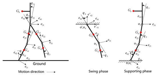
Figure 15.
Simplified structure in sagittal plane.
In Figure 15, and are mass centers of crus. and are mass centers of thighs. Due to the load on the back, the mass center of the trunk is not on the trunk. It will move backward. is the mass center of the trunk. Thigh and crus are simplified as slender uniform linkages. So, mass centers of linkages will locate on the linkages. and . For the swing leg, the initial coordinate O’ is fixed on the hip joint.
According to the Lagrange equation:
The dynamic model of swing leg is shown as:
which can be written in matrix form:
Similarly, the supporting phase dynamics model is as follows ( is not needed in this paper):
4.3. Dynamic Solution
As the exoskeleton is consistent with the lower limb movement of the wearer, the motion angle of the human lower limb is that of the exoskeleton. The motion angle result in Section 2 is brought into the dynamic equation. In the exoskeleton structure model, the mass and length of each component are extracted as shown in Table 3. By bringing the known data into the dynamic equation, the exoskeleton joint torque can be obtained as shown in Figure 16.
Table 3.
The exoskeleton parameters.
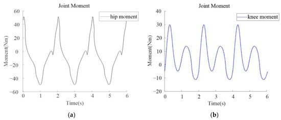
Figure 16.
Moment curves for exoskeleton. (a) Hip joint moment; (b) Knee joint moment.
It can be seen from Figure 16 that the maximum torque of the exoskeleton hip joint is about 50 N·m and that of the knee joint is about 30 Nm. Because the exoskeleton walking is similar to human walking, its joint torque curve should also be similar to the shape of the human joint torque curve. Since the mass of the exoskeleton is 29.08 kg and the maximum load is 50 kg, the weight of the exoskeleton plus the maximum load is 79.08 kg. It is less than the man body quality of the OpenSim simulation in Section 2. Therefore, the maximum torques of the hip and knee joint are smaller than the results in Figure 5b.
5. Finite Element Analysis for Exoskeleton with Rigid Flexible Coupling System
In the previous exoskeleton design process, exoskeleton structural components are generally default to rigid components. However, this treatment deviates greatly from a real situation. Many components have excellent mechanical properties and big flexibility. During the motion process, they will produce large deformation. At this time, if such parts are treated as rigid bodies, accurate analysis results will not be obtained. Therefore, this paper will establish the rigid flexible coupling exoskeleton finite element model. A dynamic finite element analysis of a rigid flexible coupling system is carried out to obtain the maximum stress of exoskeleton parts in a walking cycle. It will be used to verify whether the exoskeleton structure design meets user requirements.
Because elastic parts have great flexibility, in the exoskeleton model, the two high stiffness spring sheets of the ankle joint and the rubber parts of the foot should be treated as flexible bodies. In the joint structure, there is a copper shaft sleeve. The hardness of the copper sleeve is relatively small. When working, its deformation will affect the position of the rotation axis, resulting in the change of joint motion angle. So, it must be treated as a flexible body. In the process of walking, the thigh structure and the crus structure are long. They are the main supporting parts of the exoskeleton. So, the supporting parts of the thigh and crus are treated as flexible bodies.
Establish a transient dynamic analysis project in ANSYS Workbench. Add C45, 7075 aluminum alloy, brass, carbon spring steel, rubber and other materials to the material library. Since these materials are general materials, the material attribute will not be repeated in this paper. Import the loadbearing exoskeleton into the software. Set the material attribute for the parts. All the supporting parts in the exoskeleton adopt 7075 aluminum alloy. All fasteners such as screws are made by C45. The shaft sleeve and bushing are made by brass. All spring plates are made by carbon spring steel. The sole material is rubber. The “stiffness behavior” of the two spring sheets of the ankle joint, the rubber part of the sole, the thigh support part and the crus support part need to be set to “Flexible”, and other components need to be set to “Rigid”. In the item of “Connects”, set the contact of the exoskeleton components. For planar fasteners, add planar contacts. For rotating parts, add rotating pairs. For hydraulic cylinder and push rod, add cylindrical pairs. Then, mesh the loadbearing exoskeleton model, as shown in Figure 17.
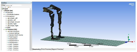
Figure 17.
The setting of the ANSYS model.
In the transient dynamics analysis setting, set the analysis time, the friction coefficient between foot and ground, and turn on the large deformation option. Set the magnitude and direction of gravity acceleration in “Standard Earth Gravity”. Set the rotation range of the hip joint and knee joint. Because most weight is supported by the supporting leg, the dangerous point will happen in the period of the support phase. In order to shorten the simulation time, this paper only simulates one cycle when right leg is in the supporting phase. In support phase, beginning is the maximum angle of hip joint in the backward direction, and the ending is the maximum angle of the hip joint in the forward direction. Accordingly, the knee joint angle can be obtained. Intercept the corresponding part of the joint angle curve obtained in Section 2 and import them into the joint attribute of the hip joint and the knee joint. A 50 kg load is simplified as a remote force in the analysis setup. Its position is 0.1 m behind the waist and 0.2 m above the waist. The load direction is vertical down. Analysis time is 20 s. Basic analysis step is 0.1 s. Others are set by default. Finally, it is solved to obtain the analysis results as shown in Figure 18.
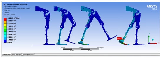
Figure 18.
Stress simulation result of ANSYS.
The simulation results show that when the right leg is used as the supporting leg, a dangerous point of the exoskeleton structure appears at the moment when the left leg is to contact the ground but has not yet contacted. The dangerous point is located on the part connecting the ankle joint and the crus. The maximum stress curve is shown in Figure 19.
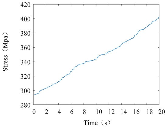
Figure 19.
Maximum stress curve.
From the curve results, it can be seen that at the beginning of the simulation, the maximum stress of the dangerous parts is the smallest in the whole process due to the landing of both feet. With the progress of the simulation, the maximum stress of the dangerous parts gradually increases. When the swing leg is about to land, the maximum stress of the dangerous parts on the support leg reaches the maximum. The maximum stress is 402.92 MPa. The yield limit of 7075 aluminum alloy is 505 MPa. Therefore, the exoskeleton parts meet the use requirements in the structural design.
6. Kinematics and Dynamics Simulation of Exoskeleton with Man–Machine Coupling System
Simple kinematic simulation and dynamic simulation of the exoskeleton can only observe the motion of the exoskeleton. Yet, the real working condition of the exoskeleton is to run with people. Ignoring the existence of human beings and analyzing the exoskeleton alone, the results cannot fully verify the correctness of the exoskeleton design. A man–machine coupling model is established in this paper.
Taking the body parameters of the experimenter in Section 2.2 as an example, the human model is established. The height is 1.80 m. The weight is 90 kg. The length and weight of each part of human is distributed as GB10000-88, ‘Chinese adult body size’ [22]. Take the angles of hip, knee and ankle as the input of the simulation. Then, the dynamic simulation is conducted. A walking animation of the human body is shown in Figure 20.
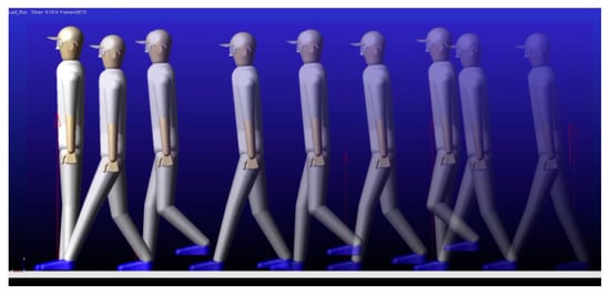
Figure 20.
Dynamic simulation of human body.
After simulation, the post-processing module can output torque data of hip and knee joints. Torque curves of hip and knee joints are drawn by image processing software. The curve is compared with the torque curve obtained by muscle–bone simulation in this paper, as shown in Figure 21.
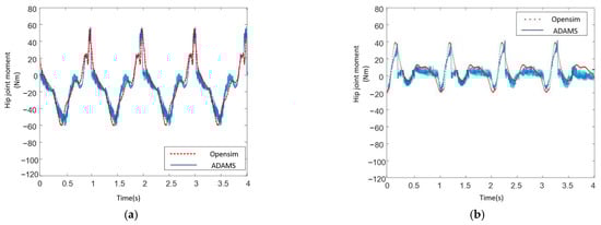
Figure 21.
Simulation curves of human body. (a) hip joint moment curve; (b) knee joint moment curve.
From Figure 21, it can be concluded that the curve gained in ADAMS has the same trend with the curve gained in OpenSim. When simulating in ADAMS, because the model adopts a multi rigid body system, there is instantaneous collision and impact in the simulation process. Therefore, the curve has instantaneous mutation and oscillation. This sudden change of torque caused by the instantaneous collision or impact of rigid bodies does not exist in the real process of human walking, because the human body is a flexible body. Observe the peak and valley values of the curve in Figure 21. Without considering the instantaneous mutation, the magnitude of the simulation results in ADAMS is the same as that in OpenSim. Therefore, considering the curve change trend and the magnitude of the maximum value, the two simulation results are basically consistent. It can indirectly prove that the human model established in this paper is correct. The human model will be used in the simulation of the man–machine coupling system.
Import the exoskeleton 3D model into ADMS. Because the exoskeleton needs to be consistent with the human motion in the process of movement, the motion curves of the human hip and knee are brought into the settings of the exoskeleton hip and knee. The maximum load of the exoskeleton is designed to be 50 kg. So, the mass of the frame behind the exoskeleton is set to 50 kg to be equivalent to the load. Simulate in ADAMS. A simulation animation is obtained in Figure 22.

Figure 22.
Dynamic simulation of the exoskeleton.
After the simulation, torque curves of the exoskeleton hip joint and knee joint are output in the post-processing module. These curves are compared with the curves obtained in Section 4.3 as shown in Figure 23.
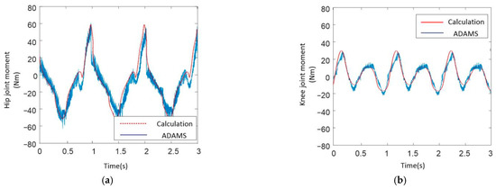
Figure 23.
Simulation curves of exoskeleton. (a) hip joint moment curve; (b) knee joint moment curve.
In Figure 23, there are still transient mutations in the ADAMS simulation curves. This paper has explained the reason above. From the comparison, it can be concluded that the curves obtained by theoretical calculation are nearly the same as the curves obtained by simulation in ADAMS. The shape of the curves is nearly the same. Although there are errors between maximum values and minimum values of the curves, the errors are small. So, it can verify that the theoretical calculation in this paper is correct.
Finally, the human body model is coupled with the exoskeleton model. Set contacts in the foot, legs and waist. The drivers in the human hip joints and knee joints remain. The drivers in the exoskeleton hip joints and knee joints remain. There is interference detection on the human body model. If any parts insert into the human body model during the simulation, there will be an alarm in the system. A simulation animation is shown in Figure 24.
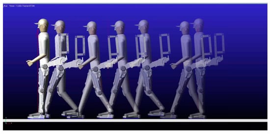
Figure 24.
ADAMS simulation of man–machine coupling system.
During the simulation, there is no alarm given by the system. This shows that there is interference during the walking process. When one man walks with the exoskeleton under a 50 kg load, he just bears his own weight. The exoskeleton will bear the 50 kg load. This can demonstrate that the exoskeleton can effectively improve loadbearing ability.
7. Experimental Verification
In order to verify the correctness of the theoretical research, an experiment prototype is manufactured according to the design scheme. A hydraulic control system and electric system have been set up as shown in Figure 25.
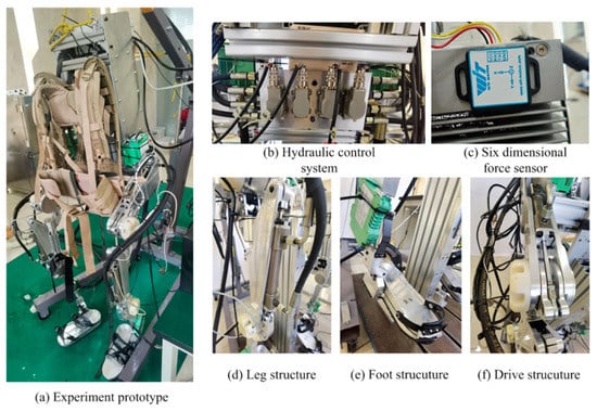
Figure 25.
Experiment prototype.
In Figure 25, the exoskeleton adopts hydraulic drivers. Hydraulic parts are located behind the waist. Each leg has two positive degrees of freedom. There is a pressure sensor under each foot. There is one six-dimension power sensor, a hydraulic oil tank and a 48 V 7 Ah battery in the back framework. The total weight is 33.15 kg. In order to verify the exoskeleton performance, a stability test, a load test, a moment-following test and an endurance test are conducted. Input the motion law of the joint angle during human walking into the controller. It can make the exoskeleton finish circular walking. Due to the long-term uninterrupted test, the battery will not be used as energy in this test.
7.1. Stability Test
Because the exoskeleton is in direct contact with wearers, its stability is very important for the life safety of wearers. In order to verify the stability of the exoskeleton designed in this paper, this paper designs a stability test under the condition of long-time operation. Fix the exoskeleton on the fixed frame. The height of the frame can take the exoskeleton foot away from the ground. A total of 220 V AC is converted to 48 V DC through an adapter to supply power to the exoskeleton. Then, conduct 500 h of an uninterrupted walking test. The test equipment is shown in Figure 26.
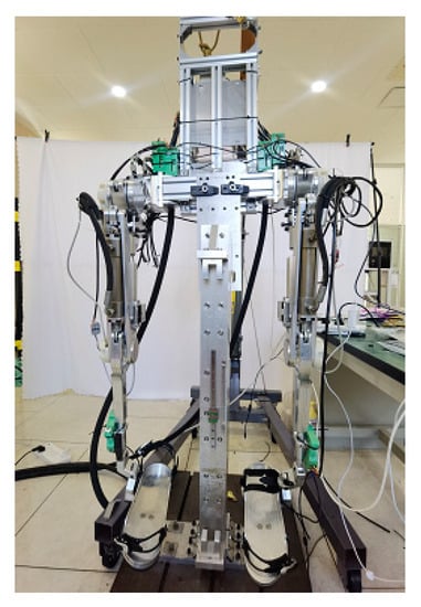
Figure 26.
Stability test.
During the 500 h test, there is no control system crash and joints out of control. All the software and hardware are working normally. The mechanical system operates smoothly. No abnormal noise, motion interference, jamming and other phenomena happen. The test results show that the exoskeleton designed in this paper has good system stability in the process of long-term continuous operation.
7.2. Load Test
The exoskeleton designed in this paper is mainly used to increase the load capacity of wearers. Therefore, the load performance of the exoskeleton is the focus of this paper. In order to verify the load performance of the exoskeleton, a load test is designed in this paper. Four wearers with a height of 1.65–1.8 m are selected. First, let the wearers walk at a speed of 0.5 m/s for 50 m along the silicone anti-skid straight road without carrying any load; then, let the wearers carry a load of 10 kg, 20 kg, 30 kg, 40 kg and 50 kg and walk at the same speed for 50 m along the silicone anti-skid straight road; finally, let the wearers wear the exoskeleton designed in this paper with 10 kg, 20 kg, 30 kg, 40 kg and 50 kg loads on the back frame, respectively. Let the wearers walk at the same speed for 50 m along the silica gel anti-skid straight road. Record the feelings of the wearers without any load. Record the feeling of walking with and without exoskeleton under the same load to finish comparative analysis. In order to ensure the safety of wearers, this paper uses a movable frame to suspend above the exoskeleton back frame. When walking, the suspension rope is in a relaxed state and does not share the load weight. If the exoskeleton breaks down accidentally or falls, the suspension rope will hang the exoskeleton to avoid injury to the wearers. The test equipment is shown in Figure 27.
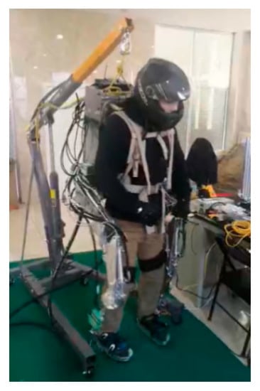
Figure 27.
Load test.
After the load test, test data is shown in Table 4.
Table 4.
Data for load test.
In Table 4, “feeling” is the subjective feeling for the wearers. Because the exoskeleton is used to increase the load capacity of the human body, compared with objective data, this paper pays more attention to the subjective feeling of the exoskeleton to wearers. Because different people have different feelings about the same assistance effect, only when the wearers subjectively feel labor saving, it can prove that the exoskeleton really has the value of practical application and promotion. Whether the test is successful or not is recorded in Table 4. Table 4 also records the wearers’ feelings about the assistance effect of the exoskeleton under different loads. All 20 groups of tests in Table 4 are successful. This also shows that the exoskeleton designed in this paper has good stability. For a 1.65 m tester, walking with the exoskeleton is close to walking without a load. It means that the exoskeleton bears the full load. For the 1.70 m and 1.75 m testers with a 10 kg load, the feeling of wearing an exoskeleton is close to that of walking without wearing an exoskeleton. Under other loads, the feeling of walking with an exoskeleton is close to that without an exoskeleton and without any load. With the increase of human height and weight, the sensitivity to power assistance decreases. For a light load, the feeling is not obvious, but when the load increases, the assistance feeling is obvious. This conclusion can also be obtained in five groups of experiments by 1.80 m testers. Based on the above analysis, it can be found that the exoskeleton designed in this paper has good loadbearing performance for a load below 50 kg. The goal of the exoskeleton in the early stage of this design is realized.
7.3. Moment following Test
The exoskeleton needs to have a good following performance with people in the process of movement, so as not to interfere with the normal walking of wearers. In order to verify the torque-following performance of the exoskeleton designed in this paper, a moment-following test is designed in this paper which is shown in Figure 28.
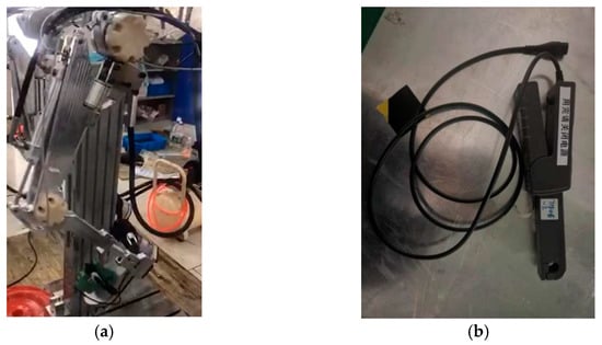
Figure 28.
Moment-following test: (a) The exoskeleton; (b) Current clamp.
In this paper, the swing phase tracking test of the exoskeleton is carried out by means of analogy input. In the test, according to the input joint angles of the CGA to the hip and knee joints, the moment calculated according to the dynamic model is the input moment. The actual output moment is calculated by the force obtained by the precision load cell. The difference between the actual moment and the calculated moment is the error which is the torque provided by the wearer.
According to CGA, in the walking process of a human being, the moment of the knee joint is approximately −10~28 and the moment of the hip joint is approximately −35~36 [20]. In Figure 29, the moment error of the knee joint is −0.5~0.5 N·m, the moment error of the knee joint is −1.6~3.2 N·m, which indicates that the moment provided by the wearer is greatly reduced.
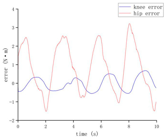
Figure 29.
Error curve for moment-following test.
7.4. Endurance Test
Endurance is another important index to evaluate the performance of the exoskeleton, so this paper designs an endurance test. Fix the waist of the exoskeleton on the fixing framework so that the exoskeleton’s feet are away from the ground. Twenty-five kg sandbags are fixed on the left foot and right foot of the exoskeleton, respectively. The total load is 50 kg. Adjust the driving speed of the hydraulic cylinder to make the exoskeleton step speed reach 1 s/step. When the battery is fully charged, start the test and move until the battery is exhausted. Repeat the experiment 20 times and record the experimental results. The test equipment is shown in Figure 30.
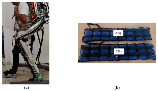
Figure 30.
Endurance test. (a) The exoskeleton; (b) Sand bag.
After 20 groups of tests, the test data are shown in Table 5.
Table 5.
Data for endurance test.
By averaging the data in Table 4, the average endurance time of 20 groups of tests is 3.34 h.
8. Conclusions
This paper analyses the action mechanism of human lower limb muscles and joints during walking. On this basis, a muscle–bone simulation model of the human lower limb is established. By the simulation, the variation laws of the lower limb joint angle and torque with time are obtained. According to the walking mechanism of the human lower limbs and joint motion angle, a design scheme of the loadbearing exoskeleton structure driven by a hydraulic system is proposed. The structure design of the parts for the exoskeleton is finished. The hydraulic control circuit is built. According to the exoskeleton structure model, a kinematic equation and dynamic equation of the loadbearing exoskeleton are established. The variation law of the exoskeleton joint torque is solved to guide the selection of a hydraulic cylinder. A finite element model of a rigid flexible coupling loadbearing exoskeleton is set up. A dynamic finite element analysis of the walking process is carried out. The location of the stress dangerous point of the parts during walking is obtained. It verifies that the parts have sufficient strength. A man–machine coupling model is established. A kinematic simulation for the walking process is conducted. The simulation result demonstrates that there is no interference between the exoskeleton and human body during the walking process. Finally, an experimental prototype is manufactured. Some performance tests are conducted. The test results indicate that the system stability of the exoskeleton is good. There is no fault during a 500 h continuous working test. The structure of the exoskeleton is simple and light, relatively. The loadbearing performance of the exoskeleton fulfils the design goal. The maximum of the load is 50 kg. The exoskeleton joints can provide sufficient torque to support a 50 kg load. The motion-following performance is good. The maximum for a delay time is less than 0.2 s. The endurance time of the exoskeleton is 3.34 h. It can fulfil the design figure. It has relatively low energy consumption.
Author Contributions
Conceptualization, Q.S.; Methodology, Q.S.; Supervision, Z.P.; Software, Z.T.; Validation, Z.T.; Formal analysis, Q.L.; Funding acquisition, Q.L.; Writing—original draft, Q.S.; Writing—review & editing, Z.P. and Z.T. All authors have read and agreed to the published version of the manuscript.
Funding
National Nature Science Foundation of China 51075017.
Institutional Review Board Statement
Not applicable.
Informed Consent Statement
Informed consent was obtained from all subjects involved in the study.
Data Availability Statement
Not applicable.
Conflicts of Interest
The authors indicated no potential conflict of interest.
References
- Hayashibara, Y.; Tanie, K.; Arai, H. Design of a power assist system with consideration of actuator’s maximum torque. In Proceedings of the 4th IEEE International Workshop on Robot and Human Communication, Tokyo, Japan, 5–7 July 1995; pp. 379–384. [Google Scholar]
- Fontana, M.; Vertechy, R.; Marcheschi, S.; Salsedo, F.; Bergamasco, M. The Body Extender: A full-body exoskeleton for the transport and handling of heavy loads. IEEE Robot. Autom. Mag. 2014, 21, 34–44. [Google Scholar] [CrossRef]
- Xi, P.Y. Mechanical Design and Simulation Analysis for a Lower Exoskeleton Robot; Tianjin University of Technology: Tianjin, China, 2021; pp. 2–10. [Google Scholar]
- Capitani, S.L.; Bianchi, M.; Secciani, N.; Pagliai, M.; Meli, E.; Ridolfi, A. Model-based mechanical design of a passive lower-limb exoskeleton for assisting workers in shotcrete projection. Meccanica 2021, 56, 195–210. [Google Scholar] [CrossRef]
- Elprama, S.A.; Vanderborght, B.; Jacobs, A. An industrial exoskeleton user acceptance framework based on a literature review of empirical studies. Appl. Ergon. 2022, 100, 103615. [Google Scholar] [CrossRef] [PubMed]
- Abhilash, C.R.; Murali, S.; Haq, M.A.; Bysani, T.N.; Narahari, N.S. Exoskeleton for lower extremities based on Indian anthropomorphism with gait allowance: Design and development. J. Eng. Des. Technol. 2021. ahead of print. [Google Scholar]
- Kim, H.K.; Hussain, M.; Park, J.; Lee, J.; Lee, J.W. Analysis of Active Back-Support Exoskeleton during Manual Load-Lifting Tasks. J. Med. Biol. Eng. 2021, 41, 704–714. [Google Scholar] [CrossRef]
- Ogunseiju, O.; Olayiwola, J.; Akanmu, A.; Olatunji, O.A. Evaluation of postural-assist exoskeleton for manual material handling. Eng. Constr. Archit. Manag. 2021. ahead of print. [Google Scholar] [CrossRef]
- Kazerooni, H.; Steger, R.; Huang, L. Hybrid Control of the Berkeley Lower Extremity Exoskeleton (BLEEX). Int. J. Robot. Res. 2006, 25, 561–573. [Google Scholar] [CrossRef]
- Zoss, A.; Kazerooni, H.; Chu, A. On the mechanical design of the Berkeley Lower Extremity Exoskeleton (BLEEX). In Proceedings of the IEEE/RSJ International Conference on Intelligent Robots and Systems, Edmonton, AB, Canada, 2–6 August 2005; pp. 3465–3472. [Google Scholar]
- Xie, H.; Li, X.; Li, W.; Li, X. The proceeding of the research on human exoskeleton. In Proceedings of the International Conference on Logistics Engineering, Management and Computer Science (LEMCS); Atlantis Press: Paris, France, 2014; pp. 752–756. [Google Scholar]
- Bogue, R. Exoskeletons and robotic prosthetics: A review of recent developments. Ind. Robot. 2009, 36, 421–427. [Google Scholar] [CrossRef]
- Young, A.J.; Ferris, D.P. State of the art and future directions for lower limb robotic exoskeletons. IEEE Trans. Neural Syst. Rehabil. Eng. 2016, 25, 171–182. [Google Scholar] [CrossRef] [PubMed]
- Karlin, S. Raiding iron man’s closet [Geek life]. IEEE Spectr. 2011, 48, 25–26. [Google Scholar] [CrossRef]
- Raut, S.; Hase, V.; Kotgire, S.; Dalvi, S.; Maske, Y. Design and Analysis of Lightweight Lower Limb Exoskeleton for Military Usage. Int. J. Res. Appl. Sci. Eng. Technol. 2021, 9, 896–907. [Google Scholar] [CrossRef]
- Murugan, B. A Review on Exoskeleton for Military Purpose. I-Manag. J. Mech. Eng. 2021, 11, 36. [Google Scholar]
- Brahmi, B.; Saad, M.; Rahman, M.H.; Ochoa-Luna, C. Cartesian trajectory tracking of a 7-DOF exoskeleton robot based on human inverse kinematics. IEEE Trans. Syst. Man Cybern. Syst. 2017, 49, 600–611. [Google Scholar] [CrossRef]
- Lan, C.W.; Lin, S.S.; Ku, C.T.; Chen, B.S.; Lo, M.F.; Chien, M.C. Using Biped Robot on Knee Exoskeleton for Stair Climbing Assistance Analysis. In Proceedings of the 2021 International Automatic Control Conference (CACS), Chiayi, Taiwan, 3–6 November 2021; pp. 1–6. [Google Scholar]
- Winter, D.A. Biomechanical Data Resources, Gait Data. 2006. Available online: http://www.isbweb.org/data/ (accessed on 5 May 2022).
- Kirtley, C. CGA Normative Gait Database. 2006. Available online: http://guardian.curtin.edu.au/cga/data/ (accessed on 5 May 2022).
- Wang, Y.X. Research on Modeling and Efficient Dynamic Computation of Multi-DOF Lower Extremity Exoskeleton Robot; Shandong University of Science and Technology: Qingdao, China, 2020; pp. 55–62. [Google Scholar]
- GB 10000-88; Human Dimensions of Chinese Adults. China Institute of Standardization and Information Classification and Coding; Standards Press of China: Beijing, China, 1988.
Publisher’s Note: MDPI stays neutral with regard to jurisdictional claims in published maps and institutional affiliations. |
© 2022 by the authors. Licensee MDPI, Basel, Switzerland. This article is an open access article distributed under the terms and conditions of the Creative Commons Attribution (CC BY) license (https://creativecommons.org/licenses/by/4.0/).