Article

Path Tracking Control of Autonomous Vehicle Based on Nonlinear Tire Model

1
College of Energy and Power Engineering, Nanjing University of Aeronautics and Astronautics, Nanjing 210016, China
2
School of Mechanical and Automotive Engineering, Liaocheng University, Liaocheng 252000, China
*
Authors to whom correspondence should be addressed.
Actuators 2021, 10(9), 242; https://doi.org/10.3390/act10090242
Submission received: 1 August 2021 / Revised: 12 September 2021 / Accepted: 13 September 2021 / Published: 21 September 2021

Abstract

:
The tire forces of vehicles will fall into the non-linear region under extreme handling conditions, which cause poor path tracking performance. In this paper, a model predictive controller based on a nonlinear tire model is designed. The tire forces are characterized with nonlinear composite functions of the magic formula instead of a simple linear relation model. Taylor expansion is used to linearize the controller, the first-order difference quotient method is used for discretization, and the partial derivative of the composite function is used for matrix transformation. Constant velocity and variable velocity conditions are selected to compare the designed controller with the conventional controller in Carsim/Simulink. The results show that when the tire forces fall in the nonlinear region, two controllers have good stability, and the tracking accuracy of the controller designed in this paper is slightly better. However, after the tire forces become nonlinear, the controller with linear tire force becomes worse, the tracking accuracy is far worse than the controller with the nonlinear tire model, and the vehicle stability is also degraded. In addition, an active steering test platform based on LabVIEW-RT is established, and hardware-in-the-loop tests are carried out. The effectiveness of the designed controller is verified.

1. Introduction

Autonomous vehicles are the focus of attention in the world today. Many car manufacturers and even some Internet companies have invested a lot of energy in the research and development of autonomous vehicles. As early as 2008, Urmson C believed that intelligent systems could be applied to the automotive industry. He introduced the advantages of autonomous vehicles and the challenges faced by cities in the direction of autonomous driving [1]. Then, Lee J analyzed the needs of autonomous vehicles, designed an agent that can simulate autonomous vehicles, and developed a prototype for it [2]. Obinata G believed that it is necessary to solve the problems of machine control, road safety and automation technology reliability of autonomous vehicles, and explained the current situation and challenges of unmanned operation technology [3]. More and more researchers are advancing the development of autonomous cars from different angles and within different fields. From the perspective of data storage, Yeshodara NS proposed a new idea to reduce the data storage problems of autonomous vehicles, only relying on cloud infrastructure to drive cars [4]. From the perspective of obstacle recognition, Hane C proposed a method of extracting static obstacles from depth maps calculated from multiple consecutive images [5]. Kumar GA proposed a method to estimate the distance between autonomous vehicles and other vehicles, objects and signs using precise fusion methods [6]. From the perspective of computer vision perception, Dongpu Cao used a direct perception method to train a deep neural network in terms of increasing learning ability in relation to autonomous driving [7]. From the perspective of path planning, Li CC proposed a model-based dynamic environment path planning algorithm [8], and Jinkai Y proposed a hybrid path planning algorithm based on a simulated annealing algorithm and a particle swarm algorithm [9]. Different research angles have brought hope to the real realization of autonomous cars to some extent; however, they must be implemented with consideration of the control of the vehicle, so path tracking control will eventually grow in importance.
In the control of autonomous cars, Jain AK installed a Raspberry Pi and cameras on the top of the car. An image was sent to the convolutional neural network for manipulation prediction, and then the prediction signal was sent to the controller to make the vehicle move in the intended direction without human intervention [10]. Chen H proposed a new path-following control method and designed a three-step controller with output feedback to realize the coordinated control of the lateral and longitudinal directions without measuring the lateral speed [11]. Li L proposed a high-performance automatic steering control strategy, using the system state equation of direction angle and lateral offset deviation to describe the tracking accuracy, and the control method adopted the sliding mode variable structure control method [12]. Zhang H proposed the use of the Takagi–Sugeno model to deal with the time-varying characteristics of vehicle speed, as well as the use of Lyapunov stability parameters to improve the transient stability of the vehicle system [13]. Celentano L proposed a simple and robust smooth path tracking control method that allows unmanned electric vehicles to track a smooth reference signal [14]. Hain H proposed the use of a fuzzy controller to collect driver data while controlling an off-road vehicle. The data were used to develop the membership function of the input and output of the fuzzy controller, thereby improving the autonomous vehicle’s path tracking ability [15]. Taking into account the conflict between tracking accuracy and stability under extreme conditions, Liang YX proposed a new path tracking controller based on yaw rate tracking [16]. Hang P proposed a control algorithm to establish a linear parameter change system model to achieve different longitudinal speeds and different road friction coefficients, and combined the use of feedforward control with linear quadratic regulators to increase tracking stability [17]. There are various vehicle motion control methods, but they are all aimed at improving control accuracy and stability. Among these control methods, model predictive control takes place earlier, and it uses non-minimized description models to improve the robustness of the system. It uses a rolling optimization strategy to make up for the uncertainty and has better dynamic performance [18], and the algorithm has the ability to deal with constraints systematically, so it is widely used to solve the path tracking problems of autonomous vehicles.
Falcone P first proposed a new automatic steering system method [19]. The designed model predictive controller emphasizes the trade-off between vehicle speed and required road preview to stabilize the vehicle. Then, Falcone P performed continuous online linearization of the complex nonlinear vehicle dynamics model [20], and also proposed a low-complexity linear time-varying model, which considers the state of the vehicle and input constraints to improve vehicle stability on slippery roads and at high speeds, and used a variety of optimization algorithms to extend the range of conditions for real-time MPC implementation. According to the literature [19,20], Falcone proposed a predictive model for the joint control of braking and steering of autonomous vehicles. On high-speed snow-covered roads, the vehicle can be better controlled to change lanes on two lanes [21]. For the problem of model mismatch caused by different road conditions and small angles of vehicle models, Guo HY adopted the form of measurable disturbance, and used differential evolution algorithm for the optimization problem of path tracker [22]. Yin GD designed a decentralized MPC controller, which considers the rear-end collision avoidance of the control area and the collision avoidance at intersections to improve traffic efficiency and safety [23]. He ZW proposed a two-layer controller for accurate and robust lateral path tracking control of highly automated vehicles. The upper controller is realized by assuming linear time-varying MPC at the small angle, and the slip angle is limited to ensure stability. The lower controller is a radial basis function neural network PID controller [24]. Peng HN proposed a robust model predictive control method with a finite time domain to realize the path tracking and direct yaw moment control of an electric vehicle independently driven by an autonomous four-wheel motor [25]. Based on the analysis of the sideslip angle, Tang LQ proposed a vehicle sideslip angle compensator that can correct the motion model prediction, which significantly improves the path tracking performance and the control ability at high speed [26]. Xu SB proposed the preview steering control algorithm and the concept of its closed-loop system analysis, and compared the model method with the MPC model based on the bicycle model [27]. Yao proposed an MPC model with longitudinal velocity compensation in the prediction range, and analyzed the longitudinal velocity change mechanism and the stability within the prediction range [28]. Sara M introduced a Tube-based MPC to consider the dynamic difference between the real vehicle and this constant nominal model, not only considering the lateral error, but also the directional error [29]. Michael J extended constraint removal to Tube-based MPC, detecting inactive constraints in advance, deleting invalid constraints, and reducing calculation time [30]. Shilp D used a combination of potential fields such as vehicle functions and reachability sets to identify safe zones on the road, and provided them to the Tube-based MPC, which can be free from non-convex collision avoidance constraints and ensure the feasibility of lateral movement during acceleration and deceleration [31]. Among the above MPC controller design processes, most chose the bicycle model to simplify the calculation of the algorithm, and used the small angle assumption to represent the tire force in the vehicle model. When the tire force enters the nonlinear region, errors will inevitably occur, which will affect the performance of the controller. Therefore, an MPC algorithm based on a nonlinear tire model is proposed: Replace the conventional tire force linearly expressed by cornering stiffness with the tire force expressed by the magic formula composite function, so that even if the tire force enters the nonlinear region, the tire force calculated by the magic formula is close to the tire force under real conditions. Avoid unnecessary errors caused by tire force in path tracking.
The main arrangement of this work is as follows. First, in the first section, a bicycle model and a non-linear magic formula tire model are established. In the second section, the complex partial derivative processing and matrix transformation related to the nonlinear tire model, as well as the prediction model, objective function and constraint conditions of the controller are introduced in detail. In the third section, a variety of constant working conditions and variable working conditions are selected, and the effectiveness of the controller is verified based on Carsim/Simulink simulation. In the fourth section, an active steering test platform based on LabVIEW-RT is established, and hardware-in-the-loop testing is carried out to verify the actual control effect of the controller. The fifth section describes the conclusion.
Only the replacement of the linearly expressed tire force with the tire force expressed by a composite function is considered to verify the performance of the controller, so as to promote the improvement and research of the controller on this basis in the future.

2. Vehicle Dynamics Model

2.1. Bicycle Model

Establishing a suitable vehicle model is the prerequisite and basis for realizing model predictive control. Since the main research goal is to make the car follow the desired path quickly and stably, the vehicle model needs to be simplified to a certain extent, and the bicycle model is used to transfer left and right without load, assuming that the vehicle has a good anti-lock braking system.
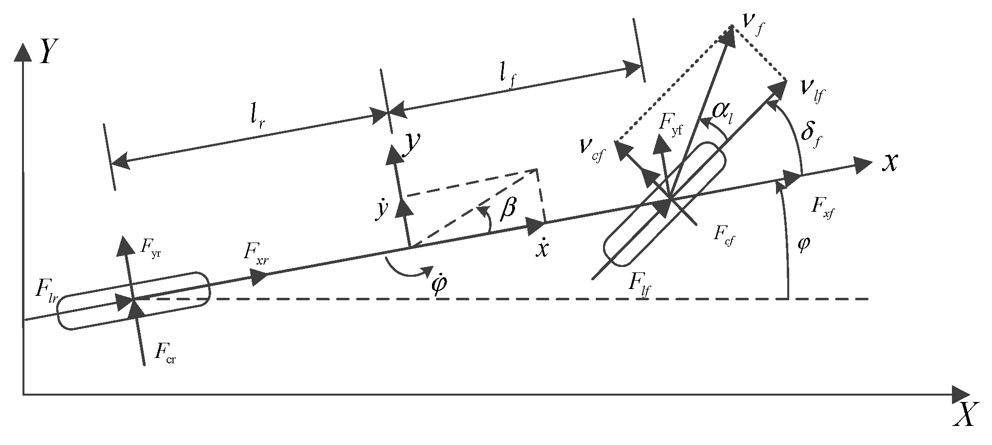
The plane motion of the vehicle is mainly considered as lateral, longitudinal and yaw motion. The vehicle is set as front-wheel drive and front-wheel steering, and the vehicle model is selected as a three-degree-of-freedom bicycle model [32]. In the plane rectangular coordinate system, the vehicle model is shown in Figure 1.
According to Newton’s second law, the force balance equations along the x-axis, y-axis and z-axis can be obtained.
In the x-axis direction:
m x ¨ = 2 F x f + 2 F x r + m y ˙ φ ˙
In the y-axis direction:
m y ¨ = 2 F y f + 2 F y r m x ˙ φ ˙
Around the z axis:
I z φ ¨ = 2 F y f l f 2 F y r l r
where m is the curb weight of the vehicle, x ˙ and y ˙ are the longitudinal and lateral speeds, F x f and F y f are the forces in the x and y directions received by the front tires, F x r and F y r are the forces in the x and y directions received by the rear tires, φ ˙ is the yaw rate, I z is the moment of inertia of the vehicle around the z-axis, and l f and l r are the distances from the center of mass to the front and rear axles.
The force received by the front and rear tires in the x and y directions is related to the longitudinal force and lateral force received by the front and rear tires. The relationship is as follows [32]:
F x f = F l f cos δ f F c f sin δ f F x r = F l r cos δ r F c r sin δ r F y f = F l f sin δ f + F c f cos δ f F y r = F l r sin δ r + F c r cos δ r
In the formula, F l f and F l r are the longitudinal forces received by the front and rear wheels, F c f and F c r are the lateral forces received by the front and rear wheels, δ f and δ r are the front and rear steering angles. Since the selected vehicle model is front-wheel steering, δ r = 0 .
The longitudinal force and lateral force of the tire can be expressed as a complex function of the tire side slip angle α , tire slip rate s , vertical load F z and other parameters:
F l = f l ( α , s , F z ) F c = f c ( α , s , F z )
Among them, the side slip angle of the tire is related to the longitudinal speed and the lateral speed, as shown in Equation (6) [32]:
α f = arctan ν c f ν l f α r = arctan ν c r ν l r
In the formula, α f and α r are the front wheel slip angle and the rear wheel slip angle, ν l f and ν l r are the longitudinal speeds of the front and rear wheels, and ν c f and ν c r are the lateral speeds of the front and rear wheels.
The longitudinal and lateral speed of each tire can be represented by the speed in the x direction, the speed in the y direction, and the front and rear steering angles [33]:
ν l f = ν y f sin δ f + v x f cos δ f ν l r = ν y r sin δ r + v x r cos δ r ν c f = ν y f cos δ f v x f sin δ f ν c r = ν y r cos δ r v x r sin δ r
In the formula, ν x f and ν x r are the speeds of the front and rear wheels in the x direction, and ν y f and ν y r are the speeds of the front and rear wheels in the y direction.
The speed of the tires in the x and y directions is generally difficult to obtain, and can be calculated from the vehicle speed [33]:
ν y f = y ˙ + l f φ ˙ ν y r = y ˙ l r φ ˙ ν x f = x ˙ ν x r = x ˙
Therefore, the front and rear wheel slip angles can be obtained from Equations (7) and (8).
Assuming that the vehicle has a good anti-lock braking system, the adhesion coefficient reaches the maximum when the tire slip rate s is 15–20%. In order to achieve the best braking effect, the slip rate needs to be controlled at 15–20% Therefore, the slip rate is a constant value of 20%.
Since the load transfer of the vehicle is not considered, assuming that the vehicle speed changes slowly and there is no load transfer of the front and rear axles, the vertical loads F z f and F z r of the front and rear wheels can be expressed as [33]:
F z f = l r m g 2 ( l f + l r ) F z r = l f m g 2 ( l f + l r )
The above formulas are derived from the body coordinate system, and the relationship conversion between the body coordinate system and the inertial coordinate system needs to be considered [33]:
Y ˙ = x ˙ sin φ + y ˙ cos φ X ˙ = x ˙ cos φ y ˙ sin φ
In the formula, φ is the yaw angle, X is the longitudinal position in the inertial coordinate system, and Y is the horizontal position in the inertial coordinate system.

2.2. Magic Formula Tire Model

In order to reduce the amount of calculation in most of the current path tracking algorithm models, the small angle assumption is used in Equation (5) to approximate the longitudinal force and lateral force of the tire. When the tire slip angle and longitudinal slip rate are small, the tire force can be linearly approximated as:
F l = C l s , F c = C c α
In the formula, C l is the tire longitudinal stiffness, and C c is the tire cornering stiffness.
The use of Equation (11) has a certain limit range, and only when the lateral acceleration a y 
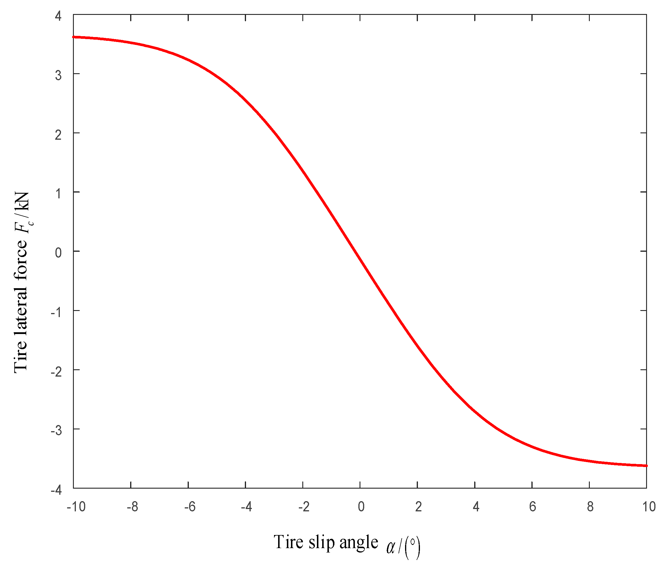
is less than 0.4 g can it have a higher fitting accuracy for conventional tires. If you consider that at a high speed or when the road adhesion coefficient is low, when the lateral acceleration of the vehicle is greater than 0.4 g at a certain moment, the tire longitudinal force and lateral force at that moment are substituted into the control algorithm model, and there will be a certain error in the calculation result. Because the increase in tire force at this time becomes slower with the increase in slip rate and cornering angle, the tire force calculated with the small-angle linear assumption is obviously greater than the tire force under real conditions. In order to make the model more accurate, the path tracking algorithm model is based on the magic formula tire model [34], replacing the small angle hypothesis of Equation (11) with the magic formula.
When the vehicle is running, the camber angle is generally small. The influence of the camber angle on the tire longitudinal force can be ignored, and the empirical parameters related to the camber in the magic formula can be ignored. Ignore the parameters related to zero-point drift, ignore the empirical parameters that cause asymmetry in the formula, and ignore the higher-order terms more than 3 times; thus, the simplified magic formula is as follows:
In the purely longitudinal case, the longitudinal force is [34]:
F x 0 = D x sin [ C x arctan { B x s x E x ( B x s x arctan ( B x s x ) ) } ] + S v x
In the formula:
s x = s + S H x , S H x = P H x 1 + P H x 2 d f z , C x = P C x 1 , D x = ( P D x 1 + P D x 2 d f z ) F z , E x = P E x 1 + P E x 2 d f z + P E x 3 d f z 2 , S v x = F z ( P V x 1 + P V x 2 d f z ) , d f z = F Z F Z 0 F Z 0 , B x = ( P K x 1 + P K x 2 d f z ) e P K x 3 d f z / [ P C x 1 ( P D x 1 + P D x 2 d f z ) ] .
In the case of pure sideslip, the lateral force is [34]:
F y 0 = D y sin [ C y arctan { B y α y E y ( B y α y arctan ( B y α y ) ) } ] + S v y
In the formula:
α y = α + S H y , S H y = P H y 1 + P H y 2 d f z , C y = P C y 1 , D y = ( P D y 1 + P D y 2 d f z ) / ( 1 + P D y 3 γ * ) F z , γ * 1 ° , E y = P E y 1 + P E y 2 d f z , S v y = F z ( P V y 1 + P V y 2 d f z ) , d f z = F Z F Z 0 F Z 0 , B y = P K y 1 F z 0 sin [ 2 arctan ( F z P K y 2 F z 0 ) ] / [ P C y 1 ( P D y 1 + P D y 2 d f z ) F z ] .
In the mixed case of longitudinal sideslip [34]:
The longitudinal force is:
F x = G x α F x 0
G x α = cos [ C x α arctan { B x α α s E x α ( B x α α s arctan ( B x α α s ) ) } ] cos [ C x α arctan { B x α S H x α E x α ( B x α S H x α arctan ( B x α S H x α ) ) } ]
In the formula:
C x α = r C x 1 , E x α = r E x 1 + r E x 2 d f z , α s = α + S H x α , S H x α = r H x 1 , B x α = r B x 1 cos ( arctan ( r B x 2 s ) ) .
The lateral force is:
F y = G y s F y 0 + S v y s
G y s = cos [ C y s arctan { B y s s s E y s ( B y s s s arctan ( B y s s s ) ) } ] cos [ C x α arctan { B y s S H y s E x α ( B y s S H y s arctan ( B y s S H y s ) ) } ]
In the formula:
s s = s + S H y s , S H y s = r H y 1 + r H y 2 d f z , C y s = r C y 1 , E y s = r E y 1 + r E y 2 d f z , B y s = r B y 1 cos ( arctan { r B y 2 ( α r B y 3 ) } ) , S v y s = μ y F z ( r v y 1 + r v y 2 d f z ) cos [ arctan ( r v y 4 α ) ] sin [ r v y 5 arctan ( r v y 6 s ) ] , μ y = ( P D y 1 + P D y 2 d f z ) / ( 1 + P D y 3 r * 2 ) ,   r * 1 ° .
Combining Equations (12)–(17) with the parameters in Table 1, the longitudinal force and lateral force of the front and rear wheels can be calculated. Equation (5) can be expressed as follows:
F l f = 4724 cos [ 1.125 arctan { 4.47 ( α f 0.03 ) 0.0015 ( 4.47 ( α f 0.03 ) arctan ( 4.47 ( α f 0.03 ) ) ) } ] F l r = 4018 cos [ 1.125 arctan { 4.47 ( α r 0.03 ) 0.0007 ( 4.47 ( α r 0.03 ) arctan ( 4.47 ( α r 0.03 ) ) ) } ] F c f = cos [ 1.1 arctan { 0.2036 B y s 1 0.2792 ( 0.2036 B y s 1 arctan ( 0.2036 B y s 1 ) ) } ] cos [ 1.1 arctan { 0.0036 B y s 1 0.2792 ( 0.0036 B y s 1 arctan ( 0.0036 B y s 1 ) ) } ] F y o f F c r = cos [ 1.1 arctan { 0.1993 B y s 2 0.2054 ( 0.1993 B y s 2 arctan ( 0.1993 B y s 2 ) ) } ] cos [ 1.1 arctan { 0.00074 B y s 2 0.2054 ( 0.00074 B y s 2 arctan ( 0.00074 B y s 2 ) ) } ] F y o r
In the formula:
B y s 1 = 6.38 cos [ arctan { 7.95 ( α f + 0.06 ) } ] , B y s 2 = 6.38 cos [ arctan { 7.95 ( α r + 0.06 ) } ] , F y o f = 4037 sin [ 1.29 arctan { 9.33 ( α f + 0.00314 ) + 0.988 ( 9.33 ( α f + 0.00314 ) arctan ( 9.33 ( α f + 0.00314 ) ) ) } ] + 190 , F y o r = 3513 sin [ 1.29 arctan { 9.87 ( α r + 0.00368 ) + 1.111 ( 9.87 ( α r + 0.00368 ) arctan ( 9.87 ( α r + 0.00368 ) ) ) } ] + 180
It can be seen from Equation (18) that the longitudinal force and lateral force of front and rear tires are only related to their respective slip angles. By substituting the above equation into Equation (4), the forces received by the front and rear tires in the x direction and the y direction are:
F x f = F l f cos δ f F c f sin δ f F x r = F l r F y f = F l f sin δ f + F c f cos δ f F y r = F c r
Substituting Equation (19) into Equations (1)–(3), and combining Equation (10), we can obtain the vehicle dynamics nonlinear model based on the magic formula tire model:
{ m y ¨ = m x ˙ φ ˙ + 2 F l f sin δ f + 2 F c f cos δ f + 2 F c r m x ¨ = m y ˙ φ ˙ + 2 F l f cos δ f 2 F c f sin δ f + 2 F l r φ ˙ = φ ˙ I z φ ¨ = 2 l f F l f sin δ f + 2 l f F c f cos δ f 2 l r F c r Y ˙ = x ˙ sin φ + y ˙ cos φ X ˙ = x ˙ cos φ y ˙ sin φ
The selected tire type is 175/70 R13 (asymmetric). The specific parameters of the tire based on the magic formula are as follows:
Table 1. 175/70 R13 (asymmetric) tire parameters.
Parameter NameParameter ValueParameter NameParameter Value
P C x 1 1.62 P C y 1 1.29
P D x 1 1.035 P D y 1 −0.9
P D x 2 −0.0487 P D y 2 0.18
P E x 1 0.5 P D y 3 −4.5
P E x 2 −0.122 P E y 1 −1.07
P E x 3 −0.0063 P E y 2 0.68
P K x 1 19.4 P K y 1 −12.95
P K x 2 −0.13 P K y 2 1.72
P K x 3 0.171 P H y 1 0.0035
P H x 1 −0.0005 P H y 2 −0.003
P H x 2 8.42 × 10⁻⁵ P V y 1 0.0045
P V x 1 0 P V y 2 −0.03
P V x 2 0 F z 0 4100
r C x 1 1.125 r C y 1 1.1
r E x 1 0.078 r E y 1 0.23
r E x 2 −0.16 r E y 2 0.41
r H x 1 −0.03 r B y 1 6.38
r B x 1 9 r B y 2 7.95
r B x 2 −8.75 r B y 3 −0.06
r H y 1 0.0007 r V y 4 10
r H y 2 0.024 r V y 5 1.95
r V y 1 0 r V y 6 −50
r V y 2 0

3. Model Predictive Controller Design

3.1. Prediction Model

Convert Equation (20) in vehicle dynamics model into state space form [33]. Select lateral velocity y ˙ , longitudinal velocity x ˙ , yaw angle φ , yaw rate φ ˙ , lateral offset Y , and longitudinal position X as the state variable x = [ y ˙ , x ˙ , φ , φ ˙ , Y , X ] T . In Equation (20), F l f , F c f , F l r , F c r are related to α f , α r , and α f , α r are related to the front steering angle δ f from Equations (6)–(8). Therefore, in the control system, the control variable is selected as u = δ f . The general form of the state equation is as follows:
x ˙ = f ( x , u )
The general vehicle path tracking control will give a reference path to realize the control tracking of the actual vehicle. The state variable and control variable of the reference vehicle at each time satisfy the above equation, and d represents the reference variable, so the form becomes:
x ˙ d = f ( x d , u d )
In the formula: x d = [ y ˙ d , x ˙ d , φ d , φ ˙ d , Y d , X d ] T , u d = δ f d .
Perform a Taylor expansion of Equation (21) at any reference trajectory point, ignoring higher-order terms, and obtain [33]:
x ˙ = f ( x d , u d ) + f ( x , u ) x | x = x d u = u d ( x x d ) + f ( x , u ) u | x = x d u = u d ( u u d )
Subtract Equations (22) and (23) to obtain:
x ˜ ˙ = A x ˜ + B u ˜
In the formula, the A matrix is the first order partial derivative matrix of f to x , and the B matrix is the first order partial derivative matrix of f to u . x ˜ = x x d , u ˜ = u u d .
Equation (24) is the state equation, but the state equation is continuous. The model predictive controller is a discrete-time control method, so Equation (24) needs to be discretized [33]:
A ( k ) = I + T A B ( k ) = T B
In the formula, T is the sampling time, and I is the 6 × 6 unit matrix.
The new discretized state space model is [33]:
x ˜ ( k + 1 ) = A ( k ) x ˜ ( k ) + B ( k ) u ˜ ( k )
In the formula:
A ( k ) = [ 1 + T y ¨ y ˙ T y ¨ x ˙ 0 T y ¨ φ ˙ 0 0 T x ¨ y ˙ 1 + T x ¨ x ˙ 0 T x ¨ φ ˙ 0 0 0 0 1 T 0 0 T φ ¨ y ˙ T φ ¨ x ˙ 0 1 + T φ ¨ φ ˙ 0 0 T cos φ T sin φ T ( x ˙ cos φ y ˙ sin φ ) 0 1 0 T ( sin φ ) T cos φ T ( x ˙ sin φ y ˙ cos φ ) 0 0 1 ] ,   B ( k ) = [ T y ¨ δ f T x ¨ δ f 0 T φ ¨ δ f 0 0 ] .
among them:
y ¨ y ˙ = 2 sin δ f m F l f α f α f y ˙ + 2 cos δ f m F c f α f α f y ˙ + 2 m F c r α r α r y ˙ y ¨ x ˙ = φ ˙ + 2 sin δ f m F l f α f α f x ˙ + 2 cos δ f m F c f α f α f x ˙ + 2 m F c r α r α r x ˙ y ¨ φ ˙ = x ˙ + 2 sin δ f m F l f α f α f φ ˙ + 2 cos δ f m F c f α f α f φ ˙ + 2 m F c r α r α r φ ˙ x ¨ y ˙ = φ ˙ + 2 cos δ f m F l f α f α f y ˙ 2 sin δ f m F c f α f α f y ˙ + 2 m F l r α r α r y ˙ x ¨ x ˙ = 2 cos δ f m F l f α f α f x ˙ 2 sin δ f m F c f α f α f x ˙ + 2 m F l r α r α r x ˙ x ¨ φ ˙ = y ˙ + 2 cos δ f m F l f α f α f φ ˙ 2 sin δ f m F c f α f α f φ ˙ + 2 m F l r α r α r φ ˙ φ ¨ y ˙ = 2 l f sin δ f I z F l f α f α f y ˙ + 2 l f cos δ f I z F c f α f α f y ˙ 2 l r I z F c r α r α r y ˙ φ ¨ x ˙ = 2 l f sin δ f I z F l f α f α f x ˙ + 2 l f cos δ f I z F c f α f α f x ˙ 2 l r I z F c r α r α r x ˙ φ ¨ φ ˙ = 2 l f sin δ f I z F l f α f α f φ ˙ + 2 l f cos δ f I z F c f α f α f φ ˙ 2 l r I z F c r α r α r φ ˙ y ¨ δ f = 2 sin δ f m F l f α f α f δ f + 2 F l f cos δ f m + 2 cos δ f m F c f α f α f δ f 2 F c f sin δ f m y ¨ x ˙ = 2 cos δ f m F l f α f α f δ f 2 F l f sin δ f m 2 sin δ f m F c f α f α f δ f 2 F c f cos δ f m y ¨ φ ˙ = 2 l f sin δ f I z F l f α f α f δ f + 2 l f F l f cos δ f I z + 2 l f cos δ f I z F c f α f α f δ f 2 l f F c f sin δ f I z
In the above formula, the partial derivatives of the side slip angle of the front and rear wheels α f , α r with respect to the longitudinal speed x ˙ , lateral speed y ˙ , yaw rate φ ˙ and front wheel rotation angle δ f can be obtained by calculating the partial derivatives of Equations (6)–(8).
Since the control variable is the front steering angle, in order to ensure the normal running of the vehicle and prevent sudden changes in the front steering angle, it is necessary to limit the front steering angle increment, so the control variable in Equation (26) is converted into a control increment [33]:
x ¯ ( k + 1 ) = A ˜ x ¯ ( k ) + B ˜ Δ u ˜ ( k )
In the formula: x ¯ ( k ) = [ x ˜ ( k ) u ˜ ( k - 1 ) ] , A ˜ = [ A 6 × 6 B 6 × 1 0 1 × 6 I 1 × 1 ] , B ˜ = [ B 6 × 1 I 1 × 1 ] , Δ u ˜ ( k ) = u ˜ ( k ) u ˜ ( k 1 ) .
The target path tracking needs to select the output of the state equation. The selected output is the yaw angle and the lateral offset. The former can be used to track and detect the forward direction of the vehicle, and the latter can be used to track and detect the forward position of the vehicle, and the output equation of the prediction model [33] is as follows [33]:
y ( k ) = C ˜ x ¯ ( k )
In the formula: C ˜ = [ 0 0 1 0 0 0 0 0 0 0 0 0 1 0 ] .
Combining Equations (27) and (28) as a complete prediction model, Equation (29):
{ x ¯ ( k + 1 ) = A ˜ x ¯ ( k ) + B ˜ Δ u ˜ ( k ) y ( k ) = C ˜ x ¯ ( k )

3.2. Output in the Forecast Time Domain

It is assumed that the prediction time domain is N p , the control time domain is N c , and the prediction time domain is greater than the control time domain. Based on Equation (29), it is predicted that N c control increments in the control time domain will act on the system. When time k is in the control time domain between the time domain and the prediction time domain, the input control amount of the system remains unchanged, and the control increment is 0. After derivation, the system’s predicted output expression can be obtained [33]:
y ˜ ( k ) = A ¯ ( k ) x ¯ ( k | k ) + B ¯ ( k ) Δ U ˜ ( k )
In the formula:
y ˜ ( k ) = [ y ( k + 1 | k ) y ( k + N p | k ) ] Δ U ˜ ( k ) = [ Δ u ˜ ( k | k ) Δ u ˜ ( k + N c 1 | k ) ] A ¯ ( k ) = [ C ˜ A ˜ C ˜ A ˜ N p ] B ¯ ( k ) = [ C ˜ B ˜ 0 0 0 C ˜ A ˜ N c 1 B ˜ C ˜ B ˜ C ˜ A ˜ N p 1 B ˜ C ˜ A ˜ N p N c B ˜ ]

3.3. Objective Function Design

The objective function is the performance standard of the system. To ensure that the unmanned vehicle can quickly and smoothly follow the target path and reflect its tracking ability, it is also necessary to optimize the deviation and control of the system state variable. It is necessary to ensure that the control increment in each sampling period is constrained to avoid sudden changes. Therefore, referring to the soft constraint method used in the literature [35], the selected objective function form is as follows:
J = i = 1 N p y ˜ ( k + i | k ) y r e f ( k + i | k ) Q 2 + i = 0 N c 1 Δ u ( k + i | k ) R 2 + ρ ε 2   = i = 1 N p q [ y ˜ ( k + i | k ) y r e f ( k + i | k ) ] 2   + i = 0 N c 1 r [ u ( k + i | k ) u ( k + i 1 | k ) ] 2 + ρ ε 2
In the formula, ρ is the weight coefficient, ε is the relaxation factor, and Q , R are the output weighting matrix and the control weighting matrix, respectively. The first item represents the accumulation of deviations between the output variable and the reference value of the output variable, which reflects the ability to follow the reference trajectory, and the second item is the accumulation of deviations of the control variable, which reflects the requirement for the steady change of the control variable. The third item ensures that there is a feasible optimal solution when changing in real time. y ˜ ( k + i | k ) is the predicted value of the output at time k in the future at time k + i , y r e f ( k + i | k ) is the reference value of the output at time k in the future at time k + i , and Δ u ( k + i | k ) is the future control variable sequence.
The output weighting matrix: Q = [ q q q ] ( 2 × N p ) × ( 2 × N p ) ,   q = [ q 1 q 2 ] 2 × 2 .
The control weight matrix: R = [ r r r ] N c × N c .
In order to simplify the calculation, the control increment matrix A is taken as a single design variable, so the objective function [36] after matrix transformation is as follows:
J = 1 2 ξ ( k ) T H ( k ) ξ ( k ) + f ( k ) ξ ( k ) + P ( k )
In the formula:
H ( k ) = [ 2 ( Θ ( k ) T Q Θ ( k ) + R ) 0 0 2 ρ ] ,   ξ ( k ) = [ Δ U ( k ) ε ] ,   f ( k ) = [ 2 E ( k ) T Q Θ ( k ) 0 ] , P ( k ) = E ( k ) T Q E ( k ) ,   E ( k ) = A ¯ ( k ) x ¯ ( k | k ) y r e f ( k | k ) .

3.4. Design of Constraints

The constraint conditions of model predictive control generally include control variable constraint, control increment constraint and output variable constraint. In real vehicle driving scenarios, the front steering angle has a certain range limit, so the actual situation should be considered when designing the controller, and the control variable front steering angle should be restricted. At the same time, in order to consider the stability of the vehicle, the constraint on the control increment is also indispensable, and the change range of the control increment cannot be too large. In addition, in order to avoid excessive deviation from the target path, it is necessary to refer to the target path to constrain the output yaw angle and lateral offset [36].
Impose constraints on the control amount:
U min ( k ) U ( k ) U max ( k )
In the formula, U min ( k ) is the minimum value of the control variable, and U max ( k ) is the maximum value of the control variable.
Impose constraints on the control increment:
Δ U min ( k ) Δ U ( k ) Δ U max ( k )
In the formula, Δ U min ( k ) is the minimum value of the control increment, and Δ U max ( k ) is the maximum value of the control increment.
Impose constraints on the output:
y ˜ min ( k ) y ˜ ( k ) y ˜ max ( k )
In the formula, y ˜ min ( k ) is the minimum value of the output and y ˜ max ( k ) is the maximum value of the output.

4. Simulation

In order to verify the performance of the proposed MPC controller based on the non-linear magic formula tires, a simulation test was carried out using the control function of Matlab/Simulink and Carsim’s vehicle dynamics model and vehicle operating environment platform.

4.1. Parameter Selection

Select the E-Class Sedan model in Carsim for simulation, and the main parameters are shown in Table 2.
This paper mainly focuses on the lateral force of the tire. According to Equations (16)–(18) and the data in Table 1 and Table 2, the relationship between the lateral force of the tire and the tire slip angle is shown in Figure 2.
In line with [33], in the lateral tracking ability experiment of unmanned vehicles, the front wheel of the vehicle is continuously turned from the left extreme position to the right extreme position. Record the corresponding time and position, and then you can measure the limit value and time of the front steering angle in clockwise and counterclockwise directions. Therefore, the constraint on the front steering angle and the front steering angle increment and the constraint on the output based on the double-shifting reference target path are shown in Equation (36):
10 ° δ f 10 ° 0.85 ° Δ δ f 0.85 ° 0.3 φ 0.21 3 Y 5

4.2. Constant Speed Simulation

4.2.1. Reference Path Selection

In the test of vehicle handling and stability, the double lane change is used widely [37,38], so the selected reference path equation is as follows [21]
Y ( X ) = d y 1 2 ( 1 + tan ( z 1 ) ) d y 2 2 ( 1 + tan ( z 2 ) )
In the formula:
z 1 = 2.4 25 ( X 27.19 ) 1.2 , z 2 = 2.4 21.95 ( X 56.46 ) 1.2 , d y 1 = 4.05 , d y 2 = 5.7 .
The reference path is shown in Figure 3:

4.2.2. Simulation Results of Constant Speed Conditions

The controller, designed based on the magic formula tire 175/70 R13 (asymmetric), takes into account the situation in which the tire part enters the nonlinear region. It is referred to as controller A below. In order to reflect the performance of controller A, it is compared with the conventional model predictive controller B. Controller B does not consider the tire entering the nonlinear region, and is only designed based on the simplification of the tire’s longitudinal stiffness and cornering stiffness. The stiffness parameters of the magic formula tire are: C c f = 48,400 , C c r = 44,800 , C l f = 90,800 , C l r = 76,200 .
(1)
First select a good road with a road adhesion coefficient of 0.8; the vehicle speed is 36 km/h, and the controller parameters are:
T = 0.05   s , N p = 10 , N c = 3 ,   Q = [ 2000 0 0 1000 ] ,   R = 5 × 10 5 , ρ = 1000 ,   ε = 1000 .
The simulation results are shown in Figure 4a–f, Figure 4a is the comparison chart of the tracking reference path, Figure 4b is the comparison chart of the front steering angle, Figure 4c is the comparison chart of the yaw rate, Figure 4d is the comparison chart of the side slip angle of the center of mass, Figure 4e is the comparison chart of lateral acceleration, and Figure 4f is the comparison chart of the tire lateral force.
First of all, it can be seen from Figure 4e that the lateral accelerations of controller A and controller B are both within 0.4 g when the vehicle speed is 36 km/h and the adhesion coefficient is 0.8. Furthermore, it can be seen from Figure 2 that the saturation value of the tire force is about 3.6 kN; combined with Figure 4f, it can be seen that the tire lateral force is in the linear region. At this time, it can be seen from Figure 4a that in the interval of 0–70 m, the tracking effects of controller A and controller B are similar, but in the interval of 70–120 m, it is obvious that the tracking effect of controller A is better than that of controller B. Although the tire force is in the linear region at this time, controller A can more accurately describe the tire forces, while controller B describes the simplified linear tire forces, so the accuracy of controller A is better than that of controller B. From Figure 4b–d, it can be seen that the front steering angle, yaw rate and side slip angle of controller A and controller B are relatively close, and the magnitude and shape of the change are similar. Although controller A generates two small fluctuations in the range of 6–10 s, controller A’s is smaller than controller B’s in terms of peak value. In summary, it can be seen that when the lateral acceleration is less than 0.4 g and the tire lateral force is in the linear region, the performance of the two controllers is close, and they can track the reference path well and smoothly, and the overall performance of controller A is slightly better.
(2)
Increase the vehicle speed from 36 km/h to 72 km/h, the road adhesion coefficient is still 0.8, and the parameters of the controller are:
T = 0.05   s , N p = 16 , N c = 3 ,   Q = [ 2000 0 0 1000 ] ,   R = 5 × 10 5 , ρ = 1000 ,   ε = 1000 .
The simulation results are shown in Figure 5a–f, Figure 5a is the comparison chart of the tracking reference path, Figure 5b is the comparison chart of the front steering angle, Figure 5c is the comparison chart of the yaw rate, Figure 5d is a comparison chart of the side slip angle of the center of mass, Figure 5e is the comparison chart of lateral acceleration, and Figure 5f is the comparison chart of tire lateral force.
It can be seen from Figure 5a that when the vehicle speed increases to 72 km/h, the tracking effects of controller A and controller B are similar in the 0–50 m interval. In the interval of 70–85 m, the tracking effect of controller A is not as good as that of controller B, but at 60 m, the peak of controller A is closer to the reference path, and in the interval of 85−120 m, controller A can control the vehicle to track the reference path earlier. On the whole, the tracking accuracy of controller A is better than that of controller B. From Figure 5b–d, the change amplitude and shape of the front steering angle, yaw rate and side slip angle of controller A and controller B are still similar. Combining the three figures and Figure 5a, it can be seen that the tracking accuracy of the two controllers is similar within 0–2 s, but the front steering angle, yaw rate and side slip angle of controller A are all smaller than that of controller B. In the 4–6 s interval, controller A is inferior to controller B. This is because during this period, controller A sacrifices some stability to increase the tracking accuracy and can control the vehicle closer to the reference path more quickly and effectively. It can be seen from Figure 5e that the lateral acceleration of the vehicle under the action of controller B is greater than 0.4 g for some time. In combination with Figure 5f, it can be seen that the tire lateral force has been saturated within 2~4 s, which indicates that the vehicle model has entered the nonlinear region during this period. The linear tire model of controller B cannot accurately describe the tire force, which affects the tracking accuracy and stability of the vehicle. The lateral acceleration of the vehicle in controller A is less than 0.4 g, and the tire force is still in the linear region. The tracking accuracy and vehicle stability are better than that of controller B. In summary, controller B tends to be unstable under this working condition, and controller A can still control the vehicle to track the reference path more smoothly and effectively.
(3)
The vehicle speed is maintained at 72 km/h, the road adhesion coefficient is 0.3, and the parameters of the controller are:
T = 0.05   s , N p = 24 , N c = 4 ,   Q = [ 2000 0 0 1000 ] ,   R = 5 × 10 5 , ρ = 1000 ,   ε = 1000 .
The simulation results are shown in Figure 6a–f, Figure 6a is the tracking reference path diagram of controller A and controller B. Figure 6b is a diagram of the front steering angle of controller A. Figure 6c is the yaw rate diagram of controller A. Figure 6d is a diagram of the side slip angle of the centroid of controller A. Figure 6e is the lateral acceleration diagram of controller A. Figure 6f is the tire lateral force diagram of controller A.
When the vehicle speed remains at 72 km/h and the road adhesion coefficient decreases from 0.8 to 0.3, it is clear that controller B in Figure 6a cannot keep up with the reference path, so only the performance effect of controller A needs to be analyzed.
From Figure 6e, it can be seen that, due to the reduction in the road adhesion coefficient, the peak value of the lateral acceleration of the vehicle exceeds 0.4 g. According to Figure 6f, within 2–6 s, the tire lateral force approaches and partially exceeds the saturation value, and the vehicle model enters the nonlinear region. In Figure 6b, the maximum front wheel rotation angle has reached 12 degrees. The maximum yaw rate in Figure 6c and the maximum lateral deflection angle of the center of mass in Figure 6d undergo a large increase as compared to Figure 5c,d. Driving at high speed on low-attachment roads, the stability of the car decreases, but from Figure 6a, it can be seen that the vehicle under the action of controller A can still keep up with the reference path more effectively as a whole.

4.3. Variable Speed Simulation

4.3.1. Reference Path Selection

The vehicle speed is changed from a constant speed to a variable speed, and a snake path is selected for the test. The reference path equation is as follows:
y = {                                               0                                   , 0 x 20 3 . 5 sin ( pi / 50 ( x - 20 ) , 20 < x 220                                               0                                       , 220 < x 300
The reference path diagram is as follows:

4.3.2. Simulation Results of Variable Speed Conditions

In order to investigate the robustness of the controller to the change of vehicle speed, the vehicle speed is set to increase from 36 km/h to 72 km/h within 0 to 10 s, and then maintain a constant speed of 72 km/h. In order to prevent the vehicle from losing control at high speeds, the road adhesion coefficient is set to 0.8, the reference path is the snake path in Figure 7, and the speed change is shown in Figure 8.
The parameters of the controller are as follows:
T = 0.05   s , N p = 17 , N c = 2 ,   Q = [ 10,000 0 0 2000 ] ,   R = 5 × 10 5 , ρ = 1000 ,   ε = 1000 .
The simulation results are shown in Figure 9a–e: Figure 9a is the comparison chart of the tracking reference path, Figure 9b is the comparison chart of the front steering angle, Figure 9c is the comparison chart of the yaw rate, Figure 9d is a comparison chart of the side slip angle of the center of mass, Figure 9e is the comparison chart of the lateral acceleration, and Figure 9f is the comparison chart of the tire lateral force.
It can be seen from Figure 9a that the tracking accuracy of the vehicle is better in the low speed stage of 0–80 m. As the vehicle speed increases, the tracking accuracy of controller B gradually decreases; while controller A can still maintain good tracking accuracy, several peaks of controller A are closer to the reference path, and the overall tracking effect of controller A is significantly better than that of controller B. Figure 9b–d show that at 12 s, the peak value of controller B is higher than that of controller A, indicating that controller B is inferior to controller A in controlling the vehicle stability at high speeds. At 14 s, the peak value of controller A is larger, because the control adaptability of controller A is stronger. With reference to Figure 9a, in the 200–250 m interval, the vehicle speed has reached 72 km/h at this time. Under the action of controller A, the vehicle can track the reference path more quickly and accurately. It can be seen from Figure 9e that the lateral accelerations of both controllers exceed 0.4 g at 10 s. Furthermore, it can be seen from Figure 9f that at about 10 s, part of the tire lateral force has reached the saturation value, and after 14 s, the tire lateral force of controller B has chattering. The linear calculation of the tire force of controller B is quite different from the real tire force. The accumulated error will affect the later tracking control effect. In contrast to controller A, the tire force calculation is closer to the real tire force, so it can still maintain a better tracking effect. In summary, in the variable speed condition, controller A can still maintain better tracking accuracy and vehicle stability than controller B.

5. Hardware in the Loop Experiment

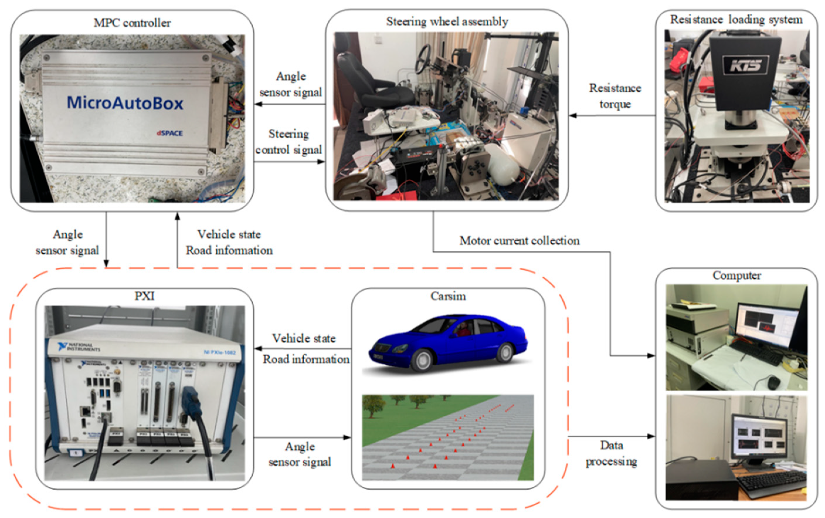
The simulation analysis in the third section preliminarily verifies the performance effect of controller A under constant speed and variable speed conditions. In order to verify the actual effect of the controller, a hardware-in-the-loop test platform based on Labview-RT is established in this section. In the hardware-in-the-loop test, although commercial simulation software is used to replace the real vehicle, the steering actuator and control system are complete physical objects. Therefore, hardware-in-the-loop testing is used by many automobile manufacturers to verify the logic of vehicle path tracking control and vehicle stability control. The test plan is shown in Figure 10 [39,40,41]. The simulation software Carsim is embedded in the automation platform PXI real-time system, and the vehicle status and road information are transmitted to the dSPACE controller through the PXI CAN card. The designed control scheme is stored in dSPACE, and the active steering angle is calculated in real time based on the vehicle status and road information transmitted by PXI. The steering signal is transmitted to the underlying controller, and the underlying controller drives the steering motor and the resistance loading system to execute the angle signal. The steering wheel is controlled to complete the angle change. The angle sensor attached to the steering wheel mechanism collects the actual steering steering angle, and then transmits the angle signal back to Carsim through the PXI CAN card. The computer collects the motor current graph and the vehicle dynamic response graph in Carsim. Through the above steps, the hardware-in-the-loop test is completed.
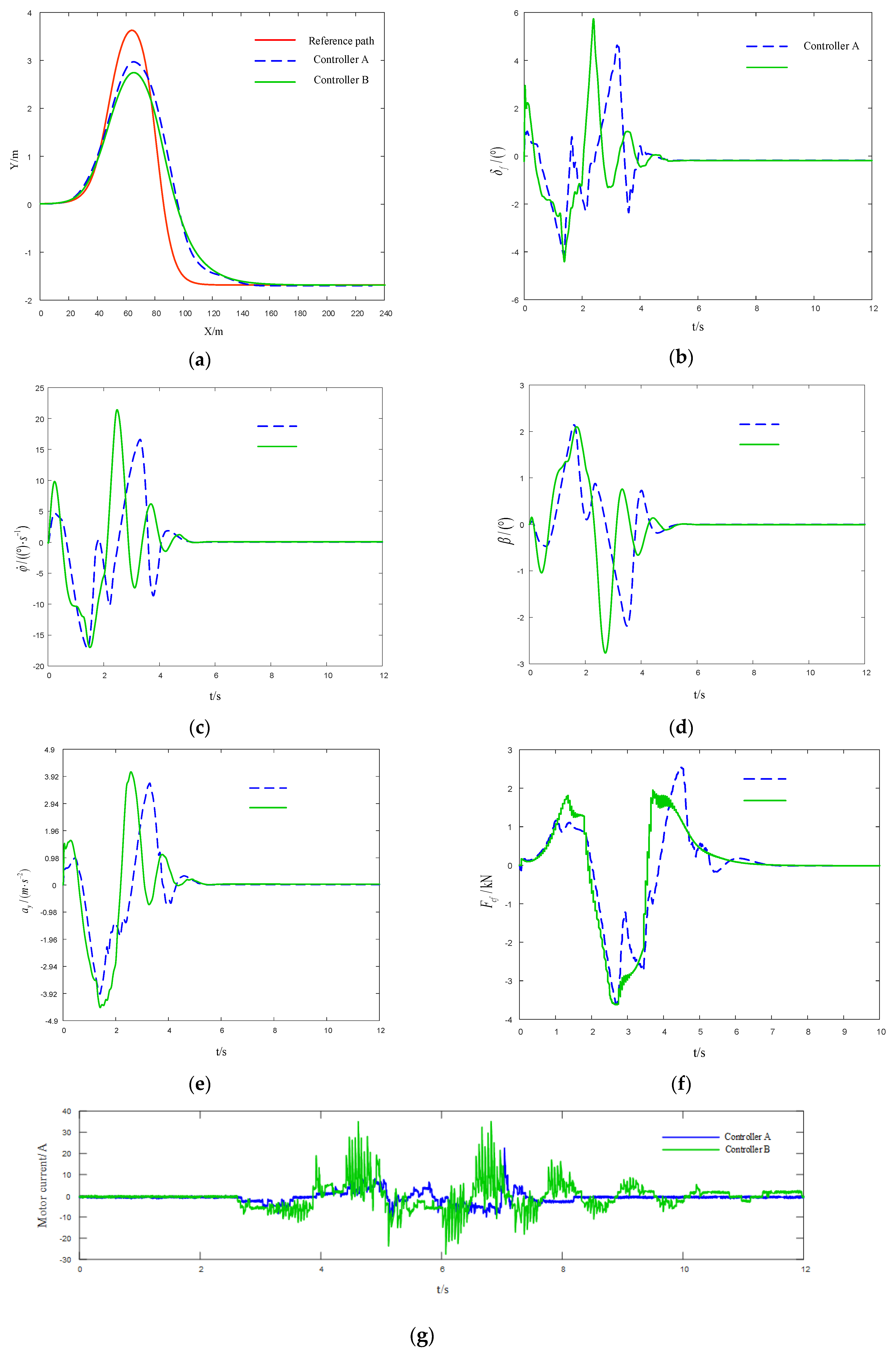
The hardware-in-the-loop test condition is selected as the constant speed condition ( μ = 0.8 ,   u = 72   km / h ) under a high adhesion coefficient, and the tracking path is still double lance change. The basic parameter settings of the controller are the same as the simulation condition. The test results are shown in Figure 11a–g; the results verify the effectiveness of the designed controller.
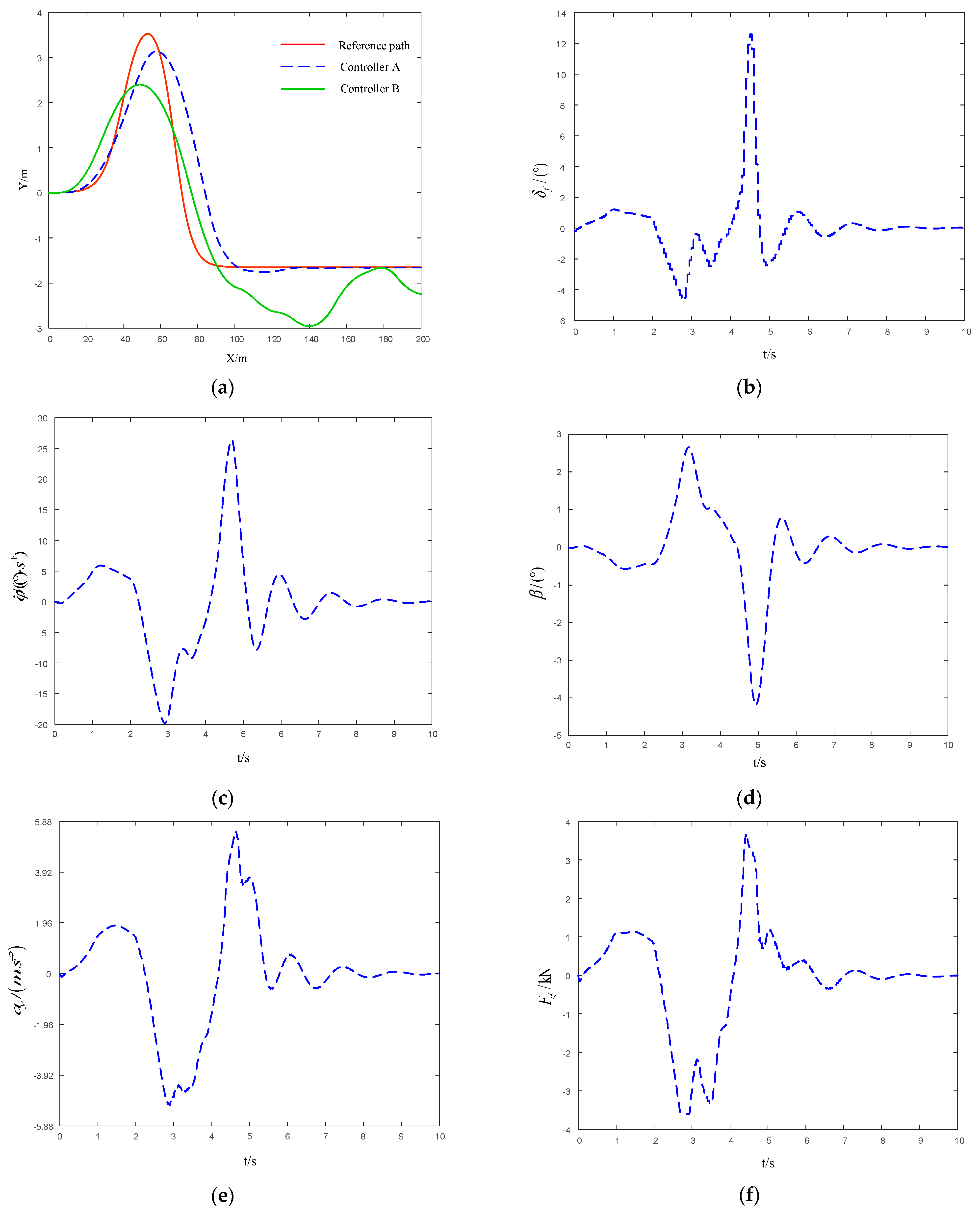
Comparing Figure 5a and Figure 11a, the path tracking effects of the two controllers in simulation and experiment are similar. Controller A is closer to the reference path at 60 m, while controller B is slightly better at 60–80 m, but controller A can keep up with the reference path more quickly and effectively after 80 m. The amplitudes and shapes of the experimental graphs 11b–d and simulation graphs 5b–d are also similar. The peak value of controller A is smaller than that of controller B. It can be seen from Figure 11e that the lateral acceleration of controller A is still within 0.4 g, while the upper and lower peaks of controller B exceed 0.4 g. Furthermore, it can be seen from Figure 11f that the tire lateral force reaches its saturation value within 2–3 s. After the tire force enters the nonlinear region, the tire force calculated by controller B has errors in terms of the real tire force, and the accumulation of errors affects the later tracking accuracy and vehicle stability.
Figure 11g is the collected motor current graph. It can be clearly seen that the current of controller B has reached ±30 A, while the current of controller A is only within ±20 A. After 8 s, the motor current of controller B is still fluctuating, while the motor current of controller A tends to be stable. The overall noise fluctuation of controller A is small, the current is more stable, and the response speed is faster. In summary, considering the path tracking accuracy and vehicle stability, the effect of controller A is better.

6. Conclusions

In this paper, a model predictive algorithm controller, based on a nonlinear tire model, is designed. It is used to reduce the calculation error of the tire force of the vehicle in the case of poor road conditions, high speed, etc., to avoid the deterioration of the path tracking effect due to excessive error. In the controller, the tire forces are characterized with nonlinear composite functions of the magic formula instead of a simple linear relation model. In the design of the controller, Taylor expansion is used for linearization, the first-order difference quotient method is used for discretization, and the partial derivative of the composite function is used for matrix transformation. Constant velocity and variable velocity conditions are selected to compare the designed controller with the conventional linear tire force controller in Carsim/Simulink. The results show that when the tire force does not fall into the nonlinear region, the stability of the two controllers is similar. The tracking accuracy of the controller designed in this paper is slightly better. However, after the tire force enters the nonlinear region, the effect of the controller, when using linear tire force, becomes worse, the tracking accuracy is far worse than the controller when using the magic formula tire design, and the vehicle stability is also degraded. In addition, a semi-physical test platform based on the LabVIEW-RT system was established, and hardware-in-the-loop test experiments were carried out. The test results verified the effectiveness of the designed controller. In order to further improve the tracking performance and stability of unmanned vehicles, the MPC model, based on nonlinear tires, that is proposed in this study will continue to be expanded in the future, so that autonomous vehicles can effectively operate in more complex and realistic traffic scenarios.

Author Contributions

Conceptualization, F.L.; methodology, F.L.; software, M.S. and C.Q.; validation, M.S. and J.W.; formal analysis, M.S. and C.Q.; investigation, F.L., M.S. and J.W.; writing—original draft preparation, M.S.; writing—review & editing, F.L. and M.S.; supervision, F.L. Project Administration, F.L.; Funding Acquisition, F.L. All authors have read and agreed to the submitted version of the manuscript.

Funding

This research was funded by the Fundamental Research Funds for the Central Universities of China, grant number NS2020016).

Acknowledgments

This work was supported by the Fundamental Research Funds for the Central Universities of China (No. NS2020016).

Conflicts of Interest

The authors declare no conflict of interest.

References

  1. Urmson, C.; Whittaker, W. Self-Driving Cars and the Urban Challenge. IEEE Intell. Syst. 2008, 23, 66–68. [Google Scholar] [CrossRef]
  2. Lee, J. Design and Prototype Development of an Agent for Self-Driving Car. J. Korea Game Soc. 2015, 15, 131–142. [Google Scholar] [CrossRef] [Green Version]
  3. Obinata, G.; Suzuki, T.; Wada, T. Tutorial I: Car Robotics—Self-Driving Cars and Human Factor. In Proceedings of the SICE 2012—51st Annual Conference of the Society of Instrument and Control Engineers of Japan, Akita, Japan, 20–23 August 2012. [Google Scholar]
  4. Yeshodara, N.S.; Kishore, N.; Namratha, S.N. Cloud Based Self Driving Cars. In Proceedings of the IEEE International Conference on Cloud Computing in Emerging Markets (CCEM), Bangalore, India, 15–17 October 2014; pp. 99–105. [Google Scholar]
  5. Hane, C.; Sattler, T.; Pollefeys, M. Obstacle Detection for Self-Driving Cars Using Only Monocular Cameras and Wheel Odometry. In Proceedings of the IEEE International Conference on Intelligent Robots and Systems, Hamburg, Germany, 28 September–2 October 2015; pp. 5101–5108. [Google Scholar]
  6. Kumar, G.A.; Lee, J.H.; Hwang, J.; Park, J.; Youn, S.H.; Kwon, S. LiDAR and Camera Fusion Approach for Object Distance Estimation in Self-Driving Vehicles. Symmetry 2020, 12, 324. [Google Scholar] [CrossRef] [Green Version]
  7. Chen, S.; Dongpu, C. Affordance Learning in Direct Perception for Autonomous Driving. arXiv 2019, arXiv:1903.08746. [Google Scholar]
  8. Li, C.C.; Wang, J.; Wang, X.N.; Zhang, Y.H. A Model based Path Planning Algorithm for Self-Driving Cars in Dynamic Environment. In Proceedings of the Chinese Automation Congress (CAC), Wuhan, China, 27–29 November 2015; pp. 1123–1128. [Google Scholar]
  9. Jinkai, Y.; Weiping, F. A Hybrid Path Planning Algorithm Based on Simulated Annealing Particle Swarm for The Self-Driving Car. In Proceedings of the International Computers, Signals and Systems Conference (ICOMSSC), Dalian, China, 28–30 September 2018; pp. 696–700. [Google Scholar]
  10. Jain, A.K. Working Model of Self-driving Car Using Convolutional Neural Network, Raspberry Pi and Arduino. In Proceedings of the 2018 Second International Conference on Electronics, Communication and Aerospace Technology (ICECA), Coimbatore, India, 29–31 March 2018; pp. 1630–1650. [Google Scholar]
  11. Wang, Y.L.; Ding, H.T.; Chen, H. Output-Feedback Triple-step Coordinated Control for Path Following of Autonomous Ground Vehicles. Mech. Syst. Signal Process. 2019, 116, 146–159. [Google Scholar] [CrossRef]
  12. Wang, P.W.; Gao, S.; Li, L. Automatic Steering Control Strategy for Unmanned Vehicles Based on Robust Backstepping Sliding Mode Control Theory. IEEE Access 2019, 7, 64984–64992. [Google Scholar] [CrossRef]
  13. Nguyen, A.T.; Sentouh, C.; Zhang, H.; Popieul, J.C. Fuzzy Static Output Feedback Control for Path Following of Autonomous Vehicles with Transient Performance Improvements. IEEE Trans. Intell. Transp. Syst. 2020, 21, 3069–3079. [Google Scholar] [CrossRef]
  14. Celentano, L.; Santini, S.; Petrillo, A. Robust Tracking Controller Design for Uncertain Nonlinear Self-Driving Cars. In Proceedings of the 18th European Control Conference (ECC), Naples, Italy, 25–28 June 2019; pp. 947–954. [Google Scholar]
  15. Halin, H.; Khairunizam, W.; Haris, H.; Razlan, Z.M.; Bakar, S.A.; Zunaidi, I.; Mustafa, W.A. Simulation Studies of the Hybrid Human-Fuzzy Controller for Path Tracking of an Autonomous Vehicle. In Proceedings of the 11th National Technical Seminar on Unmanned System Technology 2019 NUSYS’19; Springer: Berlin/Heidelberg, Germany, 2020; pp. 997–1005. [Google Scholar]
  16. Liang, Y.; Li, Y.; Zheng, L.; Yu, Y.; Ren, Y. Yaw Rate Tracking-based Path-Following Control for Four-Wheel Independent Driving and Four-Wheel Independent Steering Autonomous Vehicles Considering the Coordination with Dynamics Stability. Proc. Inst. Mech. Eng. Part D-J. Automob. Eng. 2020, 235, 260–272. [Google Scholar] [CrossRef]
  17. Hang, P.; Chen, X.B. Path Tracking Control of 4-Wheel-Steering Autonomous Ground Vehicles Based on Linear Parameter-Varying System with Experimental Verification. Proc. Inst. Mech. Eng. Part D-J. Automob. Eng. 2020, 235, 411–423. [Google Scholar] [CrossRef]
  18. Yugeng, X. Predictive Control; National Defense Industry Press: Beijing, China, 1993. [Google Scholar]
  19. Borrelli, F.; Falcone, P.; Keviczky, T.; Asgari, J.; Hrovat, D. MPC-based Approach to Active Steering for Autonomous Vehicle Systems. Int. J. Veh. Auton. Syst. 2005, 3, 265–291. [Google Scholar] [CrossRef]
  20. Falcone, P.; Borrelli, F.; Asgari, J.; Tseng, H.E.; Hrovat, D. Predictive Active Steering Control for Autonomous Vehicle Systems. IEEE Trans. Control Syst. Technol. 2007, 15, 566–580. [Google Scholar] [CrossRef]
  21. Falcone, P.; Eric Tseng, H.; Borrelli, F.; Asgari, J.; Hrovat, D. MPC-based Yaw and Lateral Stabilization Via Active Front Steering and Braking. Veh. Syst. Dyn. 2008, 46, 611–628. [Google Scholar] [CrossRef]
  22. Guo, H.; Cao, D.; Chen, H.; Sun, Z.; Hu, Y. Model Predictive Path Following Control for Autonomous Cars Considering a Measurable Disturbance: Implementation, Testing, and Verification. Mech. Syst. Signal Process. 2019, 118, 41–60. [Google Scholar] [CrossRef]
  23. Zhao, X.; Wang, J.X.; Yin, G.D. Cooperative Driving for Connected and Automated Vehicles at Non-signalized Intersection Based on Model Predictive Control. In Proceedings of the IEEE-ITSC, Auckland, New Zealand, 27–30 October 2019; pp. 2121–2126. [Google Scholar]
  24. He, Z.; Nie, L.; Yin, Z.; Huang, S. A Two-Layer Controller for Lateral Path Tracking Control of Autonomous Vehicles. Sensors 2020, 20, 3689. [Google Scholar] [CrossRef] [PubMed]
  25. Peng, H.; Wang, W.; An, Q.; Xiang, C.; Li, L. Path Tracking and Direct Yaw Moment Coordinated Control Based on Robust MPC with the Finite Time Horizon for Autonomous Independent-Drive Vehicles. IEEE Trans. Veh. Technol. 2020, 69, 6053–6066. [Google Scholar] [CrossRef]
  26. Tang, L.; Yan, F.; Zou, B.; Wang, K.; Lv, C. An Improved Kinematic Model Predictive Control for High-Speed Path Tracking of Autonomous Vehicles. IEEE Access 2020, 8, 51400–51413. [Google Scholar] [CrossRef]
  27. Xu, S.B.; Peng, H.E. Design, Analysis, and Experiments of Preview Path Tracking Control for Autonomous Vehicles. IEEE Trans. Intell. Transp. Syst. 2020, 21, 48–58. [Google Scholar] [CrossRef]
  28. Yao, Q.Q.; Tian, Y. A Model Predictive Controller with Longitudinal Speed Compensation for Autonomous Vehicle Path Tracking. Appl. Sci. 2019, 9, 4739. [Google Scholar] [CrossRef] [Green Version]
  29. Mata, S.; Zubizarreta, A.; Pinto, C. Robust Tube-Based Model Predictive Control for Lateral Path Tracking. IEEE Trans. Intell. Veh. 2019, 4, 569–577. [Google Scholar] [CrossRef]
  30. Jost, M.; Pannocchia, G.; Mönnigmann, M. Accelerating Tube-Based Model Predictive Control by Constraint removal. In Proceedings of the IEEE Conference on Decision and Control, Osaka, Japan, 15–18 December 2015; pp. 3651–3656. [Google Scholar]
  31. Dixit, S.; Montanaro, U.; Dianati, M.; Oxtoby, D.; Mizutani, T.; Mouzakitis, A.; Fallah, S. Trajectory Planning for Autonomous High-Speed Overtaking in Structured Environments Using Robust MPC. IEEE Trans. Intell. Transp. Syst. 2020, 21, 2310–2323. [Google Scholar] [CrossRef]
  32. Frendi, S.; Mellah, R.; Seddiki, L.; Akdag, H. Tracking controller design of a sideslip angle and yaw rate for electrical vehicle bicycle model. IFAC-PapersOnLine 2016, 49, 169–174. [Google Scholar] [CrossRef]
  33. Gong, J.; Jiang, Y.; Xu, W. Model Predictive Control for Self-Driving Vehicles; Beijing Institute of Technology Press: Beijing, China, 2014. [Google Scholar]
  34. Pacejka, H. Tire and Vehicle Dynamics; Butterworth Heinemann: Oxford, UK, 2012. [Google Scholar]
  35. Li, S.B.; Wang, J.Q.; Li, K.Q. Stabilization of Linear Predictive Control Systems with Softening Constraints. J. Tsinghua Univ. Sci. Technol. 2010, 50, 1848–1852. [Google Scholar]
  36. Kuhne, F.; Lages, W.F.; da Silva, J.G., Jr. Model Predictive Control of a Mobile Robot Using Linearization. In Proceedings of the Mechatronics and Robototics, Aachen, Germany, 13–15 September 2004; pp. 525–530. [Google Scholar]
  37. Zong, C.F.; Guo, K.H. Objective Evaluation Index for Handling and Stability of Vehicle. J. Nat. Sci. Jilin Univ. Technol. 2000, 30, 544–554. [Google Scholar]
  38. Xiong, L.; Yu, Z.; Jiang, W.; Jiang, Z. Research on Vehicle Stability Control of 4WD Electric Vehicle Based on Longitudinal Force Control Allocation. J. Tongji Univ. Nat. Sci. 2010, 38, 417–421. [Google Scholar]
  39. Guangtong, B.; Chunjiang, B.; Jian, W. A Robust Guiding Torque Control Method for Automatic Steering Using LMI Algorithm. IEEE Acess 2020, 8, 22162–22169. [Google Scholar]
  40. Chunjiang, B.; Jiwei, F.; Jian, W. Model Predictive Control of Steering Torque in Shared Driving of Autonomous Vehicles. Sci. Process 2020, 103, 0036850420950138. [Google Scholar]
  41. Jiwei, F.; Chunjiang, B.; Jian, W. Research on Methods of Active Steering Control Based on Receding Horizon Control. Energies 2018, 11, 2243. [Google Scholar]
Figure 1. Three-degree-of-freedom bicycle model.
Actuators 10 00242 g001
Figure 2. Tire lateral force.
Actuators 10 00242 g002
Figure 3. Reference path.
Actuators 10 00242 g003
Figure 4. (a) Comparison of tracking reference paths; (b) comparison of front steering angles; (c) comparison of yaw rates; (d) comparison of side slip angles of the centroid; (e) comparison of lateral acceleration; (f) comparison of tire lateral force.
Actuators 10 00242 g004aActuators 10 00242 g004b
Figure 5. (a) Comparison of tracking reference paths; (b) comparison of front steering angles; (c) comparison of yaw rates; (d) comparison of side slip angles of the centroid; (e) comparison of lateral acceleration; (f) comparison of tire lateral force.
Actuators 10 00242 g005aActuators 10 00242 g005b
Figure 6. (a) Comparison of tracking reference paths; (b) front steering angle diagram of Controller A; (c) the yaw rate diagram of Controller A; (d) the side slip angle diagram of Controller A; (e) lateral acceleration diagram of Controller A; (f) the tire lateral force diagram of Controller A.
Actuators 10 00242 g006
Figure 7. Reference path.
Actuators 10 00242 g007
Figure 8. Vehicle speed change graph.
Actuators 10 00242 g008
Figure 9. (a) Comparison of tracking reference paths; (b) comparison of front steering angles; (c) comparison of yaw rates; (d) comparison of side slip angles of the centroid; (e) comparison of lateral acceleration; (f) comparison of tire lateral force.
Actuators 10 00242 g009aActuators 10 00242 g009b
Figure 10. Hardware-in-the-loop test structure diagram.
Actuators 10 00242 g010
Figure 11. (a) Comparison of tracking reference paths; (b) comparison of front steering angles; (c) comparison of yaw rates; (d) comparison of side slip angles of the centroid; (e) comparison of lateral acceleration; (f) comparison of tire lateral force; (g) comparison of motor current.
Actuators 10 00242 g011
Table 2. Vehicle parameters.
Parameter NameParameter ValueParameter NameParameter Value
Vehicle quality/kg m = 1723 Distance from the center of mass of the vehicle to the front axle/m l f = 1.232
Moment of inertia around the z axis/(kg·m2) I z = 4175 Distance from the center of mass of the vehicle to the rear axle/m l r = 1.468
Vehicle wheelbase/m L = 2.7
Publisher’s Note: MDPI stays neutral with regard to jurisdictional claims in published maps and institutional affiliations.

