Pressure Estimation of the Electro-Hydraulic Brake System Based on Signal Fusion

Abstract

At present, the master cylinder pressure estimation algorithm (MCPE) of electro-hydraulic brake systems (EHB) based on vehicle dynamics has the disadvantages of poor condition adaptability, and there are delays and noise in the estimated pressure; however, the MCPE based on the characteristics of an EHB (i.e., the pressure–position relationship) is not robust enough to prevent brake pad wear. For the above reasons, neither method be applied to engineering. In this regard, this article proposes a MCPE that is based on signal fusion. First, a five-degree-of-freedom (5-DOF) vehicle model that includes longitudinal motion, lateral motion, yaw motion, and front and rear wheel rotation is established. Based on this, an algebraic expression for MCPE is derived, which extends the MCPE from a straight condition to a steering condition. Real vehicle tests show that the MCPE based on the 5-DOF vehicle model can effectively estimate the brake pressure in both straight and steering conditions. Second, the relationship between the hydraulic pressure and the rack position in the EHB is tested under different brake pad wear levels, and the results show that the pressure–position relationship will change as the brake pad is worn down, so the pressure estimated by the pressure–position model based on fixed parameters is not robust. Third, a MCPE based on the fusion the above two MCPEs through the recursive least squares algorithm (RLS) is proposed, in which the pressure-position model can be updated online by vehicle dynamics and the final estimated pressure is calculated based on the updated pressure–position model. Finally, several simulations based on vehicle test data demonstrate that the fusion-based MCPE can estimate the brake pressure accurately and smoothly with little delay and is robust enough to prevent brake pad wear. In addition, by setting the enabling conditions of RLS, the fusion-based MCPE can switch between driving and parking smoothly; thus, the fusion-based MCPE can be applied to all working conditions.

1. Introduction

Under the global trend of electrification and intelligence, automobile braking systems have undergone new changes. Traditional braking systems are increasingly unable to meet the new demands, and brake-by-wire systems (BBW) have come into existence. BBW are mainly divided into electro-mechanical brake systems (EMB) and electro-hydraulic brake systems (EHB). EMB, in which the motor drives the reduction gears to directly push the pad to clamp the disc, cancels the hydraulic components and can control the clamping force accurately and quickly. It is considered to be the supreme form of BBW; however, the braking capacity of EMB depends on a 42 V power supply system, which is not equipped on most vehicles. More importantly, the EMB does not meet the requirements of current regulations for brake system failure backup. Therefore, although some companies and universities worldwide have developed EMB prototypes [1,2,3], such as Bosch, Akipollo, Hanyang University, etc., EMB have not yet entered the market. In contrast, EHB retains the hydraulic brake circuit and adopts the motor and reduction gears to push the master cylinder piston to build pressure. It has a lower cost, and it is easier to realize failure backup. Moreover, EHB can also achieve satisfactory brake control through a suitable pressure control algorithm. In addition, since the area of the wheel cylinder piston is larger than that of the master cylinder piston, the hydraulic circuit can amplify the thrust at the master cylinder so that the 12 V on-board power supply system can meet the power requirements of the EHB. Therefore, EHB is considered to be the first approach to BBW [4]. Currently, EHB have been mass-produced, such as Bosch’s i-Booster [5] and Hitachi’s e-ACT [6].

From the perspective of vehicle dynamics, the essence of brake control is the control of the braking force. Due to the fact that it is difficult to measure the braking force acting on the wheels, EHB usually implements closed-loop pressure control by installing a pressure sensor in the master cylinder, thus indirectly controlling the braking force. As the core technology of EHB, the master cylinder pressure control algorithm (MCPC), which ensures that the EHB can realize high-performance regenerative braking control and active braking control, has been extensively studied, including aspects such as friction compensation technology [7,8,9,10], multi-closed-loop control architecture [11,12,13,14], robust control algorithms [15,16,17], etc. However, as one of the critical safety components of automobiles, once the pressure sensor fails, the function of MCPC, which is based on the pressure sensor, will be seriously affected. Some products have adopted two pressure sensors in the master cylinder for mutual inspection as a solution for failure detection and backup, which has led to a further increase in cost [18]. For this reason, master cylinder pressure estimation (MCPE) is a promising solution to the above-mentioned problems.

At present, according to different models, MCPE of EHB can be classified into three categories: (1) MCPE based on the characteristics of EHB (i.e., pressure–position relationship and EHB dynamics); (2) MCPE based on vehicle dynamics; and (3) MCPE based on intelligent algorithms.

1.1. MCPE Based on EHB’s Own Characteristics

Under braking, the master cylinder piston squeezes the brake fluid in the brake circuit to generate hydraulic pressure. During this process, the master cylinder piston position, which can be obtained from the motor rotational angle and the transmission ratio of the reduction gears, and the hydraulic pressure will form a nonlinear relationship, which is known as the so-called pressure–position relationship. In addition, the moving parts of EBH satisfy the force balance equation, namely the dynamics of the EHB, which mainly include the motor force term, the friction force term, and the hydraulic pressure term. The existing literature mainly focuses on the above two aspects to estimate the brake pressure. Refs. [9,11,14] obtained pressure–position models by polynomial fitting and by a look-up table. However, due to the hysteresis and time-varying characteristics of the pressure–position relationship, the above methods were not accurate and robust. In [19], the pressure was estimated based on EHB dynamics, and simulation results showed that drastic fluctuation occurred when the piston moved forward and back due to the no-linearity of friction. To this end, Ref. [13] proposed an interconnected pressure estimation method in which the key characteristic parameter of the pressure–position curve, namely the nonlinearly parameterized perturbations, could be estimated via EHB dynamics based on the LuGre friction model. For this method, though the pressure–position model could be updated online, the friction model, which depended on the piston position, was not robust when the pressure–position curve changes.

The MCPE of EHB is a novel topic, and there is not much research related to this topic at present; however, some of the previous research conducted on EMB can be instructive. In fact, EMB and EHB have certain similarities in the friction of the reduction gears and load characteristics (i.e., pressure–position relationship for EHB and the clamping force–motor angle relationship for EMB). In addition, limited by the cost and installation space of the clamping force sensor, EMB also needs to estimate the clamping force. Ref. [20] developed a clamping force estimation algorithm based on EMB dynamics. To avoid the need for a friction model, a high-frequency low-amplitude sinusoid was superimposed on the gross angular motion from the motor. This served to force the motor to pass the same location in a short period of time between a clamping and a releasing action. Using this method, the friction term could be cancelled out due to a sign change from clamping to releasing and vice versa, and the clamping force could be calculated. Ref. [21] obtained a first-order clamping force–motor angle model through system identification. Taking into account the time-varying characteristics of the clamping force–motor angle relationship caused by brake pad wear, when the vehicle is in a parking position, the method of [20] can be used to adapt the clamping force–motor angle model based on least squares (LS). The major issue with the method of [20,21] when applied in EHB is that the friction in EHB is not symmetrical because the friction in the pressurization process is larger than that in the depressurization process at the same location, so the friction cannot be thoroughly cancelled out [17].

It can be seen from the above references that the brake pressure can be simply and directly estimated by an EHB pressure–position model, but this method is not robust enough to prevent brake pad wear. For this reason, the pressure–position model can be updated based on EHB dynamics. However, due to the lack of a robust friction model, the MCPE based on the fusion of EHB characteristics cannot guarantee robustness either.

1.2. MCPE Based on Vehicle Dynamics

During the braking process, the hydraulic pressure pushes the pad to clamp the disc to force the vehicle to decelerate. Therefore, the longitudinal deceleration of the vehicle can reflect the pressure value to a certain extent. Ref. [22] proposed a MCPE based on vehicle longitudinal dynamics and wheel rotational dynamics for the first time. However, the brake linings’ coefficient of friction (BLCF) was regarded as constant. In fact, the BLCF is greatly affected by vehicle speed, brake pressure, and the temperature of the brake lining [23]. Ref. [24] introduced the evolution of BLCF at different initial temperatures, different initial vehicle speeds, and different brake pressures through real vehicle tests. The results show that under normal driving conditions, the evolution of BLCF is mainly related to vehicle speed; thus, a revised BLCF model is proposed. As expected, the accuracy of the estimated pressure was further improved after the adoption of the revised BLCF model. In addition, by introducing the inertial measurement unit (IMU), the MCPE based on vehicle dynamics could be extended from level roads to slope roads in [24]. Although the MCPE based on vehicle dynamics avoids the nonlinear and time-varying characteristics of EHB, it is limited by many restrictions. First, according to the principle of the algorithm, when the vehicle is stopped on a flat road, the longitudinal acceleration measured by the IMU is zero, and the MCPE based on vehicle dynamics is invalid. Second, the existing literature only studies the MCPE under straight conditions, and the research regarding braking with steering conditions, which is very common in daily driving, has not yet been conducted. Third, the estimated pressure is directly calculated based on the sensor signals and the vehicle model, and there is a lot of noise (especially when encountering bad roads and even speed bumps). Finally, the IMU is installed on the vehicle body, and it measures the motion state of the vehicle body. However, in the braking process, the hydraulic pressure first decelerates the wheel speed, and the deceleration is then transmitted to the vehicle body. That is, the signal of the IMU lags behind the hydraulic pressure, which results in the estimated pressure lagging behind the actual pressure.

1.3. MCPE Based on Intelligent Algorithms

In recent years, machine learning has increasingly been applied to the state estimation of vehicles due to the availability of large amounts of training data. The ability of machine learning to learn from data and to self-optimize behavior makes it well suited to estimate vehicle state in complex and dynamic environments [25,26]. Ref. [27] proposed a brake pressure estimation method based on a multilayer artificial neural network (ANN) with a Levenberg–Marquardt backpropagation (LMBP) training algorithm. Real vehicle tests were conducted on a chassis dynamometer under the new European driving cycle (NEDC). Experimental data for the vehicle and powertrain systems were collected to train the developed multilayer ANN. The results show that the proposed method can accurately estimate the brake pressure. However, the training method for conventional back propagation suffers from the problems of overfitting, a vanishing gradient as well as higher computational complexity in training. To this end, in [28], a deep neural network (DNN) was structured and was trained using deep-learning training techniques, such as dropout and rectified units, and a more accurate estimation was finally obtained. In [29], a time-series model based on multivariate deep recurrent neural networks (RNN) with long short-term memory (LSTM) units was developed for brake pressure estimation. This model also included a vehicle speed estimation module, which contributed to a more precise pressure estimation. Test data show that the proposed method was able to estimate the brake pressure for the next 2s in the future with a root mean square error (RMSE) of 5bar. In all of the above research, the training and model verification were conducted offline. For the possibility of being applied in real vehicles, the robustness of the algorithm needs to be further verified. In addition, only the training data include vehicle signals and powertrain signals without EHB signals and IMU signals. Therefore, the estimation model based on intelligent algorithms lacks theoretical data and persuasiveness.

As summarized by the above literature, the existing MCPEs are not able to simultaneously solve the problems of poor robustness, poor working condition adaptability, signal noise, and delay. In this regard, this paper proposes a MCPE that integrates vehicle dynamics and the pressure–position relationship. Two main contributions make this work distinctive from the previous studies: (1) a MCPE based on the five-degree-of-freedom (5-DOF) vehicle model is proposed so that the pressure can be estimated under steering conditions, and (2) a pressure estimation method realized by fusing the vehicle dynamics-based MCPE and the pressure–position-based MCPE through the recursive least squares (RLS) is proposed, in which the robustness of the pressure–position-based MCPE has been improved, and the adaptability of the working conditions of a vehicle dynamics-based MCPE has been strengthened, and the noise and delay have been reduced. The rest of this article is organized as follows: The test vehicle is introduced in Section 2. The MCPE based on a 5-DOF vehicle model is proposed and verified via a vehicle test in Section 3. The pressure–position relationship under different brake pad wear levels is tested, and a novel dynamic pressure–position model is introduced in Section 4. The MCPE based on signal fusion is proposed in Section 5 and includes the principle of the RLS with a forgetting factor, initial state setting, and update condition setting. Simulations based on experimental data are conducted to verify the proposed fusion-based MCPE in Section 6. Section 7 concludes the article.

2. Test Vehicle

The test vehicle and the in-vehicle network system have been elaborated in the author’s previous research [24], in which signals of the anti-lock brake system (ABS) (i.e., wheel speeds), electric power steering system (EPS) (i.e., wheel steering angle), IMU (i.e., absolute longitudinal acceleration, absolute lateral acceleration, and yaw rate), and EHB (i.e., rack position and master cylinder pressure) can be obtained by the EHB controller. In order to save space, this article only presents the picture and parameters of the of the test vehicle as shown in Figure 1 and

Table 1. Configuration and parameters of the test vehicle.

Item	Value
Vehicle type	SUV-class electric vehicle
Powertrain type	Front-wheel drive
Braking system type	Electro-hydraulic brake
Steering system type	Electric power steering
Vehicle mass	1580 kg
Rolling radius of all wheels	0.3183 m
Wheelbase	2.56·m
Distance between the front axle and the center of gravity	1.33·m
Distance between the rear axle and the center of gravity	1.23·m
Yaw inertia moment	2370 kg·m2
Braking force distribution coefficient	0.78

, respectively.

3. MCPE Based on 5-DOF Vehicle Model

In order to ensure safety and comfort, braking is often applied when steering in daily driving. In the literature, MCPE on flat roads [22] and sloped roads [24] without steering based on the longitudinal vehicle dynamics have been studied. In order to estimate the brake pressure under steering conditions, this article proposes an MCPE based on a 5-DOF vehicle model.

A vehicle dynamic model is usually used to describe the dynamics of vehicles. It is mainly derived through Newton’s law [30]. By considering the accuracy and complexity of the model, this article selects a 5-DOF vehicle model that includes longitudinal motion, lateral motion, yaw motion, and front and rear wheel rotation for the purposes of this research, as shown in Figure 2.

There are some assumptions of the 5-DOF vehicle model that are considered in this article.

• Ignoring the Ackerman steering principle, the left front wheel and the right front wheel share the same steering angle, that is, the vehicle is symmetrical.
• The rolling resistance and the wind resistance are very small compared to the braking force; therefore, the rolling resistance and the wind resistance are all in the longitudinal dynamics, and there is no projection in the lateral dynamics under steering conditions.
• The moment of inertia of the wheels is ignored so that the longitudinal tire force is the same as the friction braking force of each wheel.
• All of the wheels share the same rolling radius, which is a reasonable assumption for most vehicles [22,31].
• This work investigates the MCPE in ordinary braking scenarios. The ABS must not work, and all of the wheels share the same pressure.
• The master cylinder pressure is the same as that of the wheel cylinders. In other words, the throttling effect of ABS is ignored.

Based on the above assumptions, the longitudinal, lateral, and yaw dynamics of the vehicle can be derived from Equations (1)–(3), according to Newton’s law:

$$M\left({\dot{v}}_x-\omega v_y\right)=-F_{fx}\mathit{cos}\delta -F_{fy}\mathit{sin}\delta -F_{rx}-F_r-F_w,$$

(1)

$$M\left({\dot{v}}_y+\omega v_x\right)=F_{fy}\mathit{cos}\delta -F_{fx}\mathit{sin}\delta -F_{fy}\mathit{sin}\delta +F_{ry},$$

(2)

$$I\dot{\omega }=\left(F_{fy}\mathit{cos}\delta -F_{fx}\mathit{sin}\delta \right)L_f-F_{ry}{L}_r,$$

(3)

where $M$ denotes the mass of the vehicle, $kg$; $v_x$ and $v_y$ denote the longitudinal speed and the lateral speed of the vehicle, respectively, $m/s$; $\omega$ denotes the yaw rate of the vehicle, $rad/s$; $F_{fx}$ and $F_{fy}$ denote the longitudinal tire force and the lateral tire force of the front wheel, $N$; $F_{rx}$ and $F_{ry}$ denote the longitudinal tire force and the lateral tire force of the rear wheel, $N$; $\delta$ denotes the steering angle of the front wheel, $rad$; $F_r$ and $F_w$ denote the rolling resistance and the wind resistance, respectively, $N$; $I$ denotes the yaw inertia moment of the vehicle, $kg\cdot m^2$; $L_f$ denotes the distance between the front axle and the center of gravity of the vehicle, $m$; $L_r$ denotes the distance between the rear axle and the center of gravity of the vehicle, $m$.

The sum of the rolling resistance and the wind resistance (i.e., $F_r+F_w$) in Equation (1) is the so-called driving resistance, which can be obtained through the coasting test. For specific principles, the test procedures, and the test results of the coasting test, please refer to [24].

The rotational dynamics of the front wheel and the rear wheel are expressed by Equation (4) and Equation (5), respectively.

$$F_{fx}=\frac{p\left(k_{fl}+k_{fr}\right)}{r},$$

(4)

$$F_{rx}=\frac{p\left(k_{rl}+k_{rr}\right)}{r},$$

(5)

where $p$ denotes the pressure in the hydraulic circuit, $bar$; $r$ denotes the rolling radius of all wheels, $m$; $k_{fl}$, $k_{fr}$, $k_{rl}$ and $k_{rr}$, which are related to the time-varying BLCF and other time-invariant parameters of the brakes, denote the pressure–torque conversion factor of the front left wheel, front right wheel, rear left wheel, and rear right wheel, respectively, $Nm/bar$. Ref. [24] noted that under normal driving conditions, the BLCF is mainly related to the relative speed of the pad and disc, and the sum of the pressure–torque conversion factors of all of the wheels is given as Equation (6):

$$k_{fl}+k_{fr}+k_{rl}+k_{rr}=\{\begin{array}{ll}70-\frac{70-53}{25}u& ,u\le 25\\ 53& ,u>25\end{array},$$

(6)

where $u$ denotes the average wheel speed under both straight and steering conditions, $km/h$.

For most passenger cars, the ratio of the braking force between the front and rear brakes is a fixed value [32], as shown in Equation (7):

$$\frac{F_{fx}}{F_{fr}}=\frac{\frac{p\left(k_{fl}+k_{fr}\right)}{r}}{\frac{p\left(k_{rl}+k_{rr}\right)}{r}}=\frac{k_{fl}+k_{fr}}{k_{rl}+k_{rr}}=\frac{\beta }{1-\beta },$$

(7)

where $\beta =\frac{F_{fx}}{F_{fx}+F_{fr}}$ denotes the braking force distribution coefficient. Thus, $\left(k_{fl}+k_{fr}\right)$ and $\left(k_{rl}+k_{rr}\right)$ can be determined based on Equations (6) and (7).

The IMU is mounted on the vehicle body and can measure the absolute longitudinal acceleration, absolute lateral acceleration, and yaw rate of the vehicle, as shown in Equations (8)–(10):

$${\dot{v}}_x-\omega v_y=a_{x\_IMU},$$

(8)

$${\dot{v}}_y+\omega v_x=a_{y\_IMU},$$

(9)

$$\omega ={\omega }_{IMU},$$

(10)

where $a_{x\_IMU}$, $a_{y\_IMU}$, and ${\omega }_{IMU}$ denote the absolute longitudinal acceleration, absolute lateral acceleration, and yaw rate of the vehicle measured by the IMU, respectively.

Substituting Equations (4), (5) and (8)–(10) into Equations (1)–(3), we can derive Equations (11)–(13).

$$M{a}_{x\_IMU}=-\frac{p\left(k_{fl}+k_{fr}\right)}{r}\mathit{cos}\delta -F_{fy}\mathit{sin}\delta -\frac{p\left(k_{rl}+k_{rr}\right)}{r}-F_r-F_w,$$

(11)

$$M{a}_{y\_IMU}=F_{fy}\mathit{cos}\delta -\frac{p\left(k_{fl}+k_{fr}\right)}{r}\mathit{sin}\delta -F_{fy}\mathit{sin}\delta +F_{ry},$$

(12)

$$I{\dot{\omega }}_{IMU}=\left(F_{fy}\mathit{cos}\delta -\frac{p\left(k_{fl}+k_{fr}\right)}{r}\mathit{sin}\delta \right)L_f-F_{ry}{L}_r,$$

(13)

where ${\dot{\omega }}_{IMU}$ can be obtained by the difference of ${\omega }_{IMU}$. Note that Equations (11)–(13) are linear and unrelated to the three unknown variables (i.e., $p$, $F_{fy}$, and $F_{ry}$), so there is a unique solution to the equation set consisting of Equations (11)–(13). The algebraic expression of the pressure estimation algorithm based on the 5-DOF vehicle model can be derived by solving the above-mentioned equation set.

$$p=\frac{\left(-M{a}_{x\_IMU}-F_r-F_w\right)L\mathit{cos}\delta -M{a}_{y\_IMU}{L}_r\mathit{sin}\delta -I{\dot{\omega }}_{IMU}\mathit{sin}\delta }{\left(k_{fl}+k_{fr}\right)L+\left(k_{rl}+k_{rr}\right)L\mathit{cos}\delta }r,$$

(14)

where $L=L_f+L_r$ denotes the wheelbase of the vehicle. If $\delta =0$, Equation (14) degenerates to Equation (15), as in Ref [24].

$$p=\frac{-M{a}_{x\_IMU}-F_r-F_w}{k_{fl}+k_{fr}+k_{rl}+k_{rr}}r,$$

(15)

From Equations (14) and (15), we can see that with input signals of sensors (i.e., IMU and wheel steering angle), vehicle parameters (i.e., $M$, $L$ and, etc.), driving resistance and pressure-torque conversion factors, the brake pressure can be estimated online. Besides, Equation (14) is applicable to both straight and steering condition while Equation (15) is only applicable to straight condition.

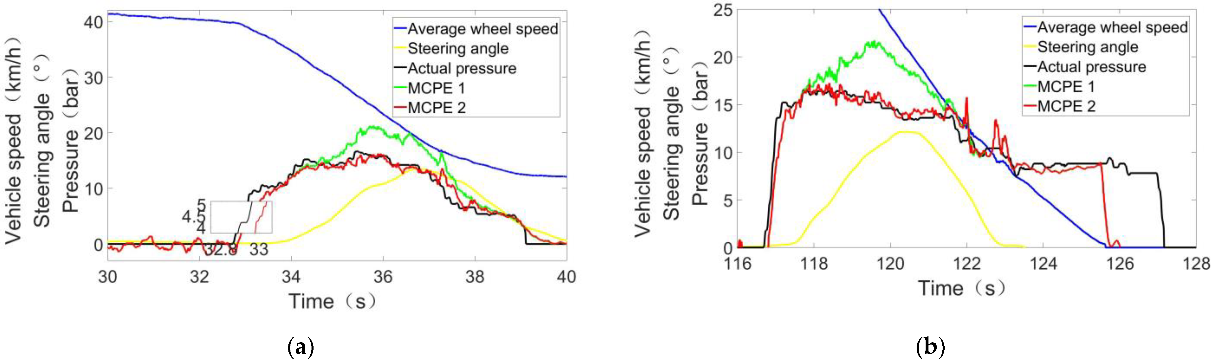
Vehicle tests under steering conditions were conducted. In order to highlight the superiority of the MCPE based on a 5-DOF vehicle model (MCPE 2), it was compared to the MCPE based on longitudinal vehicle dynamics (MCPE 1). The test results are shown in Figure 3, where the vehicle speed is calculated by the average wheel speed, the steering angle is obtained from the EPS, the actual pressure is obtained from the master cylinder pressure sensor, and where MCPE 1 and MCPE 2 correspond to Equation (15) and Equation (14), respectively.

In Figure 3a, before braking, the vehicle is in a coasting state. At this time, the longitudinal acceleration measured by the IMU is the exact driving resistance. Therefore, according to Equation (15), theoretically, the estimated pressure at this time is zero. However, affected by the noise of the IMU signals, the estimated pressure jitters around zero, with a peak-to-peak value of about 3bar. After the start of braking, since the signal of the IMU lags behind the brake pressure, the estimated pressure lags behind the actual pressure, and the lag time is about 100ms. When the vehicle starts steering, as the steering angle increases, MCPE 1 deviates from the actual pressure, while MCPE 2 tracks the actual pressure well, thus proving that the MCPE based on the 5-DOF vehicle model can effectively estimate the brake pressure under both straight and steering conditions.

In Figure 3b, at about 122 s, the noise of the IMU increases due to the uneven road surface, and there is a large jitter in the estimated pressure, with a peak-to-peak value of about 5bar. When the vehicle speed is reduced to zero at about 126 s, the output signal of the IMU keeps zero, and both MCPE 1 and MCPE 2 are invalid.

From the above analysis, it can be seen that although the MCPE based on vehicle dynamics can be extended to steering conditions by adopting the 5-DOF vehicle model, it is still limited by signal noise, road conditions, and algorithm principles. There are still jitter, delay, and condition limitations in the estimated pressure.

4. Pressure-Position Model

The scheme of the EHB is shown in Figure 4 [24]. Under normal braking, the permanent magnet synchronous motor (PMSM) is adopted as the power source, which pushes the master cylinder piston to build pressure through the worm–worm gear and pinion–rack reductions. The electronic control unit (ECU) analyzes the target pressure according to the pedal strokes and performs closed-loop control of the master cylinder pressure based on the master cylinder pressure sensor [33].

Thanks to the angular position sensor of the rotor built in the PMSM, we can estimate the pressure of the master cylinder based on the derived rack position and the pressure–position relationship of the hydraulic circuit.

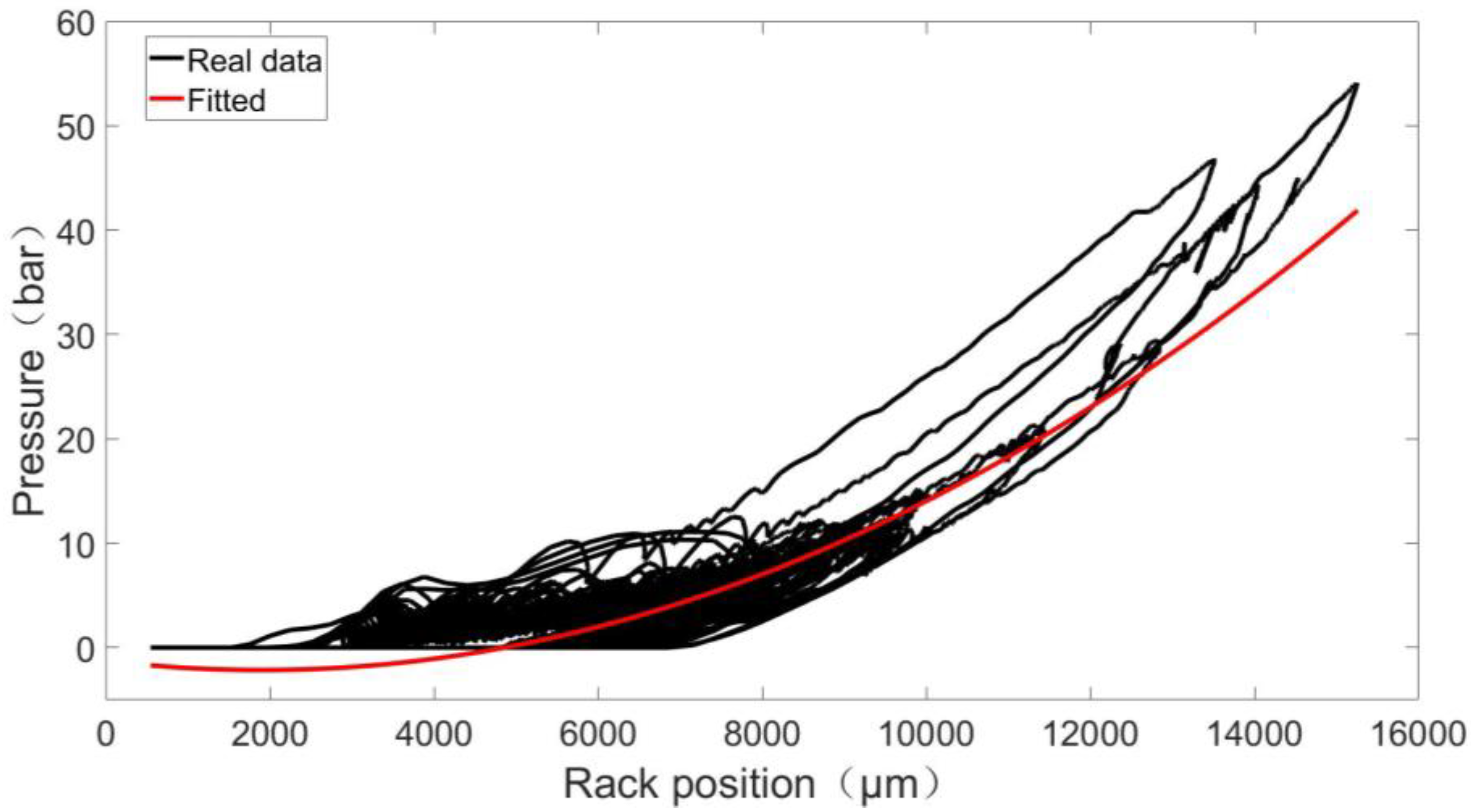
During the braking process, the pipelines expend [34], the caliper deforms [35], and the free gas in the brake fluid is compressed and dissolved [36], which contributes to the pressure–position relationship. The pressure–position relationship is affected by many factors, which are difficult to accurately modeled. Existing studies have shown that the pressure–position relationship has strong nonlinearity (i.e., hysteresis) and time-varying characteristics (brake pad wear, rack speed, etc.). In this article, the pressure–position relationship of a light commercial vehicle (not the test vehicle in Figure 1) under different brake pad wear levels is tested, as shown in Figure 5.

As it can be seen, there is a dead zone of about 6mm in the pressure–position relationship due to gaps in the hydraulic circuit. As the brake pad wears, the pressure–position relationship “softens”, and it takes greater rack displacement to build the same pressure. Moreover, the pressure–position relationship shows hysteresis characteristics. Under the same rack position, the pressure in the pressurization process is greater than that in the depressurization process.

In Ref [37], tests under different rates of motor torque were conducted, and a novel dynamic pressure–position model was proposed as Equation (16).

$$p=a+bx+c{x}^2+d\dot{x}$$

(16)

where $a$, $b$, $c$, and $d$ denote the coefficient; $x$ denotes the rack position; $\dot{x}$ denotes the rack speed; $a+bx+c{x}^2$ represents the “average value” or the “static part” of the pressure–position curve; and $d\dot{x}$ represents the “hysteresis” or the “dynamic part” caused by different rack speed.

Experimental results show that compared to the traditional pressure–position model shown in Equation (17), which is adopted by almost all previous studies in the literature, the dynamic model can render hysteresis and speed influence effect more accurately. In addition, when the rack position and rack speed are used as input, the output pressure of the dynamic model has a faster response speed than the static model [37].

$$p=a+bx+c{x}^2$$

(17)

Although the state-of-the-art pressure–position model can characterize hysteresis and the speed influence effect, when the brake pad is worn down, the “average value” of the pressure–position relationship changes, and the dynamic pressure–position model with a fixed coefficient will not be robust.

5. MCPE Based on Signal Fusion

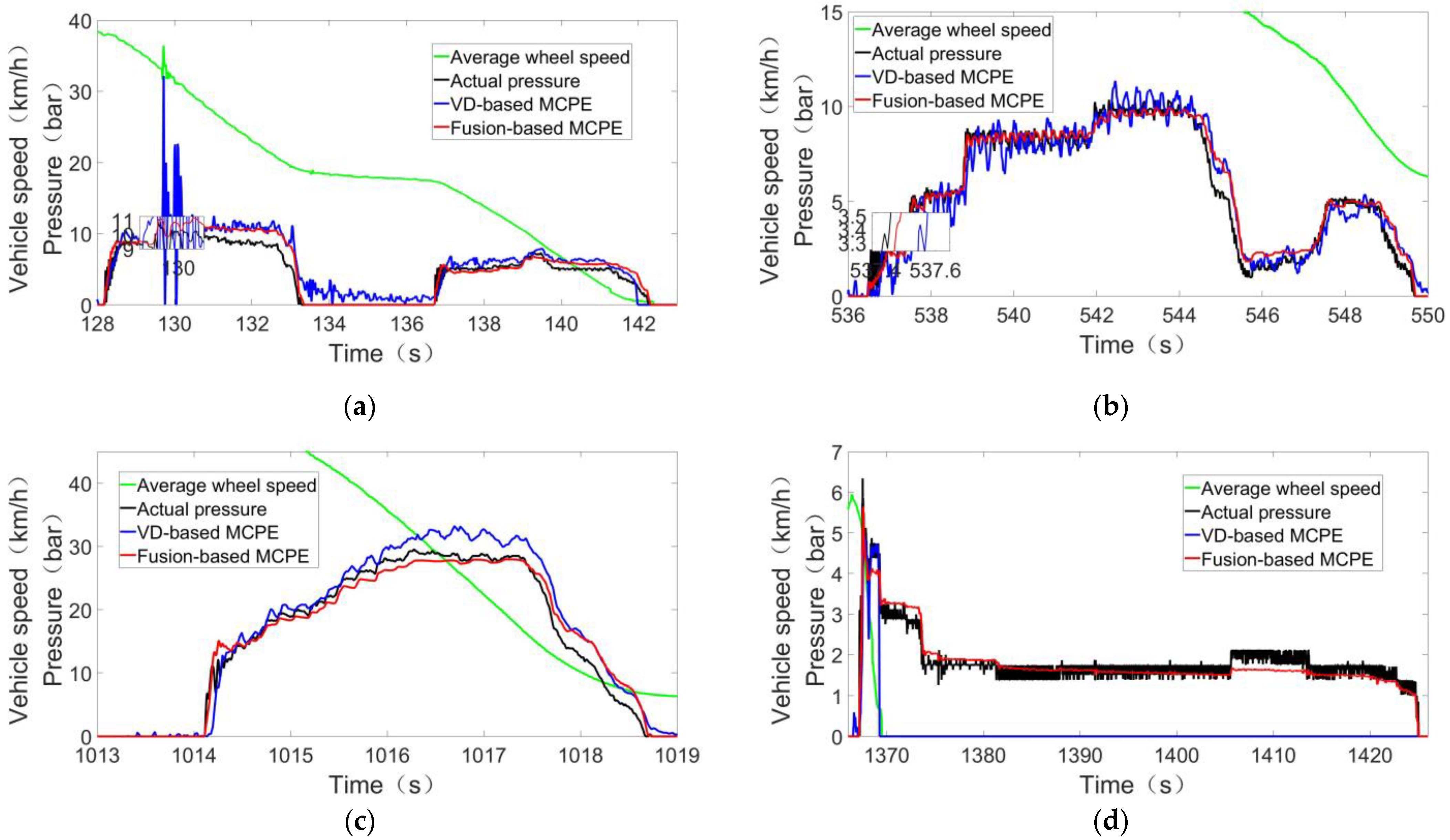
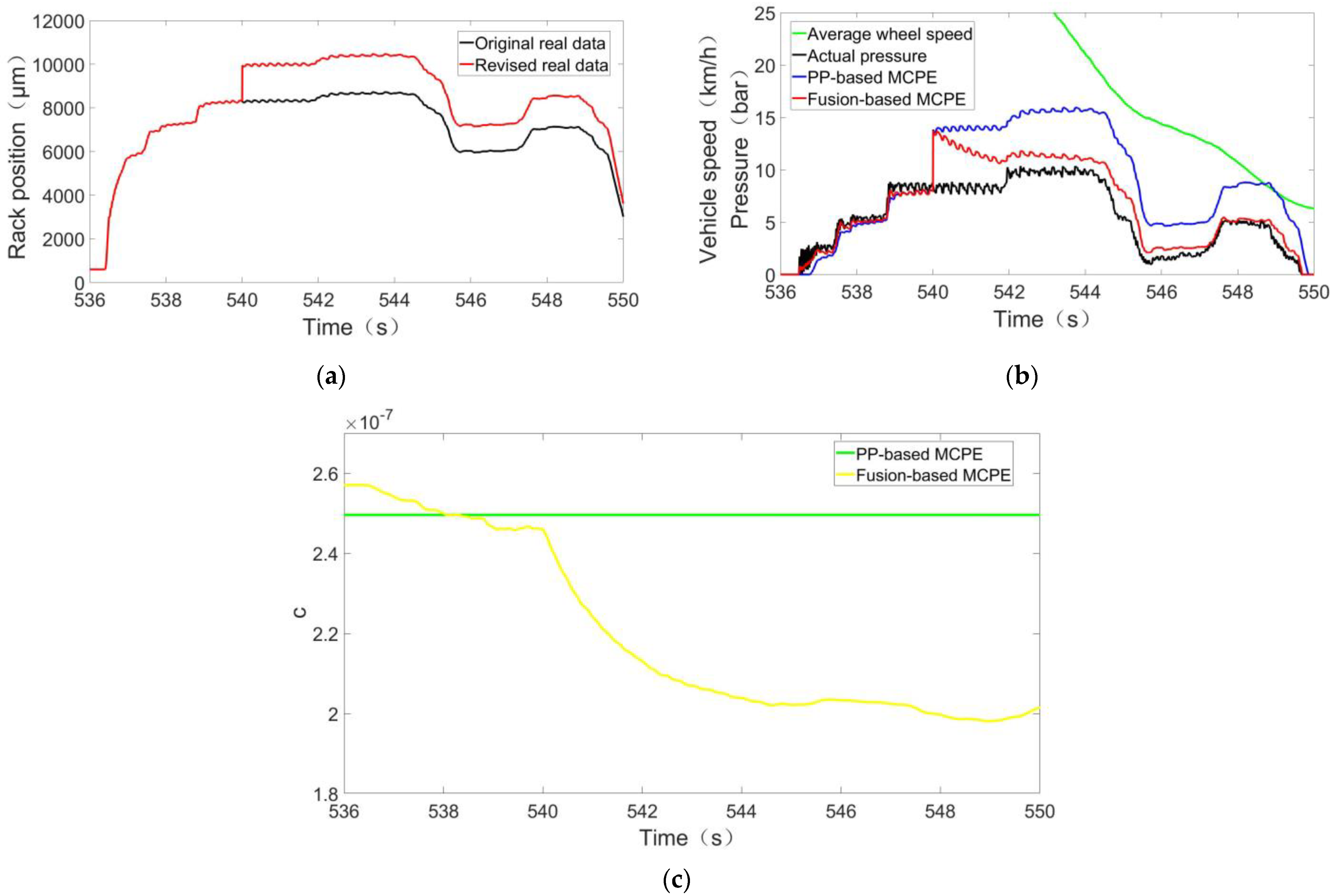
The vehicle dynamics-based MCPE (VD-based MCPE) has many limitations (sensor noise, delay, road conditions, vehicle speed being zero, etc.), but the “average value” of the estimated pressure tracks the actual value very well. Although the pressure–position model based MCPE (PP-based MCPE) is simple and straightforward, it is not robust enough to prevent brake pad wear. Therefore, this article proposes a MCPE based on signal fusion (fusion-based MCPE), in which the coefficients of the pressure–position model are updated by the pressure estimated by the VD-based MCPE based on RLS, and the updated pressure–position model is finally adopted to estimate the brake pressure.

5.1. Principle of the RLS

Suppose $x=\left[\begin{array}{cccc}1& x& x^2& \dot{x}\end{array}\right]$, $\varphi =\left[\begin{array}{c}a\\ b\\ c\\ d\end{array}\right]$, the pressure–position model can be expressed by Equation (18):

$$p=x\varphi$$

(18)

Suppose ${\widehat{p}}_{VD}$ denotes the estimated pressure based on VD-based MCPE, as shown in Equation (19):

$${\widehat{p}}_{VD}=\frac{\left(-M{a}_{x\_IMU}-F_r-F_w\right)L\mathit{cos}\delta -M{a}_{y\_IMU}{L}_r\mathit{sin}\delta -I{\dot{\omega }}_{IMU}\mathit{sin}\delta }{\left(k_{fl}+k_{fr}\right)L+\left(k_{rl}+k_{rr}\right)L\mathit{cos}\delta }r$$

(19)

Since the “average value” of ${\widehat{p}}_{VD}$ is accurate, we hope that the fitted pressure–position model $x\widehat{\varphi }$ is as close to ${\widehat{p}}_{VD}$ as possible. This article adopts the LS method [38] to solve this problem. In a linear system, this is equivalent to finding $\widehat{\varphi }\left(k\right)$ which causes the target function $V\left(\widehat{\varphi }\left(k\right),k\right)$ to obtain the smallest value, as shown in Equation (20):

$$V\left(\widehat{\varphi }\left(k\right),k\right)=\frac{1}{2}{{\displaystyle \sum _{i=1}^k\left({\widehat{p}}_{VD}\left(i\right)-x\left(i\right)\widehat{\varphi }\left(k\right)\right)}}^2$$

(20)

where $k$ denotes the current sampling time. When Equation (20) obtains its smallest value, $\widehat{\varphi }\left(k\right)$ can be solved as Equation (21):

$$\widehat{\varphi }\left(k\right)={\left(X{\left(k\right)}^{T}X\left(k\right)\right)}^{-1}X{\left(k\right)}^{T}Y\left(k\right),$$

(21)

where $X{\left(k\right)}^T=\left[\begin{array}{l}x\left(1\right)\hfill \\ \hfill ⋮\hfill \\ x\left(k\right)\hfill \end{array}\right]$, $Y\left(k\right)=\left[\begin{array}{l}{\widehat{p}}_{VD}\left(1\right)\hfill \\ \hfill ⋮\hfill \\ {\widehat{p}}_{VD}\left(k\right)\hfill \end{array}\right]$. There are two things that need to be pointed out. First, $\widehat{\varphi }\left(k\right)$ is the optimal solution to all of the historic data for $x$ and ${\widehat{p}}_{VD}$; therefore, when the actual pressure–position relationship changes, a certain amount of new data (equivalent to a certain amount of time) is needed for $\widehat{\varphi }\left(k\right)$ to converge to the real value. That is, the convergence speed of the LS is slow. Second, with the increase of $k$, the calculation burden of $\widehat{\varphi }\left(k\right)$ will be heavier, so the storage capacity and computing capacity of the controller are very demanding, and it is not feasible to be applied in engineering.

The first problem can be solved by adopting a LS with a forgetting factor. By adding the forgetting factor to the LS, the data that are farther away from the current moment will occupy a smaller proportion; thus, the convergence speed of the LS is improved. The target function is represented as Equation (22).

$$V\left(\widehat{\varphi }\left(k\right),k\right)=\frac{1}{2}{{\displaystyle \sum _{i=1}^k{\lambda }^{k-i}\left({\widehat{p}}_{m\_pre}\left(i\right)-x\left(i\right)\widehat{\varphi }\left(k\right)\right)}}^2,$$

(22)

For the second problem, the calculation of $\widehat{\varphi }\left(k\right)$ can be transformed into a recursive form. The recursive least square with a forgetting factor can be expressed as Equation (23):

$$\begin{array}{c}\widehat{\varphi }\left(k\right)=\widehat{\varphi }\left(k-1\right)+K\left(k\right)\left[{\widehat{p}}_{VD}\left(k\right)-x\left(k\right)\widehat{\varphi }\left(k-1\right)\right]\\ K\left(k\right)=\frac{P\left(k-1\right)x^T\left(k\right)}{\lambda +x\left(k\right)P\left(k-1\right)x^T\left(k\right)}\\ P\left(k\right)=\frac{1}{\lambda }\left[I-K\left(k\right)x\left(k\right)\right]P\left(k-1\right)\end{array},$$

(23)

where $K\in {ℝ}^{4\times 1}$ denotes the gain; $P\in {ℝ}^{4\times 4}$ denotes the covariance matrix; and $\lambda \in \left(0,1\right)$ denotes the forgetting factor. Finally, the updated pressure–position model is adopted to estimate the brake pressure, as seen in Equation (24):

$${\widehat{p}}_{final}\left(k\right)=x\left(k\right)\widehat{\varphi }\left(k\right)$$

(24)

5.2. Initial Value of the RLS

It can be seen from Equation (23) that the operation of the RLS requires a given initial value of $\widehat{\varphi }\left(k\right)$ and $P\left(k\right)$, that is, $\widehat{\varphi }\left(0\right)$ and $P\left(0\right)$. An appropriate $\widehat{\varphi }\left(0\right)$ and $P\left(0\right)$ can speed up the convergence speed of the algorithm. To this end, this article uses the collected data from the real vehicle test in [24] to fit the pressure–position model by means of LS to obtain $\widehat{\varphi }\left(0\right)$ and $P\left(0\right)$. The collected data, including vehicle speed, brake pressure, rack position, and rack speed with a sampling time of 10ms, are shown in Figure 6.

The data for the brake pressure, rack position, and rack speed should be selected when the brake pressure is greater than zero, and Equations (25) and (26) should be used to calculate $\widehat{\varphi }\left(0\right)$ and $P\left(0\right)$.

$$\widehat{\varphi }\left(0\right)={\left(X{\left(n\right)}^{T}X\left(n\right)\right)}^{-1}X{\left(n\right)}^{T}Y\left(n\right),$$

(25)

$$P\left(0\right)={\left(X{\left(n\right)}^{T}X\left(n\right)\right)}^{-1},$$

(26)

where $X{\left(n\right)}^T=\left[\begin{array}{l}x\left(1\right)\hfill \\ \hfill ⋮\hfill \\ x\left(n\right)\hfill \end{array}\right]$, $Y\left(n\right)=\left[\begin{array}{l}p\left(1\right)\hfill \\ \hfill ⋮\hfill \\ p\left(n\right)\hfill \end{array}\right]$, $n$ denotes the number of the selected data. The results are shown in Equation (27) and Equation (28), respectively.

$$\widehat{\varphi }\left(0\right)=\left[\begin{array}{c}-1.261\\ -9.396\times {10}^{-4}\\ 2.469\times {10}^{-7}\\ 0.5436\end{array}\right],$$

(27)

$$P\left(0\right)=\left[\begin{array}{cccc}5.418\times {10}^{-21}& 5.418\times {10}^{-21}& 5.418\times {10}^{-21}& 5.418\times {10}^{-21}\\ 5.418\times {10}^{-21}& 5.418\times {10}^{-21}& 5.418\times {10}^{-21}& 5.418\times {10}^{-21}\\ 5.357\times {10}^{-21}& 5.357\times {10}^{-21}& 5.357\times {10}^{-21}& 5.357\times {10}^{-21}\\ 5.022\times {10}^{-21}& 5.022\times {10}^{-21}& 5.022\times {10}^{-21}& 5.022\times {10}^{-21}\end{array}\right],$$

(28)

The fitted pressure–position model (i.e., $p\left(k\right)=x\left(k\right)\varphi \left(0\right)$) and the real data are shown in Figure 7. As it can be seen, the fitted model can essentially represent the average value of the real date. Note that the fitted model in Figure 7 is $p=-1.261-9.396\times {10}^{-4}x+2.469\times {10}^{-7}{x}^2$, for there is no dimension to add $0.5436\dot{x}$ in Figure 7.

5.3. Condition Setting for Updating

When $\widehat{\varphi }\left(0\right)$, $P\left(0\right)$, and real-time ${\widehat{p}}_{VD}\left(k\right)$ and $x\left(k\right)$ are given, Equation (23) can continue to run and update $\widehat{\varphi }\left(k\right)$ and $P\left(k\right)$. However, the purpose of this article is to fit the coefficients of the pressure model; that is, the data point $\left({\widehat{p}}_{VD}\left(k\right),x\left(k\right)\right)$ can only be used when they are near the actual pressure–position curve. Therefore, just as when calculating $\widehat{\varphi }\left(0\right)$ and $P\left(0\right)$ in 5.2, only data with a pressure greater than zero are selected. It is necessary to filter the data point $\left({\widehat{p}}_{VD}\left(k\right),x\left(k\right)\right)$ before updating $\widehat{\varphi }\left(k\right)$. Unfortunately, for EHB without a pressure sensor, the selection criteria of pressure greater than zero are no longer applicable. For this reason, this article proposes a new screening method. For the sake of analysis, suppose the vehicle is on a straight and flat road.

When the vehicle stops, $M{a}_{x\_IMU}=0$,${\widehat{p}}_{VD}\left(k\right)=\frac{-F_r-F_w}{k_{fl}+k_{fr}+k_{rl}+k_{rr}}r<0$. Obviously, the data point $\left({\widehat{p}}_{VD}\left(k\right),x\left(k\right)\right)$ cannot be used to update $\widehat{\varphi }\left(k\right)$ and $P\left(k\right)$.

When coasting, $M{a}_{x\_IMU}=-F_r-F_w$, ${\widehat{p}}_{VD}\left(k\right)=\frac{-M{a}_{x\_IMU}-F_r-F_w}{k_{fl}+k_{fr}+k_{rl}+k_{rr}}r=0$. According to the control logic of EHB, when the brake pedal is not depressed, the rack will be pushed to the zero position. Therefore, the data point $\left({\widehat{p}}_{VD}\left(k\right),x\left(k\right)\right)$ is not on the effective section of the pressure–position curve at that moment; therefore, the pressure–position model cannot be updated while coasting.

When accelerating, $M{a}_{x\_IMU}>-F_r-F_w$, ${\widehat{p}}_{VD}\left(k\right)=\frac{-M{a}_{x\_IMU}-F_r-F_w}{k_{fl}+k_{fr}+k_{rl}+k_{rr}}r<0$. This is the same as when the vehicle stops.

When the brake pedal is stepped on and when the rack crosses the dead zone and builds pressure, $M{a}_{x\_IMU}<-F_r-F_w$, ${\widehat{p}}_{VD}\left(k\right)=\frac{-M{a}_{x\_IMU}-F_r-F_w}{k_{fl}+k_{fr}+k_{rl}+k_{rr}}r>0$. In addition, when the rack has crossed the dead zone and is in the effective zone, the data point $\left({\widehat{p}}_{VD}\left(k\right),x\left(k\right)\right)$ is suitable to update $\widehat{\varphi }\left(k\right)$ and $P\left(k\right)$ at this time.

In summary, the pressure–position model is only updated when the vehicle speed is greater than a certain threshold and when the rack position is greater than a certain threshold, as in Equation (29).

$$\begin{array}{l}\widehat{\varphi }\left(k\right)=\{\begin{array}{l}\widehat{\varphi }\left(k-1\right),\hspace{1em}\hspace{1em}\hspace{1em}\hspace{1em}\hspace{1em}\hspace{1em}u<u_{threshold} or x<x_{threshold}\\ \widehat{\varphi }\left(k-1\right)+K\left(k\right)\left[{\widehat{p}}_{VD}\left(k\right)-x\left(k\right)\widehat{\varphi }\left(k-1\right)\right], otherwith\end{array}\\ K\left(k\right)=\frac{P\left(k-1\right)x^T\left(k\right)}{\lambda +x\left(k\right)P\left(k-1\right)x^T\left(k\right)}\\ P\left(k\right)=\{\begin{array}{l}P\left(k-1\right),\hspace{1em}u<u_{threshold} or x<x_{threshold}\\ \frac{1}{\lambda }\left[I-K\left(k\right)x\left(k\right)\right]P\left(k-1\right), otherwith\end{array}\end{array},$$

(29)

where $u_{threshold}$ and $x_{threshold}$ denote the vehicle speed threshold and the rack position threshold, respectively. Note that by updating the pressure–position model with the filtered data pairs, a more accurate pressure–position model is expected to be obtained so that when the rack is in the dead zone, the estimated pressure must be negative, as shown in Figure 7. To this end, the estimated pressure is limited by Equation (30).

$${\widehat{p}}_{final}\left(k\right)=\{\begin{array}{l}x\left(k\right)\widehat{\varphi }\left(k\right),x\left(k\right)\widehat{\varphi }\left(k\right)>0\\ 0,\hspace{1em}\hspace{1em}\hspace{1em}\hspace{1em}\hspace{1em}otherwith\end{array}$$

(30)

Finally, the fusion-based MCPE can be represented by Equations (19) and (27)–(30).

6. Validation of the Proposed Fusion-Based MCPE

Based on the experimental data in [24], the proposed fusion-based MCPE is verified by the MATLAB/Simulink platform, and the simulation step is 5 ms. The verification consists of two parts. The first part verifies that the fusion-based MCPE outperforms the VD-based MCPE in terms of smoothness, delay time, robustness to road conditions, and adaptability to parking conditions. The second part verifies that the fusion-based MCPE outperforms the PP-based MCPE in terms of robustness to brake pad wear. The parameter settings of the fusion-based MCPE are as they are seen in

Table 2. Parameter settings of the fusion-based MCPE.

Item	Value
Vehicle speed threshold $u_{threshold}$	3.6 km/h
Rack position threshold $x_{threshold}$	6000 μm
Forgetting factor $\lambda$	0.999

.

6.1. Normal Driving Conditions

Simulations based on experimental data under normal driving conditions were conducted, the results are shown in Figure 8.

In Figure 8a, when the vehicle encounters a speed bump at about 130s, there is severe jitter in the VD-based MCPE with a peak-to-peak value of 60bar. In contrast, the fusion-based MCPE can still work smoothly, with a peak-to-peak value of only 1.2bar. In addition, when the vehicle is coasting, the estimated pressure of the fusion-based MCPE is zero, while the estimated pressure of VD-based MCPE jitters around zero. In Figure 8b, under normal driving conditions, the fusion-based MCPE is much more stable than the VD-based MCPE, and the RMSE of them are 0.3597bar and 0.9182bar, respectively. In addition, in terms of delay time, the fusion based MCPE is much smaller than the VD-based MCPE due to the fast response of the novel dynamic pressure–position model proposed in [37]; the former is only 25ms, and the latter exceeds 100ms. The brake pressure under normal driving conditions is generally not more than 30bar. Figure 8c shows that under 30bar, the proposed fusion-based MCPE can still estimate the brake pressure precisely. Figure 8d represents the condition where the vehicle stops at a traffic intersection. After the vehicle speed is reduced to zero, the driver still brakes with a small amount of brake pressure. It can be seen in Figure 8d that after the vehicle stops, the VD-based MCPE fails, while the fusion-based MCPE can estimate the brake pressure consistently and accurately. The evolution of the coefficient $c$ of the pressure–position model is shown in Figure 8e. Note that $c$ is the coefficient of the square term of the rack position and that its value has a great influence on the pressure–position model. In Figure 8e, when the vehicle speed is about to decrease to zero, the RLS stops updating $\widehat{\varphi }\left(k\right)$, and $c$ remains unchanged, thus ensuring that after the vehicle speed is reduced to zero, the fusion-based MCPE can continue to estimate the brake pressure.

6.2. Brake Pad Wear

In order to verify the robustness of the fusion-based MCPE to brake pad wear, the fusion-based MCPE was compared with the PP-based MCPE with the fixed coefficient as Equation (31).

$$p\left(k\right)=x\left(k\right)\varphi \left(0\right)$$

(31)

When the brake pad is worn, the pressure–position curve becomes “soft”; that is, the same pressure corresponds to a larger rack position. Therefore, in order to simulate the brake pad wear, the experimental data of the rack position are set as 1.2 times of the original at 540s in the simulation, the result of which is shown in Figure 9.

Figure 9a shows that the original rack position is changed to 1.2 times of the original value at 540 s. In Figure 9b, after 540 s, as expected, the estimated pressure of the PP-based MCPE is always greater than the actual value, while the fusion-based MCPE can gradually converge to the actual value. Figure 9c shows that after 540 s, since the RLS continuously updates $\widehat{\varphi }\left(k\right)$ according to the new data point of $\left({\widehat{p}}_{VD}\left(k\right),x\left(k\right)\right)$, $c$ gradually decreases and converges to a stable value at about 548 s. This proves the robustness of the fusion-based MCPE to brake pad wear.

7. Conclusions

For the problem that a MCPE based on longitudinal vehicle dynamics cannot be used in steering conditions, a MCPE based on a 5-DOF vehicle model was proposed. Real vehicle test showed that the proposed method can effectively estimate the brake pressure in both straight and steering conditions.

Aiming to solve the problem of noise and delay in the VD-based MCPE and the poor robustness of the PP-based MCPE, a fusion-based MCPE was proposed. A RLS with a forgetting factor was adopted to update the coefficients of the pressure–position model, and the brake pressure was then estimated by the updated pressure–position model. Simulations were conducted based on the vehicle test data. The results show that the fusion-based MCPE can estimate the brake pressure accurately, smoothly, and quickly under various working conditions. Specifically, compared to a VD-based MCPE, the RMSE is reduced from 0.9182 bar to 0.3597 bar, and the delay time is reduced from 100ms to 25 ms. In addition, due to the reasonable setting of the enabling conditions of the RLS, the updated pressure–position model is more accurate. Therefore, when the brake is not applied, the rack position is zero. At this time, the estimated pressure is negative which avoids the problem of the VD-based MCPE oscillating near zero. Moreover, when the vehicle speed drops to zero, the RLS stops updating, so the brake pressure can be estimated smoothly and continuously when the vehicle is in stationary mode. Finally, since the fusion algorithm will constantly update the pressure–position model based on new data, when the pressure–position model is changed due to brake pad wear, the RLS will automatically update the pressure–position model to the worn state; therefore, the robustness of the fusion-based MCPE is ensured.