Computational Intelligence-Based Prognosis for Hybrid Mechatronic System Using Improved Wiener Process

Abstract

In this article, a fast krill herd algorithm is developed for prognosis of hybrid mechatronic system using the improved Wiener degradation process. First, the diagnostic hybrid bond graph is used to model the hybrid mechatronic system and derive global analytical redundancy relations. Based on the global analytical redundancy relations, the fault signature matrix and mode change signature matrix for fault and mode change isolation can be obtained. Second, in order to determine the true faults from the suspected fault candidates after fault isolation, a fault estimation method based on adaptive square root cubature Kalman filter is proposed when the noise distributions are unknown. Then, the improved Wiener process incorporating nonlinear term is developed to build the degradation model of incipient fault based on the fault estimation results. For prognosis, the fast krill herd algorithm is proposed to estimate unknown degradation model coefficients. After that, the probability density function of remaining useful life is derived using the identified degradation model. Finally, the proposed methods are validated by simulations.

1. Introduction

Hybrid mechatronic systems, which include interacting continuous and discrete dynamics, are widely used in modern industrial systems, such as automobile, chemical plant, and aerospace engineering [1,2]. As their complexities increase, higher demand on safety and reliability requires more accurate fault diagnosis and failure prognosis which could provide effective means for system maintenance. Consequently, it is important to detect and isolate system faults as soon as possible and then considerable economic losses can be avoided [3,4,5]. Since recent years, many valuable works have been reported in the hybrid system fault diagnosis and prognosis fields [6,7,8,9,10]. Among these works, discrete event system model-based methods (e.g., Petri net and automaton) are widely investigated. The timed Petri net model is used for mode tracking and fault diagnosis of hybrid systems [6]. This model can only depict the temporal discrete event degradation of the hybrid system because the continuous dynamics is neglected. The main problem of this method is that domain-specific knowledge is required to build the fault–symptom table. In addition, training data obtained from reliability testing are needed to compute the individual faults prior probability distributions. The hybrid automaton model is utilized for fault diagnosis of hybrid systems based on structured residuals [7]. The hybrid automaton model consists of finite state automaton and continuous state-space model. The continuous state-space model is used to derive structured residuals for fault detection. The structured residuals can generate the fault signatures for fault isolation. However, for complex hybrid systems with many modes, this method needs to derive a large number of state-space models. Therefore, it is difficult to design fault diagnosis algorithms and real-time implementation under this situation. Fortunately, hybrid bond graph (HBG), which is a graphical tool only, utilizes a set of unified equations (i.e., global analytical redundancy relations (GARR)) for fault diagnosis where information of all modes and physical component faults are incorporated [10]. According to GARRs, the fault signature matrix (FSM) and mode change signature matrix (MCSM) can be established, based on which the isolation of unexpected mode change and component fault can be carried out.

In some cases, the estimations of fault parameters are needed to evaluate the fault severity (e.g., fault severity is required for fault tolerant control) and at the same time refine the set of fault candidates (SFC) if some faults in SFC are non-isolable. The Kalman filter (KF) is a popular method for fault parameter estimation of linear systems with Gaussian noise where the fault parameter is treated as a special state. It generates recursive estimations of state vectors by optimally weighting information from the system dynamic model and current measurements [11]. However, KF is geared toward linear systems [12]. To deal with nonlinear systems, extended Kalman filter (EKF) is developed, and this method linearizes the nonlinear systems using the Jacobian matrix, which may reduce the estimation accuracy [13]. To ameliorate the filter performance, some more efficient methods, e.g., unscented Kalman filter (UKF) and cubature Kalman filter (CKF), are proposed. The advantage of these methods over EKF lies in that the calculation of Jacobian matrix is not required (e.g., UKF directly propagates the nonlinear function through unscented transformation and CKF uses cubature points to approximate the variance and mean). As a result, UKF and CKF can achieve more accurate filtering performance for strongly nonlinear systems [14,15]. However, UKF may lead to uncertain solution because it requires the weight of the central sampling point to be positive [16]. Likewise, the covariance matrix of CKF cannot be decomposed if its positive definiteness is not ensured, which may obstruct the algorithm implementation. To solve the above problem, the square root cubature Kalman filter (SRCKF) which utilizes the square root of the covariance matrix is proposed to guarantee the non-negative definiteness of the covariance matrix [15]. Nevertheless, it is not a trivial task to properly set the filter noise covariances for SRCKF.

The health monitoring not only needs to diagnose the fault, but also needs to prevent the failure by predicting the remaining useful life (RUL). Roughly speaking, RUL prediction (or prognosis) methods are mainly composed of model-based approaches and data-driven approaches [17,18,19,20,21]. A model-based sequential prognosis method is developed for an electric scooter in the presence if intermittent fault [17]. However, it is challenging to obtain the accurate mathematical model of the degradation process which makes the application of model-based prognosis methods difficult. Therefore, many literatures investigate data-driven approaches which rely on the quality and quantity of history data as alternatives. Yang et al. propose an intelligent RUL prediction method based on a double convolutional neural network model architecture [19]. Both the above model-based and data-driven methods use deterministic degradation models where the randomness of the degradation process is not considered [10,17,18,19]. To overcome this shortcoming, the Wiener process, which incorporates stochastic nature in degradation models, is proved to be a suitable tool [20]. In [21], Wiener process with linear drift is utilized for the preventive maintenance of microelectromechanical systems. However, most degradation processes are nonlinear where the standard Wiener process may not be a promising solution.

To cope with the aforementioned difficulties, this article proposes a new prognosis method based on improved Wiener process for the hybrid mechatronic system. The main contributions of this article are threefold:

(1) An adaptive square root cubature Kalman filter (ASRCKF) which can adaptively estimate the unknown noise distributions is proposed to accurately estimate the fault parameter.

(2) An improved Wiener process with nonlinear term is developed to capture the degradation of incipient fault.

(3) A prognosis method using fast krill herd (FKH) algorithm is proposed where the FKH is developed to estimate the degradation model coefficients based on the identified fault data from fault estimation module.

The remainder of this article is organized as follows. Section 2 models the hybrid mechatronic system based on the diagnostic hybrid bond graph (DHBG) theory. In Section 3, the ASRCKF-based fault estimation is introduced. Section 4 presents the RUL prediction based on improved Wiener process whose coefficients are estimated by FKH. Section 5 analyzes the simulation results. Finally, the concluding remarks are given in Section 6.

2. FDI Based on DHBG Model

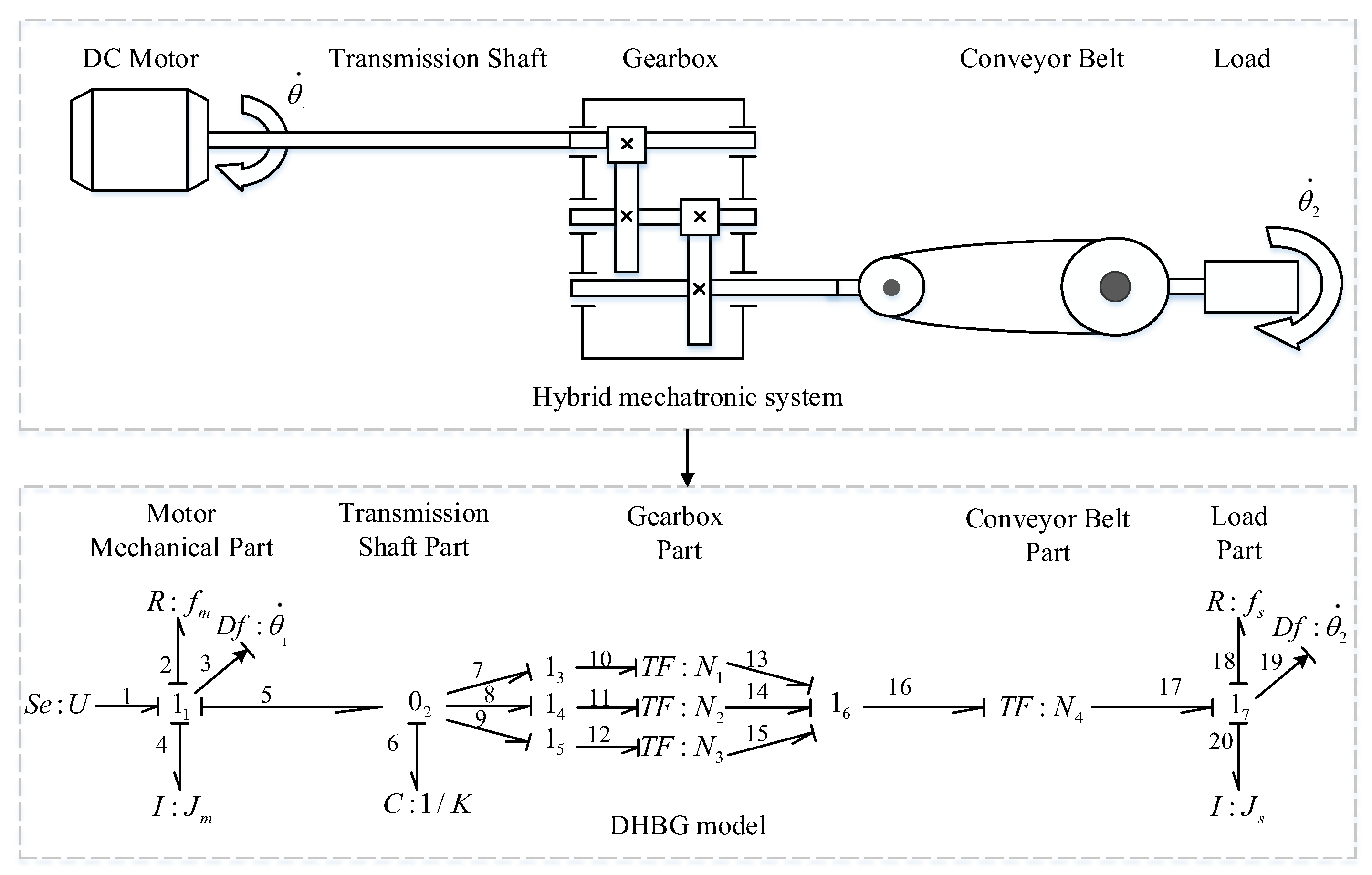
Due to the capability in modeling systems with multi-energetic domains, bond graph (BG) theory, which is based on energy conservation law, is a reasonable choice for fault diagnosis and isolation (FDI) of complex mechatronic systems [4]. In BG methodology, different types of multiport elements are utilized to model the physical components and their behaviors in a variety of energy domains. Generic BG elements consist of source elements ($Sf$ and $Se$), dissipative element (R), storage elements (C and I), two junctions (0 junction and 1 junction), and two transducers ($TF$ and $GY$) [17]. The half arrow bond is used to connect these generic BG elements. For each bond, there are two power variables (effort e and flow f) which can describe the energy exchange between different elements. In addition, there is a perpendicular stroke at one end of a bond to represent the cause and effect relation between power variables. In summary, the BG modeling uses the generic BG elements and bonds with causalities to describe the behaviors of physical system. In Figure 1, the hybrid mechatronic system which includes continuous and discrete states consists of several subsystems. Thus, it is preferred to use HBG to model the hybrid mechatronic system in a compact manner. The basic BG method is applied to the modeling of continuous systems, while the HBG extends the capability of basic BG to model hybrid systems with the aid of controlled junctions, by which the dynamic characteristic of discrete states characterized by modes can be described. For the purpose of FDI, the sequential causality assignment procedure for hybrid system diagnosis is developed to achieve DHBG, where the sensor causalities are inverted and controlled junctions are put in preferred causalities [10]. After that, the GARR can be obtained from DHBG.

The DHBG model of the hybrid mechatronic system is shown in Figure 1. The system can be divided into five parts: DC motor, transmission shaft, gearbox, conveyor belt, and load. The model input $Se$:U is an effort source, representing the input torque. The representation of $Se$:U follows the convention of BG modeling where the physical parameter of an element (i.e., U for effort source) is attached to the symbol of the element (i.e., $Se$ for effort source) by a colon. This representation applies to all generic BG elements except junction elements. The DC motor mechanical part is composed of the rotor inertia I:$J_m$ and mechanical friction R:$f_m$. The stiffness K of the transmission shaft is represented by the capacitive element C. The gearbox is modeled by three $TF$ elements with gear ratios $N_1$, $N_2$ and $N_3$. Likewise, the transformer element $TF$ is used to model the conveyor belt with transmission ratio $N_4$. The load is characterized by rotational inertia I:$J_s$ and mechanical friction R:$f_s$. The angular velocities of motor and load are measured by two flow sensors $Df$:${\dot{\theta }}_1$ and $Df$:${\dot{\theta }}_2$.

Analytical redundancy relation (ARR) is a dynamic constraint only containing the known information (i.e., sensor measurements, inputs and physical parameters) of the system. According to the real-time numerical evaluation of ARR (i.e., residual), the fault can be detected if the observed residual exceeds the corresponding threshold. In the DHBG model, the structure and dynamic characteristics of the system are different under diverse modes, and the basic ARR is unable to describe the constraints under different modes in an unified manner. In order to efficiently utilize the residuals generated from DHBG models, the concept of the GARR is introduced. The main distinction between GARR and basic ARR is that GARR carries mode information. The general form of GARR can be represented as follows [22]:

$$G_j\left(a,\theta ,U,D_e,D_f\right)=0,j=1,2\dots n_g$$

(1)

where $G_j$ represents the jth GARR, a is the mode, $\theta$ denotes the physical parameter, U is the system input, and $D_e$ and $D_f$ represent the sensor measurements. In Figure 1, $1_3$, $1_4$, and $1_5$ are controlled junctions and the corresponding mode is $a=\left[a_1{a}_2{a}_3\right]$, where $a_i\in \left\{0,1\right\}$, $i=1,2,3$, and ${\sum }_{i=1}^3{a}_i=1$ (indicates that at any instant only one gear ratio is in operation). In DHBG, the junctions attached with sensors of inverted causality are used to derive the GARR equations. In the causality inversion method, the causality of sensor is inverted and the output of the sensor-attached junction is zero (e.g., $f_3=0$ for junction $1_1$). Thus, the necessary condition of deriving an ARR (i.e., the junction output variable must be measured by a sensor) can be relaxed. In this way, the ARR can be established using the constitutive relation of the sensor-attached junction [17]. For junction $1_1$ connected to the sensor with inverted causality, the constitutive relation can be obtained as follows:

$$e_1-e_2-e_3-e_4-e_5=0$$

(2)

To derive the GARR from junction $1_1$, the unknown variables in (2) should be eliminated by covering the causal paths. Thus, the unknown variables in (2) can be expressed as

$$\begin{array}{cc}\hfill e_1& =U\hfill \\ \hfill e_2& =f_m{f}_2=f_m{\dot{\theta }}_1\hfill \\ \hfill e_3& =0\hfill \\ \hfill e_4& =J_m\frac{d{f}_4}{dt}=J_m\frac{d{\dot{\theta }}_1}{dt}=J_m{\ddot{\theta }}_1\hfill \\ \hfill e_5& =K\int \left[{\dot{\theta }}_1-N_a{N}_4{\dot{\theta }}_2\right]dt\hfill \end{array}$$

(3)

where $N_a={\sum }_{i=1}^3{a}_i{N}_i$ is the gear ratio which is in operation.

Substituting (3) into (2) leads to $GAR{R}_1$ as follows:

$$GAR{R}_1=U-f_m{\dot{\theta }}_1-J_m{\ddot{\theta }}_1-K\int \left({\dot{\theta }}_1-N_a{N}_4{\dot{\theta }}_2\right)dt$$

(4)

For junction $1_7$ with sensor of inverted causality, the constitutive relation can be formulated as

$$e_{17}-e_{18}-e_{19}-e_{20}=0$$

(5)

In the similar way, the unknown variables in (5) can be solved as

$$\begin{array}{cc}\hfill e_{17}& =N_4{e}_{16}=N_a{N}_{4}K\int \left({\dot{\theta }}_1-N_a{N}_4{\dot{\theta }}_2\right)dt\hfill \\ \hfill e_{18}& =f_s{f}_{18}=f_s{\dot{\theta }}_2\hfill \\ \hfill e_{19}& =0\hfill \\ \hfill e_{20}& =J_s\frac{d{f}_{20}}{dt}=J_s\frac{d{\dot{\theta }}_2}{dt}\hfill \end{array}$$

(6)

Substituting (6) into (5) results in $GAR{R}_2$ as follows:

$$GAR{R}_2=N_a{N}_{4}K\int \left({\dot{\theta }}_1-N_a{N}_4{\dot{\theta }}_2\right)dt-f_s{\dot{\theta }}_2-J_s{\ddot{\theta }}_2$$

(7)

when the fault or the unknown mode change occurs, the corresponding GARR will exceed the threshold. Therefore, a binary coherent vector CV $=[c_1\dots c_{n_g}]$ is defined to represent the consistency of GARRs. The decision rule of $c_j$ is defined as follows:

$$c_j=\left\{\begin{array}{cc}1,\hfill & |g_j|>{\iota }_j\hfill \\ 0,\hfill & \mathrm{other}\hfill \end{array}\right.,j=1,2,\cdots ,n_g$$

(8)

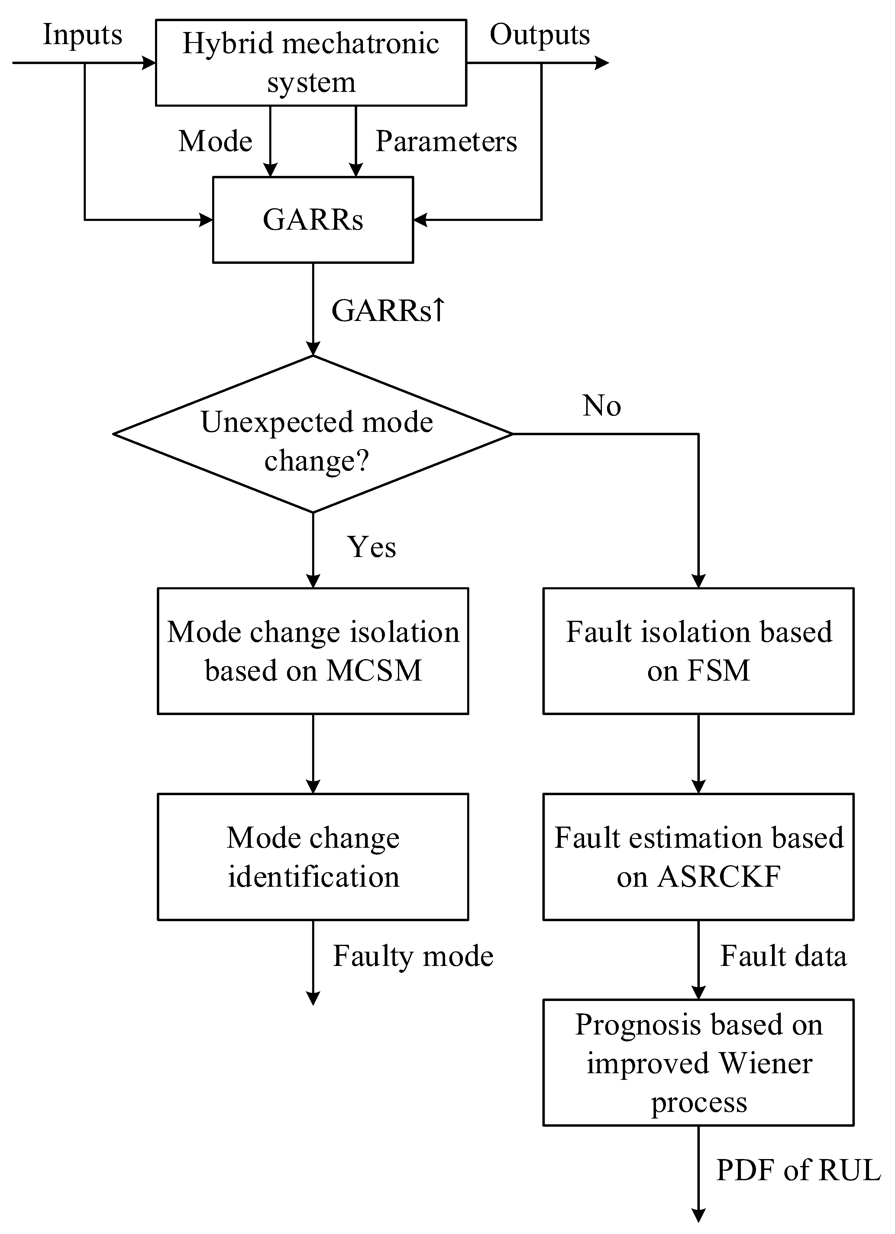
In the developed prognosis method, the first step is to detect and isolate the unexpected mode change by comparing the CV with the MCSM. The MCSM is shown in

Table 1. Mode change signature matrix.

	${\mathit{r}}_1$	${\mathit{r}}_2$	${\mathit{D}}_{\mathit{b}}$
$a_1$	1	1	1
$a_2$	1	1	1
$a_3$	1	1	1

, where $D_b$ represents the detectability. If the unexpected mode change is detected, all possible modes are put in the GARRs. The mode that makes the GARRs consistent is the actual mode. If no unexpected mode change is detected, the nonzero CV is caused by the parameter fault, and the SFC can be obtained by comparing the CV with the FSM in

Table 2. Fault signature matrix.

	${\mathit{r}}_1$	${\mathit{r}}_2$	${\mathit{D}}_{\mathit{b}}$
$f_m$	1	0	1
$J_m$	1	0	1
$f_s$	0	1	1
$J_s$	0	1	1
K	1	1	1
U	1	0	1
$N_4$	1	1	1

. Take an example of the actuator fault in U, CV $=\left[10\right]$, which cannot be caused by the unexpected mode change, is detected upon the fault occurrence. After comparing the CV with FSM, the SFC $=\left\{U,f_m,J_m\right\}$ is obtained. To refine the SFC, the ASRCKF-based fault estimation is enabled, where the possible fault parameters in SFC are treated as special states in the state-space model derived from GARRs. Based on the fault estimation results, the fault data representing the fault parameter degradation can be obtained, by which the coefficients of improved Wiener process-based degradation model can be estimated by the FKH algorithm. Once the degradation model is obtained, the prognosis can be implemented using the predefined failure threshold. The framework of the developed prognosis method is illustrated in Figure 2.

3. Fault Estimation Based on ASRCKF

With the SFC, the next step is to identify the true fault. In this work, the CKF is employed for fault parameter estimation. Compared with the EKF, CKF which uses cubature points to approximate the variance and mean can achieve better filtering performance for some highly nonlinear systems. To avoid the situation that the covariance matrix of CKF cannot be decomposed, the SRCKF is proposed. However, both CKF and SRCKF require the prior statistical characteristics of noises which are usually unavailable in real applications. Motivated by this observation, ASRCKF is proposed to adaptively update the unknown covariance matrix of process noise and measurement noise.

To implement the ASRCKF for the joint estimation of state and fault parameters, the system state $\overline{x}={[{\theta }_1,{\dot{\theta }}_1,{\theta }_2,{\dot{\theta }}_2]}^T$ requires to be augmented as $x_k={[{\theta }_1,{\dot{\theta }}_1,{\theta }_2,{\dot{\theta }}_2,\mathsf{\Phi }]}^T$, where $\mathsf{\Phi }$ represents the vector which contains all fault parameters in the SFC (e.g., U, $f_m$, and $J_m$ if CV $=\left[10\right]$). Consequently, the nonlinear discrete stochastic model can be derived as

$$\left\{\begin{array}{c}{x}_k=f(x_{k-1},w_k)\hfill \\ z_k=h(x_k,v_k)\hfill \end{array}\right.$$

(9)

Before introducing the ASRCKF, it is necessary to describe the cubature point selection strategy. According to the third-degree spherical-radial rule, the cubature points are defined as

$${\xi }_i=\sqrt{\frac{m}{2}}{\left[1\right]}_i,{\omega }_i=\frac{1}{m},i=1,2,\cdots ,m,m=2n$$

(10)

where n is the state dimension of the system and ${\left[1\right]}_i$ is the ith element in the operator space

$$\left[1\right]=\left\{\left[\begin{array}{c}1\hfill \\ 0\hfill \\ ⋮\hfill \\ 0\hfill \end{array}\right],\left[\begin{array}{c}0\hfill \\ 1\hfill \\ ⋮\hfill \\ 0\hfill \end{array}\right],\dots ,\left[\begin{array}{c}0\hfill \\ 0\hfill \\ ⋮\hfill \\ 1\hfill \end{array}\right],\left[\begin{array}{c}-1\\ 0\\ ⋮\\ 0\end{array}\right],\left[\begin{array}{c}0\\ -1\\ ⋮\\ 0\end{array}\right],\dots ,\left[\begin{array}{c}0\\ 0\\ ⋮\\ -1\end{array}\right]\right\},{\left[1\right]}_i\in \left[1\right]$$

(11)

In summary, the ASRCKF can be described as follows.

(1) Initialize state $x_0$ and covariance matrix $P_0$ and factorize the covariance matrix

$$P_{k-1|k-1}=S_{k-1|k-1}{S}_{k-1|k-1}^T,k=1,2,\cdots ,end$$

(12)

(2) Calculate the cubature points of state vector and cubature points of prediction values of state vector

$$X_{i,k-1|k-1}=S_{k-1|k-1}{\xi }_i+{\widehat{x}}_{k-1|k-1},i=1,2,\cdots ,m$$

(13)

$$X_{i,k|k-1}^{*}=f(X_{i,k-1|k-1},w_k),i=1,2,\cdots ,m$$

(14)

(3) Calculate the predicted state vector and the square root factor of the predicted error

$${\widehat{x}}_{k|k-1}=\frac{1}{m}\sum _{i=1}^m{X}_{i,k|k-1}^{*}$$

(15)

$$S_{Q,k|k-1}=Tria\left([X_{k|k-1}^{*},S_{Q,k}]\right)$$

(16)

where $Tria$ denotes a general triangularization algorithm (e.g., the QR decomposition), $S_{Q,k}=chol\left(Q_K\right)$ and $X_{k|k-1}^{*}$ is calculated as

$$X_{k|k-1}^{*}=\frac{1}{\sqrt{m}}[X_{1,k|k-1}^{*}-{\widehat{x}}_{k|k-1},X_{2,k|k-1}^{*}-{\widehat{x}}_{k|k-1},\cdots ,X_{m,k|k-1}^{*}-{\widehat{x}}_{k|k-1}]$$

(4) Calculate the cubature points of predicted state vector and cubature points of prediction values of measurement vector

$$X_{i,k|k-1}=S_{k|k-1}{\xi }_i+{\widehat{x}}_{k|k-1},i=1,2,\cdots ,m$$

(17)

$$Y_{i,k|k-1}=h\left(X_{i,k|k-1}\right)$$

(18)

(5) Calculate the predicted measurement vector and square root factor of the innovation covariance matrix

$${\widehat{z}}_{k|k-1}=\frac{1}{m}\sum _{i=1}^m{Y}_{i,k|k-1}$$

(19)

$$S_{R,k|k-1}=Tria\left([Y_{k|k-1},S_{R,k}]\right)$$

(20)

where $S_{R,k}=chol\left(R_k\right)$ and $Y_{k|k-1}$ is expressed as

$$Y_{k|k-1}=\frac{1}{\sqrt{m}}[Y_{1,k|k-1}-{\widehat{z}}_{k|k-1},Y_{2,k|k-1}-{\widehat{z}}_{k|k-1},\cdots ,Y_{m,k|k-1}-{\widehat{z}}_{k|k-1}]$$

(6) Calculate the cross-covariance matrix and Kalman gain matrix

$$P_{k|k-1}=X_{k|k-1}{Y}_{k|k-1}^T$$

(21)

$$K_k=(P_{k|k-1}/S_{R,k|k-1}^T)/S_{R,k|k-1}$$

(22)

where $X_{k|k-1}$ is expressed as

$$X_{k|k-1}=\frac{1}{\sqrt{m}}[X_{1,k|k-1}-{\widehat{x}}_{k|k-1},X_{2,k|k-1}-{\widehat{x}}_{k|k-1},\cdots ,X_{m,k|k-1}-{\widehat{x}}_{k|k-1}]$$

(7) Update the state estimation and calculate the square root factor of the error covariance matrix

$${\widehat{x}}_{k|k}={\widehat{x}}_{k|k-1}+K_k(z_k-{\widehat{z}}_{k|k-1})$$

(23)

$$S_{k|k}=Tria\left([X_{k|k-1}-K_k\times Y_{k|k-1},S_{R,k}]\right)$$

(24)

(8) Calculate the residual sequence and update the process noise covariance matrix and measurement noise covariance matrix

$${\epsilon }_k=z_k-{\widehat{z}}_{k|k-1}$$

(25)

$$Q_k=K_k{C}_k{K}_k^T$$

(26)

$$R_k=C_k+\sum _{i=0}^{2n}{\omega }_i(Y_{i,k|k-1}-z_k+C_k){(Y_{i,k|k-1}-z_k+C_k)}^T$$

(27)

where $C_k=\frac{{\sum }_{q=k-\varkappa +1}^k{\epsilon }_q{\epsilon }_q^T}{\varkappa }$.

In the update stage of noise covariance matrixes, the output velocity residual sequence is used to adaptively estimate $Q_k$ and $R_k$.

To summarize, the different steps of the ASRCKF algorithm implementation are given in Algorithm 1.

Algorithm 1: Pseudocode of ASRCKF.

1. Initialize state vector and covariance matrix $x_0$, $P_0$ For each time step: $k=1,2\cdots ,end$ 2. Calculate the cubature points of state vector and cubature points of prediction values of state vector $X_{i,k-1|k-1}=chol\left(P_{k-1|k-1}\right){\xi }_i+{\widehat{x}}_{k-1|k-1}$ $X_{i,k|k-1}^{*}=f(X_{i,k-1|k-1},w_k),i=1,2,\cdots ,m$ 3. Calculate the predicted state vector and square root factor of predicted error covariance ${\widehat{x}}_{k|k-1}=\frac{1}{m}{\sum }_{i=1}^m{X}_{i,k|k-1}^{*}$ $S_{Q,k|k-1}=Tria\left(\left[\frac{1}{\sqrt{m}}[X_{1,k|k-1}^{*}-{\widehat{x}}_{k|k-1},X_{2,k|k-1}^{*}-{\widehat{x}}_{k|k-1},\cdots ,X_{m,k|k-1}^{*}-{\widehat{x}}_{k|k-1}],chol\left(Q_k\right)\right]\right)$ 4. Calculate the cubature points of predicted state vector and cubature points of prediction values of measurement vector $X_{i,k|k-1}=S_{k|k-1}{\xi }_i+{\widehat{x}}_{k|k-1}$ $Y_{i,k|k-1}=h\left(X_{i,k|k-1}\right),i=1,2,\cdots ,m$ 5. Calculate the predicted measurement vector and the square root factor of innovation co-variance matrix ${\widehat{z}}_{k|k-1}=\frac{1}{m}{\sum }_{i=1}^m{Y}_{i,k|k-1}$ $S_{R,k|k-1}=Tria\left(\left[\frac{1}{\sqrt{m}}[Y_{1,k|k-1}-{\widehat{z}}_{k|k-1},Y_{2,k|k-1}-{\widehat{z}}_{k|k-1},\cdots ,Y_{m,k|k-1}-{\widehat{z}}_{k|k-1}],chol\left(R_k\right)\right]\right)$ 6. Calculate the cross-covariance matrix and Kalman gain matrix $P_{k|k-1}=\frac{1}{\sqrt{m}}[X_{1,k|k-1}-{\widehat{x}}_{k|k-1},X_{2,k|k-1}-{\widehat{x}}_{k|k-1},\cdots ,X_{m,k|k-1}-{\widehat{x}}_{k|k-1}]\times \frac{1}{\sqrt{m}}[Y_{1,k|k-1}-{\widehat{z}}_{k|k-1},$ $Y_{2,k|k-1}-{\widehat{z}}_{k|k-1},\cdots ,Y_{m,k|k-1}-{\widehat{z}}_{k|k-1}{]}^T$ $K_k=(P_{k|k-1}/S_{R,k|k-1}^T)/S_{R,k|k-1}$ 7. Update the state estimation and calculate square root factor of error covariance matrix ${\widehat{x}}_{k|k}={\widehat{x}}_{k|k-1}+K_k(z_k-{\widehat{z}}_{k|k-1})$ $S_{k|k}=Tria\left(\right[\frac{1}{\sqrt{m}}[X_{1,k|k-1}-{\widehat{x}}_{k|k-1},X_{2,k|k-1}-{\widehat{x}}_{k|k-1},\cdots ,X_{m,k|k-1}-{\widehat{x}}_{k|k-1}]-K_k\times \frac{1}{\sqrt{m}}[Y_{1,k|k-1}$ $-{\widehat{z}}_{k|k-1},Y_{2,k|k-1}-{\widehat{z}}_{k|k-1},\cdots ,Y_{m,k|k-1}-{\widehat{z}}_{k|k-1}],chol\left(R_k\right)\left]\right)$ 8. Calculate the residual sequence and update the process noise covariance matrix and me-asurement noise covariance matrix ${\epsilon }_k=z_k-{\widehat{z}}_{k|k-1}$ $Q_k=K_k\frac{{\sum }_{q=k-\varkappa +1}^k{\epsilon }_q{\epsilon }_q^T}{\varkappa }{K}_k^T$ $R_k=\frac{{\sum }_{q=k-\varkappa +1}^k{\epsilon }_q{\epsilon }_q^T}{\varkappa }+{\sum }_{i=0}^{2n}{\omega }_i\left(Y_{i,k|k-1}-z_k+\frac{{\sum }_{q=k-\varkappa +1}^k{\epsilon }_q{\epsilon }_q^T}{\varkappa }\right){\left(Y_{i,k|k-1}-z_k+\frac{{\sum }_{q=k-\varkappa +1}^k{\epsilon }_q{\epsilon }_q^T}{\varkappa }\right)}^T$

4. RUL Prediction Based on Improved Wiener Process

4.1. Improved Wiener Process

The Wiener process is widely used in the modeling of degradation process. The basic form of the Wiener process can be represented as follows [23]:

$$W\left(t\right)=W\left(0\right)+\alpha t+\sigma B\left(t\right)$$

(28)

where $W\left(0\right)$ represents the fault value at time 0, $\alpha$ is the drift coefficient, $\sigma$ is the diffusion coefficient, $B\left(t\right)$ is the Brownian motion which denotes the randomness of degradation process, and $\alpha t$ represents the mean accumulated effect of the incipient fault.

To predict RUL by Wiener process, the relationship between the degradation process and the distribution of the end of life (EOL) needs to be determined by which the probability distribution of RUL can be deduced. The definition of EOL in this article is based on the first hitting time (FHT), denoted as T, which can be represented as [23]

$$T=inf\left\{t>0:W\left(t\right)\ge W_f|W\left(0\right)<W_f\right\}$$

(29)

where $W_f$ is the failure threshold.

In the Wiener process, the FHT obeys the inverse gaussian distribution which describes the probability distribution of the time required for Brownian motion to reach a fixed positive value $W_f$ for the first time. Therefore, the probability distribution of EOL can be obtained as

$$f_T\left(t\right)=\frac{W_f}{\sqrt{2\pi {\sigma }^2{t}^3}}exp\left(-\frac{{(W_f-\alpha t)}^2}{2{\sigma }^{2}t}\right)$$

(30)

Assuming that the fault value at time $t_k$ ($t_k\ge 0$) is $W\left(t_k\right)$, the RUL can be formulated as [24]

$$L_k=inf\left\{l_k>0:W(t_k+l_k)\ge W_f|W\left(t_k\right)<W_f\right\}$$

(31)

and the probability density function (PDF) of the RUL can be formulated as follows [24]:

$$f_{L_k}\left(l_k\right)=\frac{W_f-W\left(t_k\right)}{\sqrt{2\pi {\sigma }^2{l}_k^3}}exp\left(-\frac{{(W_f-W\left(t_k\right)-\alpha l_k)}^2}{2{\sigma }^2{l}_k}\right)$$

(32)

However, the degradation process is usually nonlinear for most industrial systems, the linear term $\alpha$t in (28) may not be sufficient to capture the nonlinear degradation process. To deal with this issue, the linear term $\alpha$t in (28) is replaced by the logarithmic function $\Lambda \left(t\right)=\alpha {log}_{\beta }(t+1)$, where $\beta$ is the base of the logarithmic function. After that, the improved Wiener process can be formulated as

$$W\left(t\right)=W\left(0\right)+\alpha {log}_{\beta }(t+1)+\sigma B\left(t\right)$$

(33)

The corresponding modified PDF of RUL can be computed as

$$\begin{array}{cc}\hfill f_{L_k}\left(l_k\right)=& \frac{W_f-W\left(t_k\right)-\left[\Lambda (t_k+l_k)-\Lambda \left(t_k\right)-\frac{d\Lambda (t_k+l_k)}{dt}{l}_k\right]}{\sqrt{2\pi {\sigma }^2{l}_k^3}}\hfill \\ \hfill & exp\left\{-\frac{{\left[W_f-W\left(t_k\right)-(\Lambda (t_k+l_k)-\Lambda \left(t_k\right))\right]}^2}{2{\sigma }^2{l}_k}\right\}\hfill \end{array}$$

(34)

4.2. Estimation of Coefficients of the Improved Wiener Process Based on FKH

For RUL prediction using the improved Wiener process, the corresponding process coefficients should be available to compute the PDF of RUL based on (34). To this end, a certain method is required. In recent years, many computational intelligence methods have been investigated extensively [25,26,27,28,29,30]. In this work, FKH is proposed to estimate the unknown degradation model (i.e., the improved Wiener process) coefficients. Krill herd (KH) algorithm is a biologically inspired algorithm which is developed in [30]. The KH has some drawbacks such as slow convergence and premature. To improve the algorithm performance, the FKH is proposed where the inertia weight is adaptively updated.

Due to the random property of Brownian motion, it is difficult to use FKH to identify three unknown coefficients (i.e., $\alpha$, $\beta$, and $\sigma$) in (33) simultaneously. To remedy this problem, one may first identify $\beta$ by the least square method. The mean square error can be calculated as

$$MS{E}_{\beta }=\frac{1}{s}\sum _{\rho =1}^s{\left[{\log }_{\beta }(t_{\rho }+1)-\Gamma \left(t_{\rho }\right)\right]}^2$$

(35)

where s is the number of sampling points and $\Gamma \left(t_{\rho }\right)$ denotes fault value at time $t_{\rho }$. After $\beta$ is obtained, $\alpha$ and $\sigma$ can be estimated by the FKH.

In the KH, the optimization process can be represented as

$$\frac{d{\Psi }_l}{dt}=M_l+F_l+D_l$$

(36)

The induced motion is calculated as $M_l=M^{max}({\gamma }_l^{local}+{\gamma }_l^{target})+{\zeta }_m{M}_l^{old}$, where $M^{max}$ is the maximum induced speed, ${\zeta }_m$ is the inertia weight of induced motion in the range $\left[0,1\right]$, $M_l^{old}$ is the last motion, ${\gamma }_l^{local}$ is the local effect provided by the neighbors, and ${\gamma }_l^{target}$ is the target direction effect provided by the best krill individual. The foraging motion is formulated as $F_l=V_f({\delta }_l^{food}+{\delta }_l^{best})+{\zeta }_f{F}_l^{old}$, where $V_f$ is the foraging speed, ${\zeta }_f$ is the inertia weight of the foraging motion in the range $\left[0,1\right]$, $F_l^{old}$ is the last foraging motion, ${\delta }_l^{food}$ is the food attraction effect, and ${\delta }_l^{best}$ is the effect of the best fitness of the lth krill so far. The random diffusion is expressed as $D_l=D^{max}\left(1-\frac{\mathrm{Y}}{{\mathrm{Y}}_{max}}\right)\eta$, where $D^{max}$ is the maximum diffusion speed, $\mathrm{Y}$ is the iteration number, ${\mathrm{Y}}_{max}$ is the maximum iteration number, and $\eta$ is the random directional vector whose arrays are random values in the range $\left[-1,1\right]$.

The position degradation of a krill during interval $\left[t,t+\Delta t\right]$ is given as

$${\Psi }_l(t+\Delta t)={\Psi }_l\left(t\right)+\Delta t\frac{d{\Psi }_l}{dt}$$

(37)

where $\Delta t={\Theta }_t{\sum }_{j=1}^{NV}(U{B}_j-L{B}_j)$ is the scale factor of the speed vector, ${\Theta }_t$ is a constant between $[0,2]$, $NV$ is the total number of optimized variables, and $U{B}_j$ and $L{B}_j$ are lower bound and upper bound of the jth optimized variable $(j=1,2,\cdots ,NV)$, respectively.

Although KH has been proved to be an efficient method in solving the optimization problem in various applications, it has some inherent drawbacks such as slow convergence and premature. To accelerate the convergence speed of the algorithm, the FKH is proposed by reducing the inertia weight of the individuals with poor fitness in the previous generation.

In the FKH, the fitness function is chosen as $Fit={\sum }_{\rho =1}^s{\left[W\left(t_{\rho }\right)-\Gamma \left(t_{\rho }\right)\right]}^2$. Thus, at the $\mathrm{Y}$th iteration, ${\zeta }_m$ of lth krill is defined as

$${\zeta }_{m,l}^{\mathrm{Y}}=\left\{\begin{array}{cc}{\zeta }_{m,l}^{\mathrm{Y}-1}\hfill & Fit(l,\mathrm{Y})\le Fit(l,\mathrm{Y}-1)\hfill \\ 0\hfill & Fit(l,\mathrm{Y})>Fit(l,\mathrm{Y}-1)\hfill \end{array}\right.$$

(38)

where $Fit(l,\mathrm{Y})$ and $Fit(l,\mathrm{Y}-1)$ are fitness values of the lth krill individual at $(\mathrm{Y}-1)$th iteration and $\mathrm{Y}$th iteration, respectively. ${\zeta }_f$ of lth krill is calculated as

$${\zeta }_{f,l}^{\mathrm{Y}}=\left\{\begin{array}{cc}{\zeta }_{f,l}^{\mathrm{Y}-1}\hfill & Fit(l,\mathrm{Y})\le Fit(l,\mathrm{Y}-1)\hfill \\ \frac{1}{2}{\zeta }_{f,l}^{\mathrm{Y}-1}\hfill & Fit(l,\mathrm{Y})>Fit(l,\mathrm{Y}-1)\hfill \end{array}\right.$$

(39)

In (39), ${\zeta }_f$ is not set as 0 directly when the fitness is poor to avoid the local optima. In addition, ${\Theta }_t$ is modified as

$${\Theta }_t=2-{\varsigma }_1\left(\frac{\mathrm{Y}}{{\mathrm{Y}}_{max}}\right)-{\varsigma }_2{\left(\frac{\mathrm{Y}}{{\mathrm{Y}}_{max}}\right)}^2$$

(40)

The purpose of (40) is to accelerate the convergence by adjusting ${\Theta }_t$ dynamically. The coefficients ${\varsigma }_1$ and ${\varsigma }_2$ need to be carefully adjusted as it is critical for the FKH to estimate coefficients of the improved Wiener process. It is difficult to obtain ${\varsigma }_1$ and ${\varsigma }_2$ theoretically. Thus, a set of simulations are conducted to choose the coefficients properly. It is found that the estimated accuracy improves with the increase of ${\varsigma }_1$ and ${\varsigma }_2$. However, when the ${\varsigma }_1$ and ${\varsigma }_2$ are beyond 0.9, the decrease of convergence speed occurs. As a result, ${\varsigma }_1$ and ${\varsigma }_2$ are set to be 0.9.

5. Simulation Results

To verify the effectiveness of the proposed prognosis method, simulations are carried out in MATLAB R2017a for the hybrid mechatronic system. There are two fault scenarios where the first one is a mode fault injected at 7 s and the second one is an incipient actuator fault introduced at 7 s. The nominal parameter values of the hybrid mechatronic system is shown in

Table 3. Nominal parameter values.

Parameter	Nominal Value	Parameter	Nominal Value
$f_m$	0.0014 (Nms/rad)	$N_1$	2
$J_m$	0.0001 (kgm${}^2$)	$N_2$	4
$f_s$	0.0001 (Nms/rad)	$N_3$	6
$J_s$	0.004 (kgm${}^2$)	$N_4$	10
K	1 (Nm/rad)	U	1 (Nm)

.

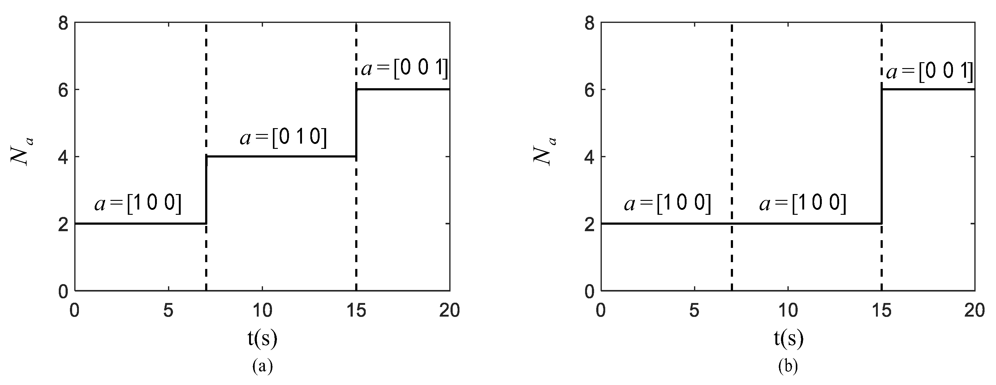
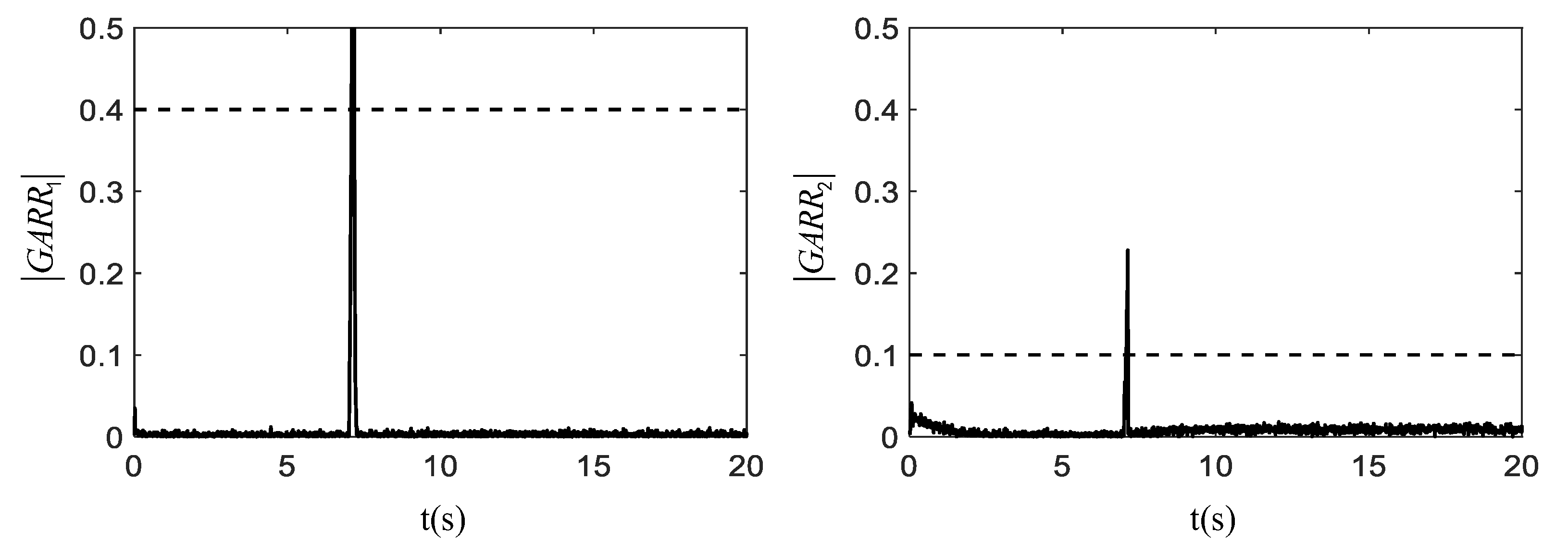
In the first fault scenario, the desired $N_a$ in operation and the actual $N_a$ in operation are shown in Figure 3, where the state of mode changes at 7 s and 15 s. The mode fault is set as $\left[100\right]$ between 7 s and 15 s, where the actual $N_a$ is 2 (while the desired $N_a$ is 4). Figure 4 illustrates the residual responses where all residuals exceed the thresholds (i.e., ${\iota }_1=0.4$ and ${\iota }_2=0.1$) at 7 s. After that, the condition monitoring system is enabled to check whether the inconsistency is due to a mode fault by comparing the CV = $\left[11\right]$ with the MCSM. Thus, $\left[100\right]$ and $\left[001\right]$ are two possible fault modes that may lead to the inconsistency. However, substituting $a=\left[001\right]$ into GARRs cannot make GARRs consistent. Therefore, the possible fault mode is $\left[100\right]$, and the GARRs will return within the threshold after a is set as $\left[100\right]$.

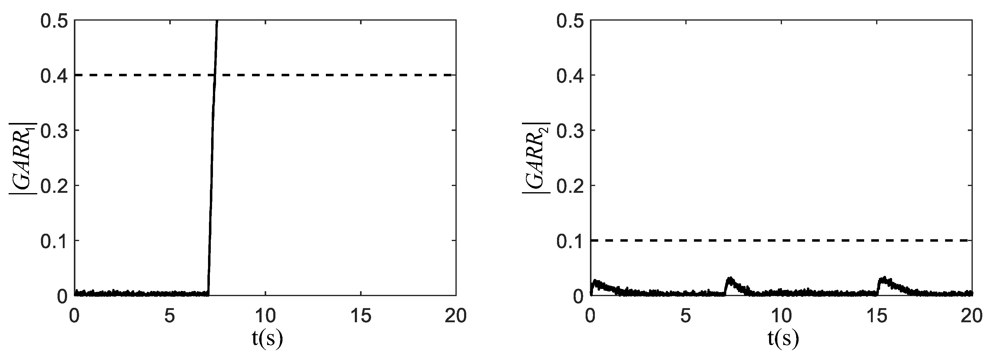
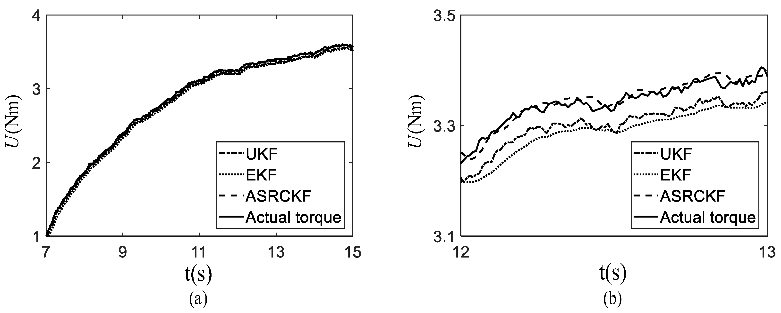
In the second fault scenario, the normal torque of the actuator is 1 Nm and an incipient fault of the actuator is injected at 7 s. The degradation law of incipient fault is defined as $U=1+0.9\times {\log }_2(t-t_0+1)+0.06\times B\left(t\right)$, where $t_0$ is 7 s and $B\left(t\right)$ is the Brownian motion which represents the randomness of degradation process. Figure 5 shows the responses of residuals by which the CV is $\left[10\right]$ after fault occurrence. As the nonzero CV has no matching in the MCSM, the possibility of mode fault is ruled out and SFC is obtained as $\left\{U,f_m,J_m\right\}$ by comparing CV with the FSM. To refine the SFC, the fault estimation module is activated by using the ASRCKF. Estimation results of $f_m$ and $J_m$ by ASRCKF are shown in Figure 6. According to estimation results, $f_m$ and $J_m$ are excluded from the SFC because their estimated values are close to the nominal ones. Figure 7a illustrates the estimated U where the estimated value significantly deviates from the nominal one. As a result, the true fault is U. To verify the superiority of ASRCKF, the EKF and UKF are also adopted to estimate U for comparison. Initial parameters for all filters are set as $P_0$ = diag(0.01,0.01,0.01,0.01,0.01,0.01,0.01), $Q_0$ = diag(0.1,0.1,0.1,0.1,0.1,0.1,0.1) and $R_0$ = diag(0.01,0.01).

In addition to the estimation result of U, the partial magnification of estimation results between 12 s and 13 s is illustrated in Figure 7b. To make the comparison quantitatively, the estimation performance of three methods is given in

Table 4. Comparison of fault estimation performance.

Algorithms	Mean Absolute Error	Mean Square Error
EKF	0.0591	0.0037
UKF	0.0366	0.0014
ASRCKF	0.0126	0.0009

, where ASRCKF is superior to other two algorithms due to the employment of the square root factor and the adaptive estimation of noise covariance matrixes.

After fault estimation, the estimation of the degradation model (i.e., the improved Wiener process) coefficients can be implemented using the estimated fault data of U. The estimate of $\beta$ using the least square method is shown in Figure 8a. It is observed that $MS{E}_{\beta }$ increases as $\beta$ increases, and $MS{E}_{\beta }$ reaches the minimum value when $\beta$ is equal to 2. Thus, the optimal value of $\beta$ is 2. In Figure 8b,c, the estimation results of $\alpha$ and $\sigma$ are obtained by the FKH. Initial parameters for KH and FKH are set as $l=25$, ${\mathrm{Y}}_{max}=150$, $M^{max}=0.01$, $V_f=0.02$, $D^{max}=0.005$, ${\zeta }_m=0.5$, and ${\zeta }_f=0.5$. Both KH and FKH run 10 times based on the same estimated fault data of U, and the comparison of estimation results is given in

Table 5. Comparison of degradation model coefficients estimation performance.

	KH	FKH
Mean of $\alpha$	0.8991	0.8993
Mean of $\sigma$	0.0595	0.0596
St.dev of $\alpha$	7.7463 ×${10}^{-5}$	7.4831 ×${10}^{-5}$
St.dev of $\sigma$	4.8988 ×${10}^{-5}$	4.5827 ×${10}^{-5}$
Mean iteration	72	60

. It can be observed from the table that KH and FKH could achieve similar estimation results. However, compared with KH, it is found that FKH is more efficient in terms of the convergence speed.

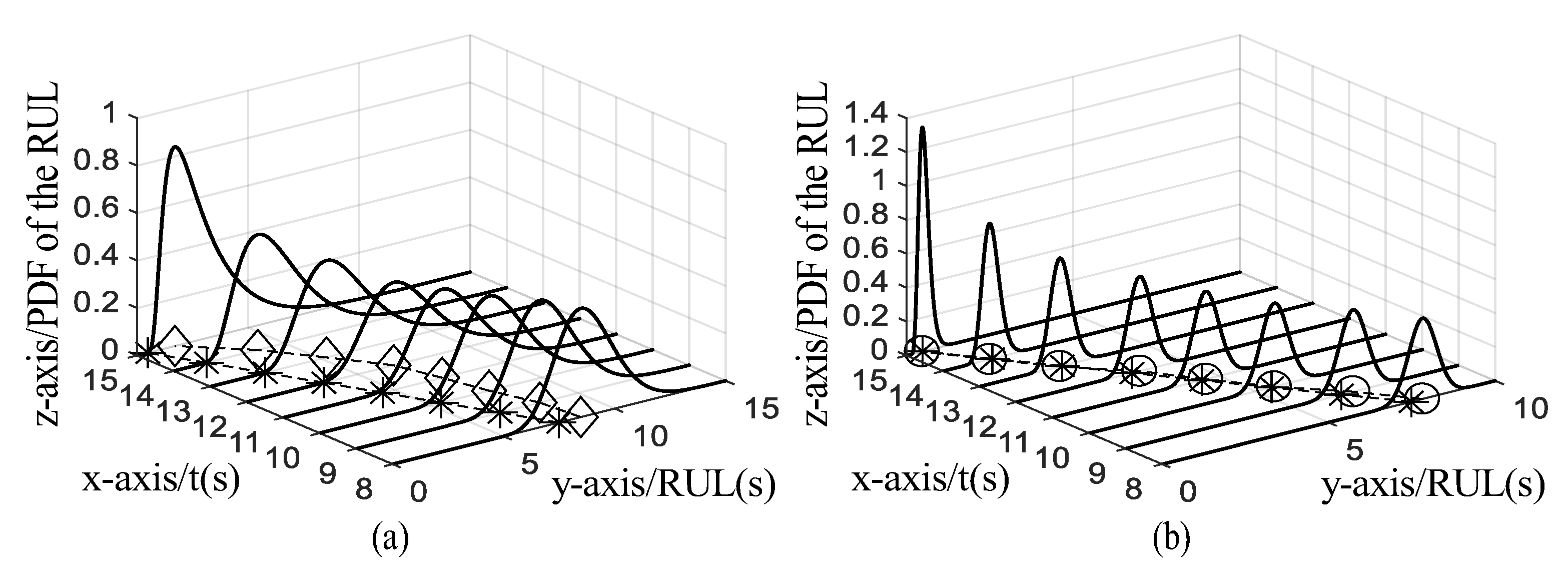
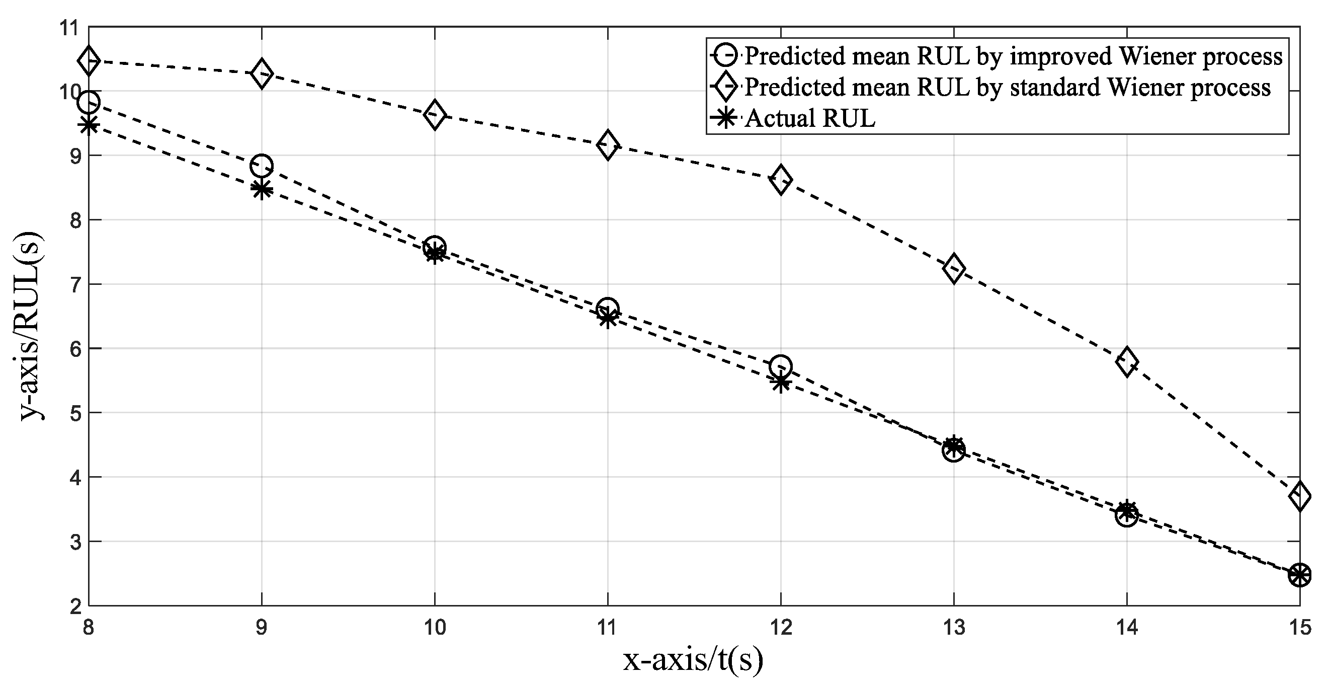
After the degradation model coefficients are obtained, RUL prediction can be carried out. The failure threshold of U is 4 Nm. Based on the estimated degradation model coefficients and (34), the PDF of RUL can be obtained. In Figure 9a, the x-axis, y-axis, and z-axis represent the time index, RUL, and the PDF of RUL. At each chosen instant, there is a curve (denoted by a solid line) covering different RULs. It is observed that actual RULs fall outside the coverage of the PDFs of RULs predicted by the standard Wiener process. The unsuccessful RUL prediction is due to the limited fitting capability of the standard Wiener process (i.e., only applicable to linear degradation process). In Figure 9b, the axes are set the same as in Figure 9a. It is found that the actual RULs are enveloped by the PDFs of RULs obtained by the improved Wiener process which is not the case for the standard Wiener process. For intuitive comparison, the top views of Figure 9a,b are combined to form Figure 10 where x-axis and y-axis still represent the time index and RUL. In Figure 10, the predicted mean RUL by standard Wiener process cannot track the actual RUL since only linear term is used. By contrast, the predicted mean RUL by improved Wiener process shows consistency with the corresponding actual RUL. Consequently, the proposed prognosis method using improved Wiener process performs better than the one using standard Wiener process.

6. Conclusions

In this article, a computational intelligence-based prognosis method is developed for the hybrid mechatronic system. Specifically, three main works are presented as follows (according to different sections): (1) GARRs derived by the DHBG are utilized to obtain MCSM and FSM, based on which both the unexpected mode changes and SFC can be isolated; (2) a novel filtering algorithm called ASRCKF is proposed for parameter estimation in the presence of unknown noise distributions. The ASRCKF functions better than other filtering methods (such as EKF and UKF); (3) the improved Wiener process incorporating nonlinear term is developed to capture the degradation of incipient fault, where the nonlinearity and randomness of degradation process are both taken into account. In addition, to ensure the accuracy of estimate, the FKH is proposed to estimate the degradation model coefficients efficiently.

In the future, there are three works that need to be addressed. First, only incipient fault is considered in this work. However, intermittent fault, abrupt fault, mode fault, or their combination may occur in the hybrid mechatronic system. Consequently, more sophisticated algorithms are required to handle this complicated fault situation. Second, the system is open-loop and no fault compensation is considered in this work. Thus, the fault-tolerant controller will be designed along with the effect of modeling and parametric uncertainties in the future work. Lastly, only simulation results are analyzed. Experiments will be carried out in modern industrial mechatronic systems to show practice significance of the proposed method.

References

1. Zhang, J.; Wang, H.; Zheng, J.; Cao, Z.; Man, Z.; Yu, M.; Chen, L. Adaptive sliding mode-based lateral stability control of steer-by-wire vehicles with experimental validations. IEEE Trans. Veh. Technol. 2020, 69, 9589–9600. [Google Scholar] [CrossRef]
2. Zhang, J.; Wang, H.; Ma, M.; Yu, M.; Yazdani, A.; Chen, L. Active front steering-based electronic stability control for steer-by-wire vehicles via terminal sliding mode and extreme learning machine. IEEE Trans. Veh. Technol. 2020, 69, 14713–14726. [Google Scholar] [CrossRef]
3. Zhou, D.; Zhao, Y.; Wang, Z.; He, X.; Gao, M. Review on diagnosis techniques for intermittent faults in dynamic systems. IEEE Trans. Ind. Electron. 2020, 67, 2337–2347. [Google Scholar] [CrossRef]
4. Prakash, O.; Samantaray, A.K.; Bhattacharyya, R. Model-based diagnosis of multiple faults in hybrid dynamical systems with dynamically updated parameters. IEEE Trans. Syst. Man Cybern.-Syst. 2017, 49, 1053–1072. [Google Scholar] [CrossRef]
5. Yu, M.; Wang, D.; Luo, M. Sequential prognosis of multiple failures for hybrid systems based on dynamic fault isolation and computational intelligence. In Proceedings of the 37th Annual Conference of the IEEE Industrial Electronics Society, Melbourne, VIC, Australia, 3 January 2012; pp. 2417–2422. [Google Scholar]
6. Zhao, F.; Koutsoukos, X.; Haussecker, H.; Reich, J.; Cheung, P. Monitoring and fault diagnosis of hybrid systems. IEEE Trans. Syst. Man Cybern. B Cybern. 2005, 35, 1225–1240. [Google Scholar] [CrossRef]
7. Cocquempot, V.; El Mezyani, T.; Staroswiecki, M. Fault detection and isolation for hybrid systems using structured parity residuals. In Proceedings of the 5th Asian Control Conference, Melbourne, VIC, Australia, 20–23 July 2004; pp. 1204–1212. [Google Scholar]
8. Xiao, C.; Yu, M.; Zhang, B.; Wang, H.; Jiang, C. Discrete component prognosis for hybrid systems under intermittent faults. IEEE Trans. Autom. Sci. Eng. 2020, 99, 1–12. [Google Scholar] [CrossRef]
9. Yu, M. Fault Diagnosis and Prognosis of Hybrid Systems Using Bond Graph Models and Computational Intelligence. Ph.D. Thesis, Nanyang Technological University, Singapore, 2012. [Google Scholar]
10. Yu, M.; Xiao, C.; Zhang, B. Event-triggered discrete component prognosis of hybrid systems using degradation model selection. IEEE Trans. Ind. Electron. 2021, 68, 11470–11481. [Google Scholar] [CrossRef]
11. Bhattacharyya, S.; Gebre-Egziabher, D. Kalman filter-based RAIM for GNSS receivers. IEEE Trans. Aerosp. Electron. Syst. 2015, 51, 2444–2459. [Google Scholar] [CrossRef]
12. Tudoroiu, N.; Khorasani, K. Satellite fault diagnosis using a bank of interacting Kalman filters. IEEE Trans. Aerosp. Electron. Syst. 2007, 43, 1334–1350. [Google Scholar] [CrossRef]
13. Söken, H.E.; Hajiyev, C. REKF and RUKF for pico satellite attitude estimation in the presence of measurement faults. J. Syst. Eng. Electron. 2014, 25, 288–297. [Google Scholar] [CrossRef]
14. Chang, L.; Hu, B.; Li, A.; Qin, F. Transformed unscented Kalman filter. IEEE Trans. Autom. Control 2013, 58, 252–257. [Google Scholar] [CrossRef]
15. Arasaratnam, I.; Haykin, S. Cubature Kalman filters. IEEE Trans. Autom. Control 2009, 54, 1254–1269. [Google Scholar] [CrossRef] [Green Version]
16. Chen, J.; Song, J.; Li, L.; Jia, G.; Ran, X.; Yang, C. UKF-based adaptive variable structure observer for vehicle sideslip with dynamic correction. IET Contr. Theory Appl. 2016, 10, 1641–1652. [Google Scholar] [CrossRef]
17. Yu, M.; Lu, H.; Wang, H.; Xiao, C.; Lan, D. Compound fault diagnosis and sequential prognosis for electric scooter with uncertainties. Actuators 2020, 9, 128. [Google Scholar] [CrossRef]
18. Lei, Y.; Li, N.; Gontarz, S.; Lin, J.; Radkowski, S.; Dybala, J. A model-based method for remaining useful life prediction of machinery. IEEE Trans. Reliab. 2016, 65, 1314–1326. [Google Scholar] [CrossRef]
19. Yang, B.; Liu, R.; Zio, E. Remaining useful life prediction based on a double-convolutional neural network architecture. IEEE Trans. Ind. Electron. 2012, 66, 9521–9530. [Google Scholar] [CrossRef]
20. Crowder, M.; Lawless, J. On a scheme for predictive maintenance. Eur. J. Oper. Res. 2007, 176, 1713–1722. [Google Scholar] [CrossRef]
21. Ye, Z.; Shen, Y.; Xie, M. Degradation-based burn-in with preventive maintenance. Eur. J. Oper. Res. 2012, 221, 360–367. [Google Scholar] [CrossRef]
22. Arogeti, S.A.; Wang, D.; Low, C.; Yu, M. Fault detection isolation and estimation in a vehicle steering system. IEEE Trans. Ind. Electron. 2012, 59, 4810–4820. [Google Scholar] [CrossRef]
23. Wang, Z.; Hu, C.; Fan, H. Real-time remaining useful life prediction for a nonlinear degrading system in service: Application to bearing data. IEEE-ASME Trans. Mechatron. 2018, 23, 211–222. [Google Scholar] [CrossRef]
24. Zhang, Z.; Si, X.; Hu, C.; Pecht, M.G. A prognostic model for stochastic degrading systems with state recovery: Application to Li-ion batteries. IEEE Trans. Reliab. 2017, 66, 1293–1308. [Google Scholar] [CrossRef]
25. Huh, J.; Hwa, J.; Seo, Y. Hierarchical system decomposition using genetic algorithm for future sustainable computing. Sustainability 2020, 12, 2177. [Google Scholar] [CrossRef] [Green Version]
26. Ju, Z.; Yang, L.; Yang, C.; Gegov, A.; Zhou, D. Advances in computational intelligence systems. Contributions presented at the 19th UK workshop on computational intelligence. Advances in intelligent systems and computing. In Proceedings of the 19th UK Workshop on Computational Intelligence, Portsmouth, UK, 4–6 September 2019. [Google Scholar]
27. Ruano, A.; Ge, S.S.; Guerra, T.M.; Lewis, F.L.; Principe, J.C.; Colnarič, M. Computational intelligence in control. Annu. Rev. Control 2014, 38, 233–242. [Google Scholar] [CrossRef]
28. Yang, J.; Zhao, Z.; Du, C.; Wang, W.; Peng, Q.; Qiu, J.; Wang, G. The realization of robotic neurorehabilitation in clinical: Use of computational intelligence and future prospects analysis. Expert Rev. Med. Devices 2020, 17, 1311–1322. [Google Scholar] [CrossRef]
29. Huh, J.; Seo, Y. Understanding edge computing: Engineering evolution with artificial intelligence. IEEE Access 2019, 7, 164229–164245. [Google Scholar] [CrossRef]
30. Gandomi, A.H.; Alavi, A.H. Krill herd: A new bio-inspired optimization algorithm. Commun. Nonlinear Sci. Numer. Simul. 2012, 17, 4831–4845. [Google Scholar] [CrossRef]
Figure 1. DHBG model of the hybrid mechatronic system.
Actuators 10 00213 g001
Figure 2. Block diagram of the developed prognosis method.
Actuators 10 00213 g002
Figure 3. N a : (a) Desired N a . (b) Actual N a .
Actuators 10 00213 g003
Figure 4. Responses of residuals in the first fault scenario.
Actuators 10 00213 g004
Figure 5. Responses of residuals in the second fault scenario.
Actuators 10 00213 g005
Figure 6. Estimation results: (a) Estimate of f m . (b) Estimate of J m .
Actuators 10 00213 g006
Figure 7. Estimation results: (a) Estimate of U. (b) Partial magnification of U estimate.
Actuators 10 00213 g007
Figure 8. Estimation results: (a) Estimate of β . (b) Estimate of α . (c) Estimate of σ .
Actuators 10 00213 g008
Figure 9. Predicted PDFs of RULs: (a) PDF of RUL obtained by standard Wiener process. (b) PDF of RUL obtained by improved Wiener process. (“⋄”: predicted mean RUL by standard Wiener process; “*”: actual RUL; “◯”: predicted mean RUL by improved Wiener process).
Actuators 10 00213 g009
Figure 10. Mean RUL prediction results.
Actuators 10 00213 g010