
H∞ Reliable Dynamic Output-Feedback Controller Design for Discrete-Time Singular Systems with Sensor Saturation


Abstract
:1. Introduction
- it is attractive because the analysis of the controller is conducted for systems operating in real circumstances with exogenous disturbances, stochastic actuator failures, and sensor saturations,
- the proposed control scheme should be reliable and can accommodate the actuator failures and the sensor nonlinearities,
- without any model transformation or matrix decomposition, the controller design is carried out by introducing a slack variable to obtain a strict LMI condition,
- the resulting closed-loop system is able to attenuate the perturbations effects in the H∞ sense.
2. Problem Formulation and Preliminaries
- matrix may be singular, with rank;
- system state is not available for measurement, is stabilizable, and is detectable;
- saturation function is defined aswith , where is the i-th element of the saturation level vector .
- 1.
- Pair is said to be regular, if is not identically zero for each ;
- 2.
- Pair is said to be causal if for each ;
- 3.
- System (1) is said to be stochastically stable, if for any initial state , the condition is satisfied;
- 4.
- System (1) is said to be stochastically admissible, if it is regular, causal, and stochastically stable.
3. H∞ Performance and Admissibility Analysis
4. H∞ Controller Design
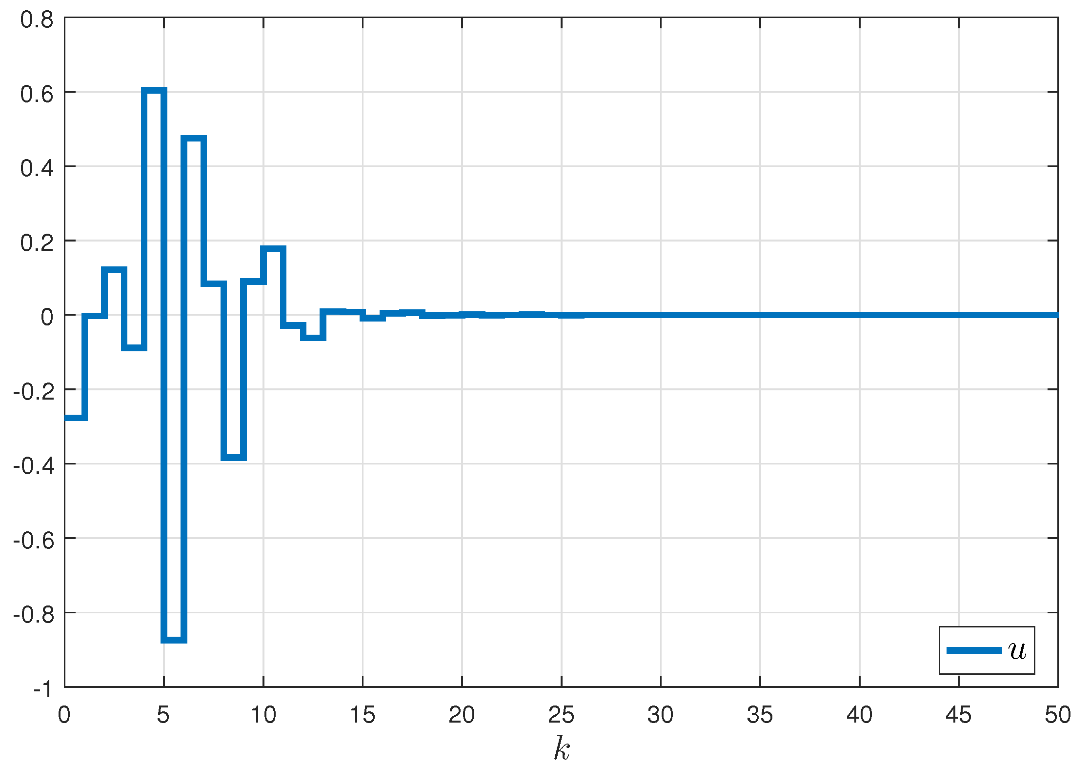
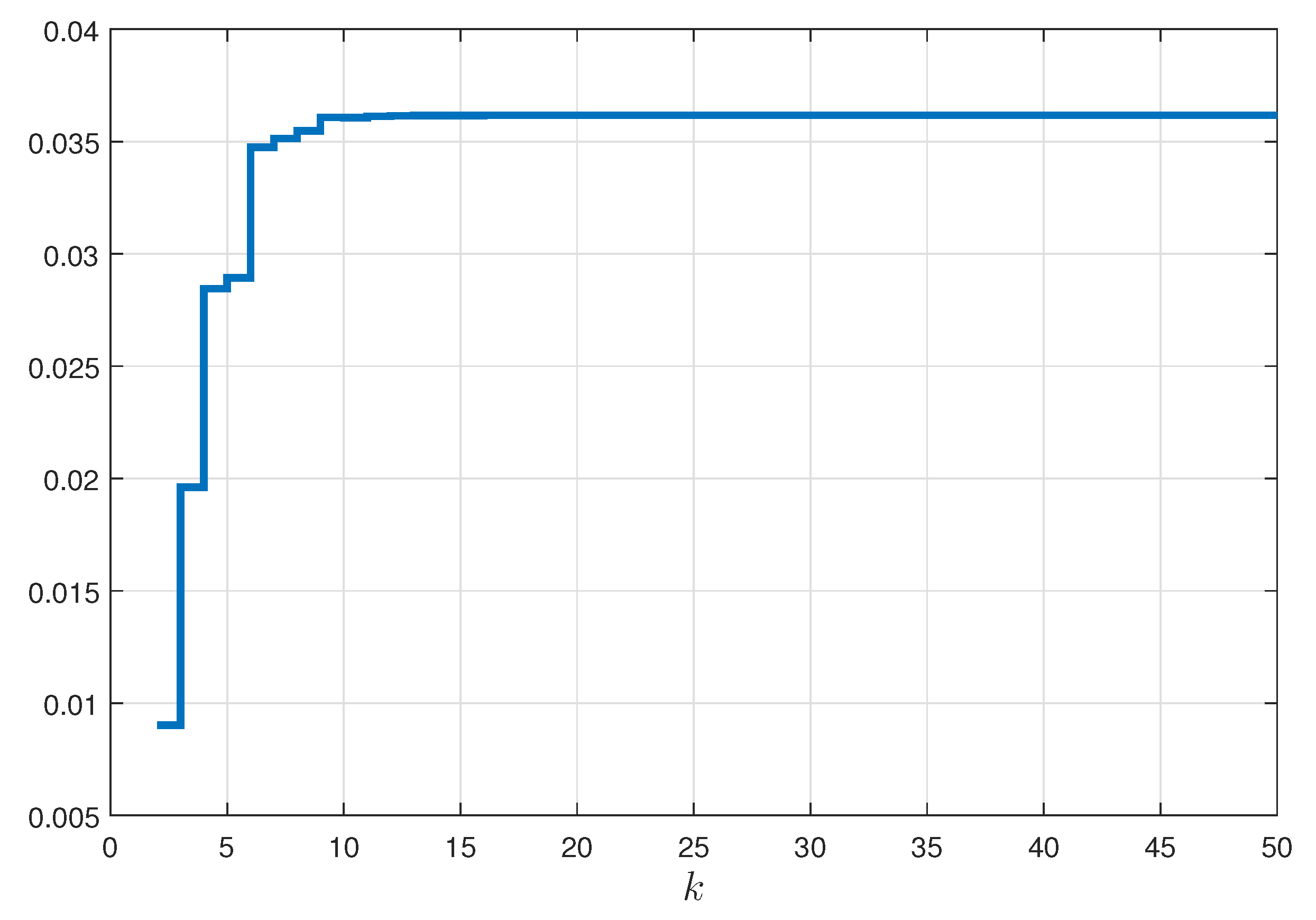
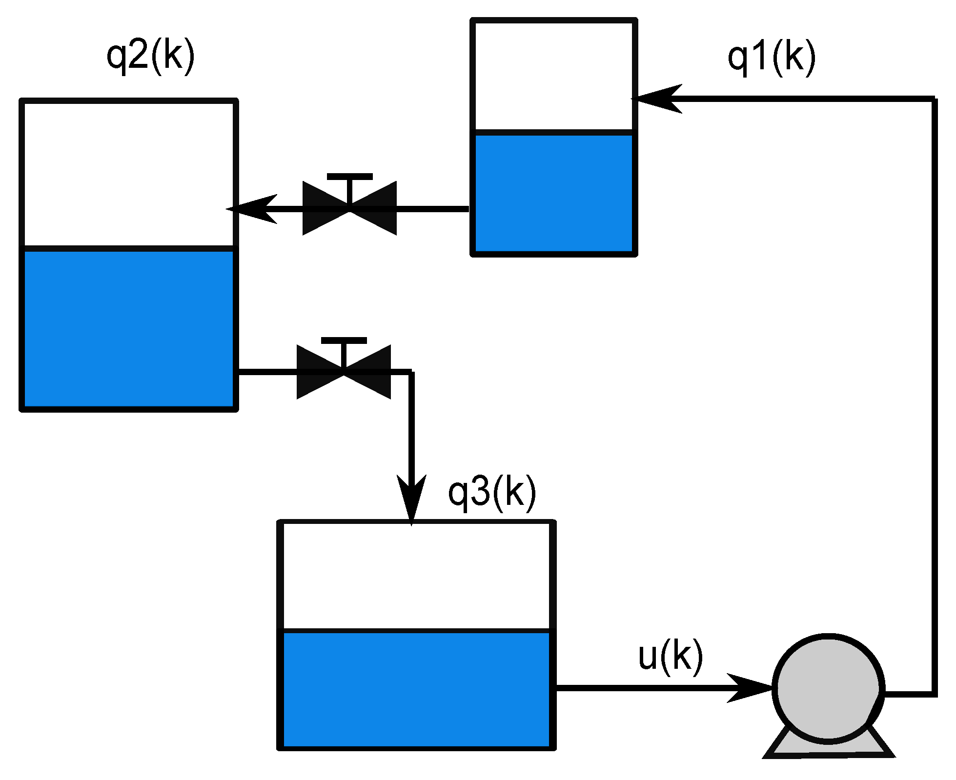
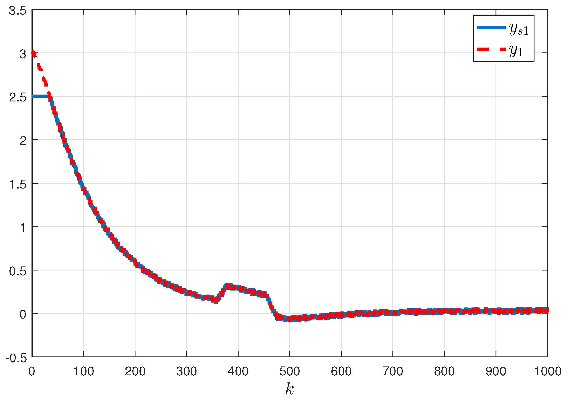
5. Numerical Examples
6. Conclusions
Author Contributions
Funding
Conflicts of Interest
References
- Cao, Y.Y.; Lin, Z.; Chen, B. An Output Feedback H∞ Controller Design for Linear Systems Subject to Sensor Nonlinearities. IEEE Trans. Circuits Syst. Fundam. Theory Appl. 2003, 50–57, 914–921. [Google Scholar]
- Zuo, Z.; Wang, J.; Huang, L. Output feedback H∞ controller design for linear discrete-time systems with sensor nonlinearities. IEE Proc. Control Theory Appl. 2005, 152, 19–26. [Google Scholar] [CrossRef]
- Rubio, J.D.J.; Lughofer, E.; Pieper, J.; Cruz, P.; Martinez, D.I.; Ochoa, G.; Islas, M.A.; Garcia, E. Adapting H∞ controller for the desired reference tracking of the sphere position in the maglev process. Inf. Sci. 2021, 569, 669–686. [Google Scholar] [CrossRef]
- Martinez, D.I.; Rubio, J.D.; Garcia, V.; Vargas, T.M.; Islas, M.A.; Pacheco, J.; Gutierrez, G.J.; Meda-Campaña, J.A.; Mujica-Vargas, D.; Aguilar-Ibañez, C. Transformed Structural Properties Method to Determine the Controllability and Observability of Robots. Appl. Sci. 2021, 11, 3082. [Google Scholar] [CrossRef]
- Escobedo-Alva, J.O.; García-Estrada, E.C.; Páramo-Carranza, L.A.; Meda-Campaña, J.A.; Tapia-Herrera, R. Theoretical Application of a Hybrid Observer on Altitude Tracking of Quadrotor Losing GPS Signal. IEEE Access 2018, 6, 76900–76908. [Google Scholar] [CrossRef]
- Soriano, L.A.; Zamora, E.; Vazquez-Nicolas, J.M.; Hernández, G.; Barraza Madrigal, J.A.; Balderas, D. PD Control Compensation Based on a Cascade Neural Network Applied to a Robot Manipulator. Front. Neurorobot. 2020, 14, 78. [Google Scholar] [CrossRef]
- Zhang, D.; Zhou, Z.; Jia, X. Networked fuzzy output feedback control for discrete-time Takagi-Sugeno fuzzy systems with sensor saturation and measurement noise. Inf. Sci. 2018, 457–458, 182–194. [Google Scholar] [CrossRef]
- Duan, R.; Li, J. Finite-time distributed H∞ filtering for Takagi-Sugeno fuzzy system with uncertain probability sensor saturation under switching network topology: Non-PDC approach. Appl. Math. Comput. 2020, 371, 1–21. [Google Scholar] [CrossRef]
- Liu, Y.; Ma, Y.; Wang, Y. Reliable sliding mode finite-time control for discrete-time singular Markovian jump systems with sensor fault and randomly occurring nonlinearities. Int. J. Robust Nonlinear Control 2018, 28, 381–402. [Google Scholar] [CrossRef]
- Tao, Y.; Shen, D.; Wang, Y.; Ye, Y. Reliable H∞ control for uncertain nonlinear discrete-time systems subject to multiple intermittent faultsin sensors and/or actuators. J. Frankl. Inst. 2015, 352, 4721–4740. [Google Scholar] [CrossRef]
- Qiu, J.; Wei, Y.; Karimi, H.R.; Gao, H. Reliable control of discrete-time piecewise-affine time-delay systems via output feedback. IEEE Trans. Reliab. 2018, 67, 79–91. [Google Scholar] [CrossRef]
- Wang, Y.; Shi, P.; Yan, H. Reliable control of fuzzy singularly perturbed systems and its application to electronic circuits. IEEE Trans. Circuits Syst. I 2018, 65, 3519–3528. [Google Scholar] [CrossRef]
- Wang, Y.; Yang, X.; Yan, H. Reliable Fuzzy Tracking Control of Near-Space Hypersonic Vehicle Using Aperiodic Measurement Information. IEEE Trans. Ind. Electron. 2019, 66, 9439–9447. [Google Scholar] [CrossRef]
- Xu, S.; Lam, J.; Zou, Y. H∞ filtering for singular systems. IEEE Trans. Autom. Control 2003, 48, 2217–2222. [Google Scholar]
- Feng, J.; Cui, P.; Cheng, Z. H∞ output feedback control for descriptor systems with delayed states. J. Control Theory Appl. 2005, 4, 342–347. [Google Scholar] [CrossRef]
- Boukas, E. Singular linear systems with delay: H∞ stabilization. Optim. Control Appl. Methods 2007, 28, 259–274. [Google Scholar] [CrossRef]
- Dai, L. Singular Control Systems. In Lecture Notes in Control and Information Sciences; Springer: New York, NY, USA, 1989; Volume 118. [Google Scholar]
- Duan, G. Analysis and Design of Descriptor Linear Systems; Springer: New York, NY, USA, 2010. [Google Scholar]
- Kchaou, M. Robust observer-based sliding mode control for nonlinear uncertain singular systems with time-varying delay and input non-linearity. Eur. J. Control 2019, 49, 15–25. [Google Scholar] [CrossRef]
- Liu, Y.; Ma, Y.; Wang, Y. Reliable finite-time sliding-mode control for singular time-delay system with sensor faults and randomly occurring nonlinearities. Appl. Math. Comput. 2018, 320, 341–357. [Google Scholar] [CrossRef]
- Li, M.; Chen, X.; Liu, M.; Zhang, Y.; Zhang, H. Asynchronous Adaptive Fault-Tolerant Sliding-Mode Control for T-S Fuzzy Singular Markovian Jump Systems with Uncertain Transition Rates. IEEE Trans. Cybern. 2020. [Google Scholar] [CrossRef]
- Jun, H.; Cui, Y.; Lv, C.; Chen, D.; Zhang, H. Robust adaptive sliding mode control for discrete singular systems with randomly occurring mixed time-delays under uncertain occurrence probabilities. Int. J. Syst. Sci. 2020, 51, 987–1006. [Google Scholar]
- Ma, S.; Cheng, Z.; Zhang, C. Delay-dependent robust stability and stabilisation for uncertain discrete singular systems with time-varying delays. IET Control Theory Appl. 2007, 1, 1086–1095. [Google Scholar] [CrossRef]
- Fang, M. Delay-dependent stability analysis for discrete singular systems with time-varying delays. Acta Autom. Sin. 2010, 36, 751–755. [Google Scholar] [CrossRef]
- Feng, Z.; Li, W.; Lam, J. New admissibility analysis for discrete singular systems with time-varying delay. Appl. Math. Comput. 2015, 265, 1058–1066. [Google Scholar] [CrossRef]
- Regaieg, M.A.; Kchaou, M.; El Hajjaji, A.; Chaabane, M. Robust H∞ guaranteed cost control for discrete-time switched singular systems with time-varying delay. Optim. Control Appl. Methods 2019, 40, 119–140. [Google Scholar] [CrossRef]
- Ma, Y.; Jia, X.; Zhang, Q. Robust finite-time non-fragile memory H∞ control for discrete-time singular Markovian jumping systems subject to actuator saturation. J. Frankl. Inst. 2017, 354, 8256–8282. [Google Scholar] [CrossRef]
- Li, F.; Xu, S.; Zhang, B. Resilient Asynchronous H∞ Control for Discrete-Time Markov Jump Singularly Perturbed Systems Based on Hidden Markov Model. IEEE Trans. Syst. Man Cybern. Syst. 2020, 50, 2860–2869. [Google Scholar] [CrossRef]
- Kchaou, M.; Jerbi, H.; Abassi, R.; VijiPriya, J.; Hmidi, F.; Kouzou, A. Passivity-based asynchronous fault-tolerant control for nonlinear discrete-time singular markovian jump systems: A sliding-mode approach. Eur. J. Control 2021, 60, 95–113. [Google Scholar] [CrossRef]
- Kwon, N.K.; Park, I.S.; Park, P.; Park, C. Dynamic Output-Feedback Control for Singular Markovian Jump System: LMI Approach. IEEE Trans. Autom. Control 2017, 62, 5396–5400. [Google Scholar] [CrossRef]
- Long, S.; Zhong, S. H∞ control for a class of discrete-time singular systems via dynamic feedback controller. Appl. Math. Lett. 2016, 58, 110–118. [Google Scholar] [CrossRef]
- Zhang, J.; Ma, S. Robust H∞ indefinite guaranteed cost dynamic output feedback control of singular semi-Markov jump systems. J. Frankl. Inst. 2021. [Google Scholar] [CrossRef]
- Park, I.S.; Park, C.; Kwon, N.K.; Park, P. Dynamic output-feedback control for singular interval-valued fuzzy systems: Linear matrix inequality approach. Inf. Sci. 2021, 576, 393–406. [Google Scholar] [CrossRef]
- Wu, Z.G.; Park, J.; Su, H.; Chu, J. Stochastic stability analysis for discrete-time singular Markov jump systems with time-varying delay and piecewise-constant transition probabilities. J. Frankl. Inst. 2012, 349, 2889–2902. [Google Scholar] [CrossRef]
- Ma, Y.; Jia, X.; Liu, D. Finite-time dissipative control for singular discrete-time Markovian jump systems with actuator saturation and partly unknown transition rates. Appl. Math. Model. 2018, 53, 49–70. [Google Scholar] [CrossRef]
- Wang, Z.; Ho, D.W.; Dong, H.; Gao, H. Robust H∞ Finite-Horizon Control for a Class of Stochastic Nonlinear Time-Varying Systems Subject to Sensor and Actuator Saturations. IEEE Trans. Autom. Control 2010, 55, 1716–1723. [Google Scholar]
- Hu, J.; Wang, Z.; Gao, H.; Stergioulas, L.K. Probability-guaranteed H∞ finite-horizon filtering for a class of nonlinear time-varying systems with sensor saturations. Syst. Control Lett. 2012, 64, 477–484. [Google Scholar] [CrossRef] [Green Version]
- Khalil, H. Nonlinear Systems; Prentice-Hall: Upper Saddle River, NJ, USA, 1996. [Google Scholar]
- Li, Z.; Mobin, M.; Keyser, T. Multi-objective and multi-stage reliability growth planning in early product development stage. IEEE Trans. Reliab. 2015, 65, 769–781. [Google Scholar] [CrossRef]
- Xu, S.; Lam, J. Robust Control and Filtering of Singular Systems; Springer: Berlin/Heidelberg, Germany, 2006. [Google Scholar]
- Ma, S.; Boukas, E. Robust H∞ filtering for uncertain discrete Markov jump singular systems with mode-dependent time delay. IET Control Theory Appl. 2009, 3, 351–361. [Google Scholar] [CrossRef]
- Peterson, I. A stabilization algorithm for a class uncertain linear systems. Syst. Control Lett. 1987, 8, 351–357. [Google Scholar] [CrossRef]
- Saadni, S.; Chaabane, M.; Mehdi, D. Robust stability and stabilization of a class of singular systems with multiple time-varying delays. Asian J. Control 2006, 8, 1–11. [Google Scholar] [CrossRef]
- Chadli, M.; Darouach, M. Novel bounded real lemma for discrete-time descriptor systems: Application to H∞ control design. Automatica 2012, 2012, 449–453. [Google Scholar] [CrossRef]
- Chadli, M.; Darouach, M. Further enhancement on robust control design for discrete-time singular systems. IEEE Trans. Autom. Control 2014, 59, 494–500. [Google Scholar] [CrossRef] [Green Version]
- Wang, W.; Ma, S.; Zhang, C. Stability and Static Output Feedback Stabilization for a Class of Nonlinear Discrete-Time Singular Switched Systems. Int. J. Control Autom. Syst. 2013, 11, 1138–1148. [Google Scholar] [CrossRef]
- Ji, X.; Su, H.; Chu, J. Robust state feedback H∞ control for uncertain linear discrete singular systems. IET Control Theory Appl. 2007, 1, 195–200. [Google Scholar] [CrossRef]
- Belov, A.A.; Andrianova, O.G.; Kurdyukov, A. Control of Discrete-Time Descriptor Systems: An Anisotropy-Based Approach; Springer: Cham, Switzerland, 2018. [Google Scholar]


| Methods | |
|---|---|
| Theorem 2 | (44) |
| Theorem 2 in [31] | Infeasible |
| Theorem 3 in [47] | Infeasible |
| Theorem 7 in [44] | Infeasible |
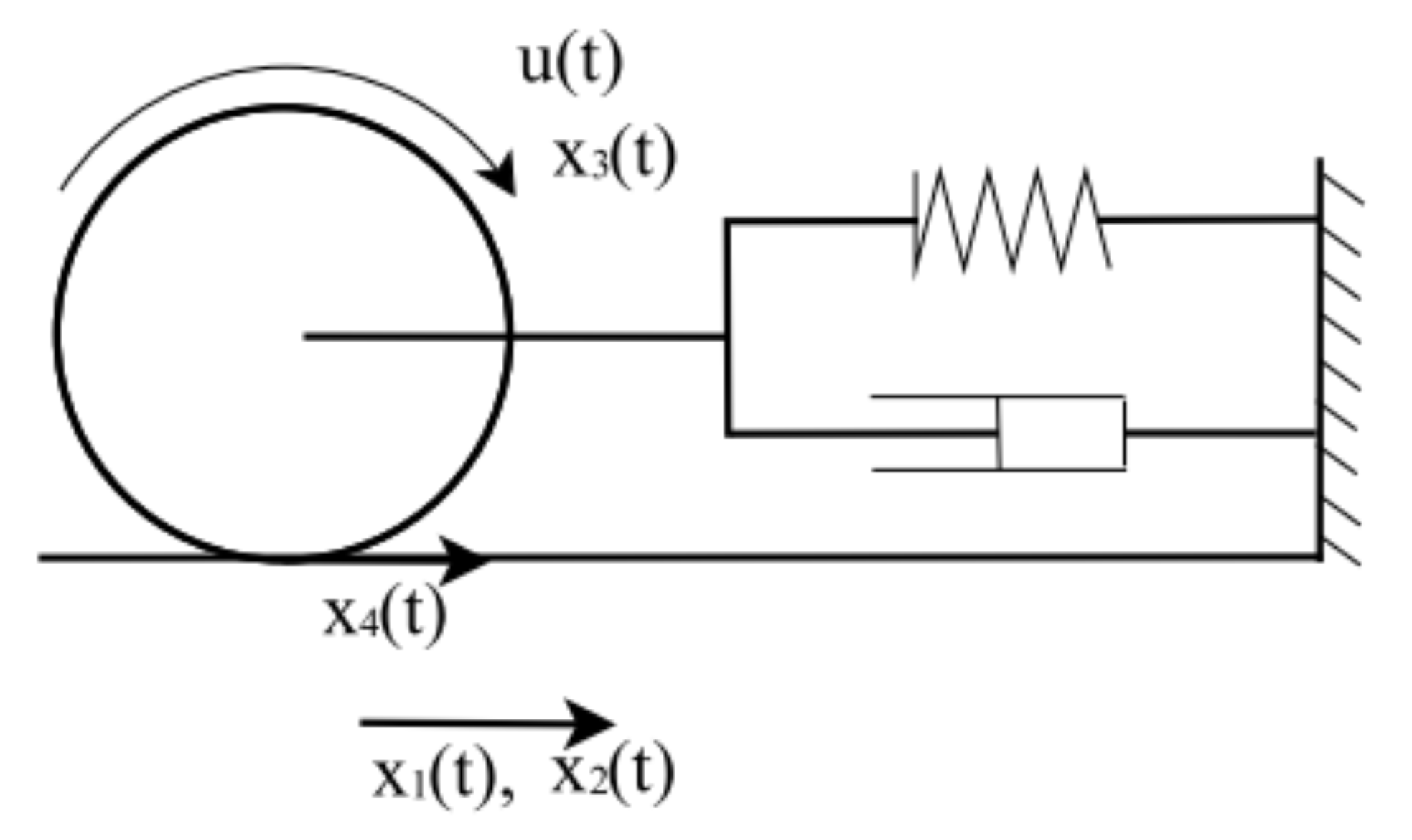
| Parameter | Value | Unit |
|---|---|---|
| K | 100 | [] |
| b | 30 | [Ns/m] |
| m | 40 | [kg] |
| J | [] | |
| r | 10 | [cm] |
Publisher’s Note: MDPI stays neutral with regard to jurisdictional claims in published maps and institutional affiliations. |
© 2021 by the authors. Licensee MDPI, Basel, Switzerland. This article is an open access article distributed under the terms and conditions of the Creative Commons Attribution (CC BY) license (https://creativecommons.org/licenses/by/4.0/).
Share and Cite
Kchaou, M.; Jerbi, H.; Ali, N.B.; Alsaif, H. H∞ Reliable Dynamic Output-Feedback Controller Design for Discrete-Time Singular Systems with Sensor Saturation. Actuators 2021, 10, 196. https://doi.org/10.3390/act10080196
Kchaou M, Jerbi H, Ali NB, Alsaif H. H∞ Reliable Dynamic Output-Feedback Controller Design for Discrete-Time Singular Systems with Sensor Saturation. Actuators. 2021; 10(8):196. https://doi.org/10.3390/act10080196
Chicago/Turabian StyleKchaou, Mourad, Houssem Jerbi, Naim Ben Ali, and Haitham Alsaif. 2021. "H∞ Reliable Dynamic Output-Feedback Controller Design for Discrete-Time Singular Systems with Sensor Saturation" Actuators 10, no. 8: 196. https://doi.org/10.3390/act10080196
APA StyleKchaou, M., Jerbi, H., Ali, N. B., & Alsaif, H. (2021). H∞ Reliable Dynamic Output-Feedback Controller Design for Discrete-Time Singular Systems with Sensor Saturation. Actuators, 10(8), 196. https://doi.org/10.3390/act10080196