Control of a Rehabilitation Robotic Device Driven by Antagonistic Soft Actuators

Abstract

Stroke is becoming a widely concerned social problem, and robot-assisted devices have made considerable contributions in the training and treatment of rehabilitation. Due to the compliance and continuous deformation capacity, rehabilitation devices driven by soft actuators are attached to widespread attention. Considering the large output force of pneumatic artificial muscle (PAM) and the biological musculoskeletal structure, an antagonistic PAM-driven rehabilitation robotic device is developed. To fulfill the need for control of the proposed device, a knowledge-guided data-driven modeling approach is used and an adaptive feedforward–feedback control approach is presented to ensure the motion accuracy under large deformation motion with high frequency. Finally, several simulations and experiments are carried out to evaluate the performance of the developed system, and the results show that the developed system with the proposed controller can achieve expected control performance under various operations.

1. Introduction

Stroke, a disease caused by the insufficient blood supply to the brain due to blockage or sudden rupture of blood vessels, is becoming a leading cause of mortality and disability. The World Health Organization (WHO) describes stroke as “rapidly developing clinical signs of focal (or global) disturbance of cerebral function, with symptoms lasting 24 h or longer or leading to death, with no apparent cause other than of vascular origin” [1]. According to medical reports, stroke has been the second largest cause of death globally after ischemic heart disease, and up to now, the burden of the stroke remains heavy [2].

As a troubling disease, stroke usually causes a loss of physical strength on one side of the body, paralysis or hemiplegia. More than $2/3$ patients affected by stroke suffer from impaired upper limb motor function, which brings great inconvenience to daily life [3]. Medical studies have found that an efficient way to treat stroke is the timely rehabilitation training. Moreover, many trials have shown that task-specific, high-intensity exercises in an active, functional, and highly repetitive manner can enhance motor recovery [4]. However, the traditional exercise therapy performed by the therapists is always tedious and inefficient [5]. To assist patients in accurately, quantitatively and personally completing the therapy, rehabilitation robotic devices are being widely adopted recently.

Most of the rehabilitation robotic devices are actuated by “hard” actuators such as electric motors. These kinds of actuators are able to provide sufficient power and accurate motion. However, limitations such as heavy weight and confined motion direction restrict their usage in rehabilitation. Soft actuators, in contrast, have better biomimetic qualities due to their compliance and flexibility.

Many soft actuators for robotic applications have been investigated, such as pneumatic artificial muscle (PAM) [6,7,8], shape memory actuators (SMA) [9,10], dielectric elastomer actuators (DEA) [11,12] and soft fluidic actuators (SFA) [13,14,15]. Similar to biological muscles, once stimulated, these soft actuators can arise deformation responses such as stretching, bending, tightening, or expanding. Hence, these soft actuators are generally compatible with robotic applications involving human body interaction. Among the actuators explored above, PAMs stand out in rehabilitation robotic applications [16], because PAMs possess high power-to-weight ratios and prominent inherent compliance [17]. Moreover, compared with other aforementioned soft actuators, PAMs are able to generate a greatly larger output force. Thus, many rehabilitation robotic devices actuated by PAMs have been developed. The notable examples include RUPERT [18,19,20] and ARMin [21,22,23].

Although the PAMs adopted in the aforementioned robotic devices exhibited muscle-like motion in a rehabilitation process, control of these robotic devices still remains a huge challenge. In the exercise training process, due to the nonlinearity, viscoelasticity, and time-dependent properties of soft materials, precision motion control of a PAM-driven robotic device in large deformation motion with high frequency, which is normally necessary for rehabilitation, is very difficult. Previously, a lot of studies have been conducted to improve the robustness control system of PAMs-driven robotic devices, such as a basic proportional–integral–derivative (PID) control approach proposed in [24]. A modified sliding mode control (SMC) approach [25], an adaptive fuzzy logic control (FLC) approach [26] and an adaptive recurrent neural networks (ARNN) control approach [27] were proposed to handle the nonlinearity problem of the system. However, all these control schemes mentioned above are suitable with low-frequency motion, and few of these approaches can be applied to robotic applications in practice under large deformation with fast response.

Biologically, due to the similarities between PAM and biological muscle, as well as the purpose of assisting patients, an intuitive solution for the design of rehabilitation robots’ structure and control system is to mimic the biological system. Most motions of living beings are driven by the muscles in antagonistic pairs, thus one objective of this paper is to investigate the control issues of PAMs in antagonistic pairs. Actually, antagonistic PAMs have been extensively studied, such as the study presented in [28]. However, none of them were designed entirely referring to biology as biceps and triceps. The main purpose of adopting antagonistic pairs is to generate bidirectional actuation and make up for the deficiency of passive recovery characteristics.

Further on, referring to the biological neural control mechanisms, a controller inspired by the cerebellar computing mechanism called cerebellar model articulation controller (CMAC) is adopted in this paper. The CMAC is a kind of adaptive neural network for approximating complex nonlinear functions. It is essentially a technology for nonlinear function mapping, which is a feedforward network virtually. Due to its local learning strategy, CMAC can improve the learning speed while ensuring the approximation performance with the nonlinear functions. Furthermore, CMAC is suitable for continuous input space and is not sensitive to the order of given data as well. Therefore, CMAC is widely used in real-time control of the nonlinear system under complex dynamic conditions [29,30].

This work mainly aims to design a rehabilitation robotic device that can be equipped on the upper limb for stroke patients under an accurate control. The main contributions of this study are listed as follows: (i) Drawing from the biological system, antagonistic pairs in the bio-inspired structure are designed to overcome the uncontrollable passive recovery characteristic, which mimic the coupling relationship of living beings’ antagonist muscles. In this structure, the system is able to achieve bidirectional actuation, and the motion can be more compliant with human dynamics. (ii) A knowledge-guided data-driven modeling approach by using the spring–dashpot model is employed to simplify the difficulties in the modeling process, where the model parameters will be determined via system identification. (iii) To achieve good control performance, an adaptive feedforward–feedback controller consisting of a PID controller and a CMAC is proposed, which can perform well in shortening the response time and improving the motion accuracy. Significantly, the effect of CMAC is corresponding to the cerebellum in human beings, and the PID controller is used as error-based feedback control.

The rest of this paper is organized as follows. The design of the robot prototype with the kinematics and dynamics analysis is presented in Section 2. Next, the dynamic models of the PAM, as well as the antagonistic pairs, are established in Section 3. In Section 4, the adaptive feedforward–feedback control scheme is designed and analyzed. Next, both simulations and experiments are carried out to verify and validate the feasibility of the developed robot system in Section 5. Finally, Section 6 gives the conclusions.

2. Robotic Device

In this section, the mechanical structure and its working principle are explained, and then its kinematics and dynamics analysis is given.

2.1. Rehabilitation-Arm Design

Usually, muscles in biological systems are placed in antagonistic pairs, which are more flexible and faster in accomplishing assigned tasks compared with a single muscle.

Figure 1a shows three common antagonistic configurations, which are pulley type, lever type and pendulum type, respectively. Each type of configuration has its own characteristics, and they have been widely used in engineering practice. However, when looking for the optimal solution from biological systems, a different configuration illustrated in Figure 1b is found. Inspired by this configuration, the structure for the rehabilitation pneumatic robotic arm is designed. Thus, a robot manipulator shown in Figure 1c is developed in this paper.

The motivations of adopting this bio-inspired structure are: (i) The robot manipulator is designed for stroke patients’ rehabilitation, this structure is similar to physiological structure of human arms. It could mobilize the muscle groups of the arm to a greater extent in principle, and thus it is able to achieve better rehabilitation results. (ii) Unlike conventional antagonistic pairs, in this paper, the soft and deformable actuators can achieve antagonistic effect even if there is a distortion during transmission, which is able to obtain good operational feasibility in practice.

2.2. Kinematics and Dynamics Analysis

Figure 2a shows the physical structure of the robot manipulator. As can be seen, two McKibben PAMs are combined with an artificial skeleton (consisting of an upper arm and a forearm) through four connection points.

For the sake of illustration, the upper arm is defined as $B1$ while the forearm as $B2$. As mentioned above, the McKibben PAM $P1$ represents the biceps and $P2$ represents the triceps. Then, $P1$ and $B1$ are connected at $N_1$, $P1$ and $B2$ are connected at $N_2$, $P2$ and $B1$ are connected at $N_4$, and $P2$ and $B2$ are connected at $N_3$. The distances between the endpoints of $P1/P2$ and the corresponding connection points are defined as $d_1$, $d_2$, $d_3$, $d_4$.

In the initial state shown in Figure 2b, $P1$ is divided into two sections with the center of the elbow joint (rotation axis) as the reference, the lengths of these two sections are noted as $d_5$, $d_6$. Similarly, $d_7$, $d_8$ could be obtained with $P2$. Define the length of $P1$ as $L_1$ and the length of $P2$ as $L_2$, then the initial lengths of PAMs can be expressed as

$$\left\{\begin{array}{c}{L}_{10}=d_5+d_6\hfill \\ L_{20}=d_7+d_8\hfill \end{array}\right..$$

(1)

When the robot manipulator rotates to an angle of $\theta$ as shown in Figure 2c, it can be seen obviously that both PAMs are deformed to different angles. According to geometric principles, the kinematics can be obtained. Firstly, the relationship between the length of $P2$ and the rotation angle $\theta$ can be simply expressed as

$$L_2=d_7+d_8+d_3\theta .$$

(2)

The length of $P1$ can be obtained through the Pythagorean theorem:

$$\left\{\begin{array}{c}{L}_{11}=d_6-(d_{1}sin\theta -d_{5}cos\theta )\hfill \\ L_{12}=d_{1}cos\theta +d_{5}sin\theta -d_2\hfill \\ L_1=\sqrt{L_{11}^2+L_{12}^2}\hfill \end{array}\right..$$

(3)

Since the human arm is naturally drooping, the rotational moment of the forearm is considered as

$$\begin{array}{cc}\hfill M& =F_1{l}_{F_1}-F_2{l}_{F_2}+M_G\hfill \\ \hfill & =F_1{l}_F-F_2{d}_3-mg{l}_{O_G}\sin (\theta +\beta ),\hfill \end{array}$$

(4)

where $F_1$ and $F_2$ represent the force driven by $P1$ and $P2$, respectively, $l_{F_1}$ and $l_{F_2}$ are the corresponding moment arm. $M_G$ is the representation of the gravitational moment, and $l_F$ is the vertical distance between the force direction $\overrightarrow{F_1}$ and the forearm $B2$. $l_{O_G}$ is the distance between O and $O_G$ shown in Figure 2b. According to the Law of Cosines, $l_F$ can be obtained from the following equation

$$\left\{\begin{array}{c}a=\sqrt{d_1^2+d_5^2}\hfill \\ b=\sqrt{d_2^2+d_6^2}\hfill \\ \alpha =\pi -arctan\frac{d_1}{d_5}-arctan\frac{d_2}{d_6}-\theta \hfill \\ l_f=\frac{ab{L}_{1}sin\alpha }{a^2+b^2-2abcos\alpha }=\frac{absin\alpha }{L_1}\hfill \end{array}\right..$$

(5)

In addition, the dynamic model derived via Euler–Lagrange equation for this robot manipulator is

$$\tau =J\ddot{\theta }+C\dot{\theta }+G\left(\theta \right),$$

(6)

where J is the inertia coefficient, C is the damping coefficient and $G\left(\theta \right)$ is the gravitational torque.

Thus, the following equation can be derived

$$J\ddot{\theta }=F_1{l}_F-F_2{d}_3+\chi (\theta ,\dot{\theta }),$$

(7)

where $J(\theta ,\dot{\theta })$ includes the torque caused by gravity and other external disturbances.

3. System Modeling

Modeling is important for the control scheme design [31,32]. In this section, the system modeling of the PAM and the robot manipulator are presented.

3.1. Modularization Design

Before modeling, the selection of modeling objects should be determined. In this paper, there are two objects: one is the whole robotic system, and the other is the single McKibben PAM.

If the former object is chosen, the input–output relationship can be established directly through a complete system model, which is really intuitive and would reduce the complexity of the internal mechanism analysis of the system to a certain extent. There is no denying that this approach is well suited to the data-driven modeling method.

For the latter one, only the actuator’s input–output relationship can be obtained. In this way, a second-step modeling process should be performed by integrating the kinematics and dynamics model of the antagonistic structure. Through this method, easier controller design can be achieved, and thus at least the real-time state of each actuator is predictable, which makes the interaction process safer.

In this paper, the modeling on each actuator is adopted. On the one hand, medical devices naturally require higher accuracy and safety guarantee, so a kind of completely controlled medical device can better meet patients’ needs for rehabilitation and provide more personalized and appropriate treatment schemes. As for the extension–flexion elbow motion mentioned above, the degrees of function loss in biceps and triceps in different patients are different in the general sense. Therefore, when carrying out rehabilitation training movements, it is necessary to regulate the auxiliary strength of muscles according to the principle of “assist as needed” [33], rather than taking the motion trajectory as the only evaluation index. On the other hand, the single actuator model could be treated as a basic module, and in this way, the modular platform construction can be realized. By coupling a lot of basic modules through antagonism or other connection modes, diverse platforms can be built, not limited to the robotic elbow joint manipulator described in this paper, which is a great foundation for future work. In addition, the core value of modular robots lies in their various structural forms, which enables the robots to generate many types of movements and adapt to different environments.

3.2. Knowledge-Guided Modeling

In the process of modeling the single actuator model, a simplified spring–dashpot model mentioned in [12] is employed to describe the single-dimensional physical properties of PAM because of the similarity with biological muscle in viscoelasticity. The modeling method here is similar to our previous work [34,35]. This method has been verified to be a feasible solution, and this work aims to verify that this kind of modeling method has generality through the modeling work of different objects whose properties are similar to biological muscles.

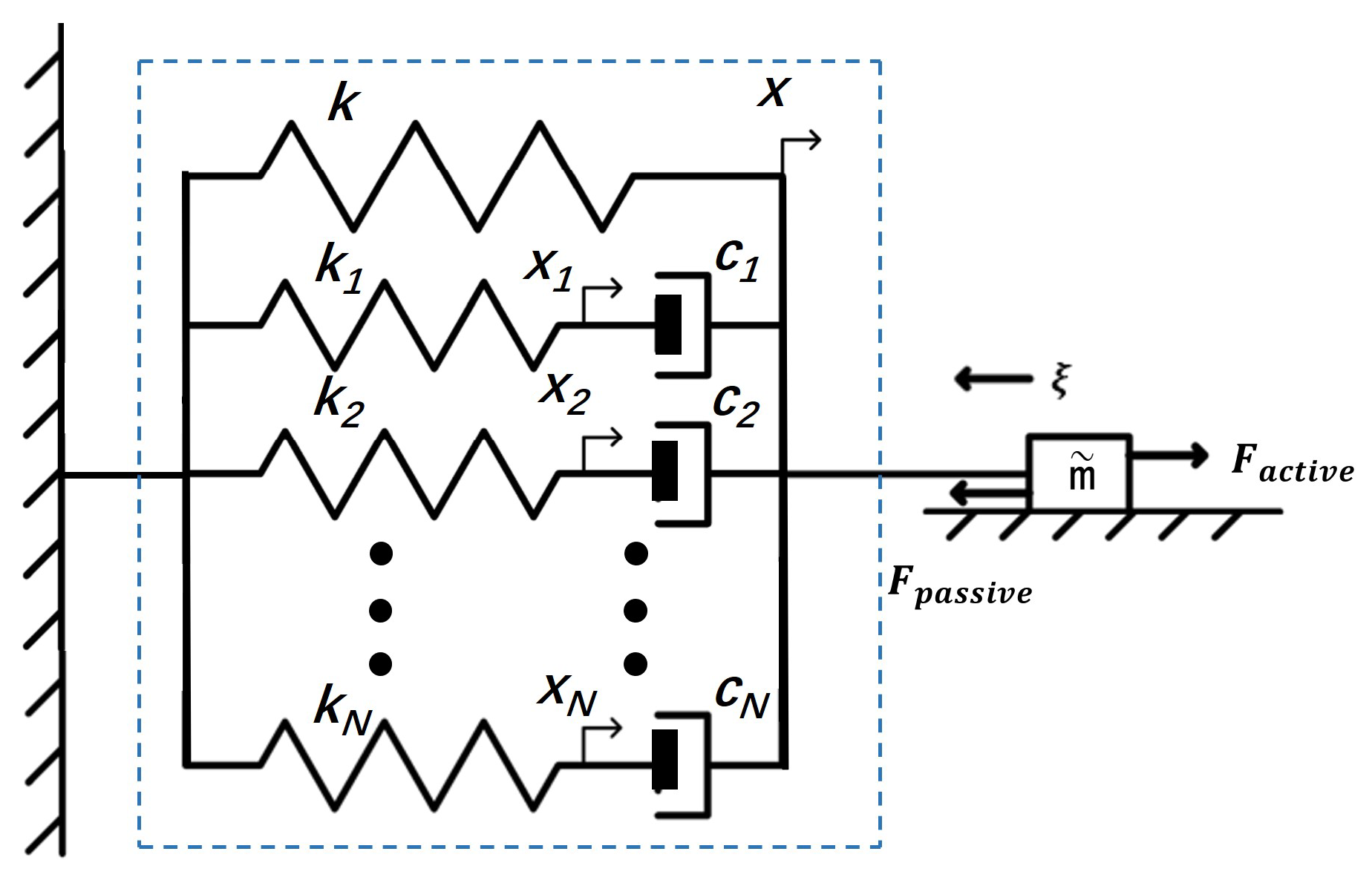
As shown in Figure 3, the decisive factors in the modeling process are the model parameters (i.e., linear spring stiffness k, spring stiffness $k_h$, viscous friction coefficient $c_h$, and system order N). These parameters are eventually determined through the system identification. $F_{active}$ refers to the active force produced by the system. In this paper, it is the contraction force generated by the PAM driven with high pressure. $F_{passive}$ refers to the passive damping force, including resistance force and other environmental stresses during the motion. Since the fixed environmental force can be directly included in the model parameters for simplification, only resistance force $\zeta$ would be concerned when considering the external effects. The model uncertainties are mainly due to the equivalent mass $\tilde{m}$ of the robotic system and the resistance force $\zeta$ during the motion. Hence, the dynamic equations for this system are given by

$$\tilde{m}\ddot{x}=-kx-\sum _{h=1}^N{k}_h{x}_h+F_{active}-\zeta sign\left(\dot{x}\right),$$

(8)

$$k_h{x}_h=c_h(\dot{x}-{\dot{x}}_h),h=1,2,\cdots ,N.$$

(9)

In this paper, the best fitting effect arises when $N=4$. Hence, the state-space model can be expressed as

$$\dot{X}=AX+Bu,$$

(10)

$$y=CX,$$

(11)

where

$$u=\frac{F_{active}+\tilde{f}}{\tilde{m}},F_{active}\ge 0,$$

(12)

$$\tilde{f}=-\zeta sign\left(\dot{x}\right),$$

(13)

$$X={\left[\begin{array}{cccccc}{x}_1& x_2& x_3& x_4& x& \dot{x}\end{array}\right]}^T,$$

(14)

$$A=\left[\begin{array}{cccccc}-k_1/c_1& 0& 0& 0& 0& 1\\ 0& -k_2/c_2& 0& 0& 0& 1\\ 0& 0& -k_3/c_3& 0& 0& 1\\ 0& 0& 0& -k_4/c_4& 0& 1\\ 0& 0& 0& 0& 0& 1\\ -k_1/\tilde{m}& -k_2/\tilde{m}& -k_3/\tilde{m}& -k_4/\tilde{m}& -k/\tilde{m}& 0\end{array}\right],$$

(15)

$$B={\left[\begin{array}{cccccc}0& 0& 0& 0& 0& 1\end{array}\right]}^T,$$

(16)

$$C=\left[\begin{array}{cccccc}0& 0& 0& 0& 1& 0\end{array}\right].$$

(17)

3.3. System Identification

According to (8) shown above, the system input is the resultant force $F_{active}$, and the output is the displacement x. However, in the actual operation process, it is difficult to provide the force signal directly. In the actuation with PAM, the actual input signal is pressure, and its output includes contraction force and deformation. Thus, the conversion relationship between force $F_{active}$ and pressure P should be established before system identification.

As can be seen in the actuation process of PAM, the contraction force increases as the input pressure increases, and it is directly associated with the end point’s movement under the unstrained case. In this paper, the end point’s movement equals to the system’s displacement, so it can be inferred that the contraction force is affected by both the pressure and the current displacement.

$$F_{active}=\omega (P,x).$$

(18)

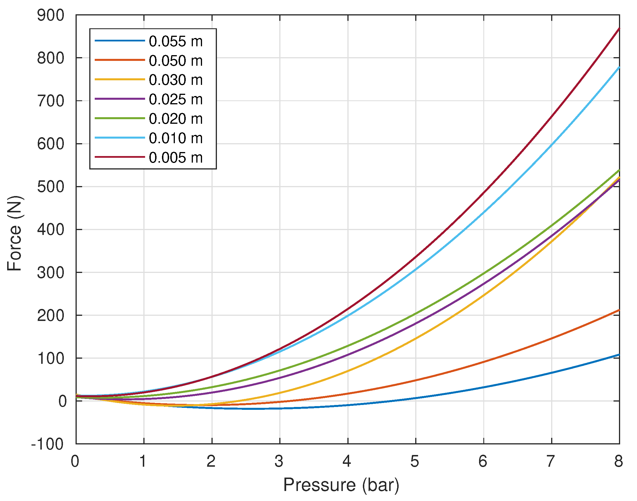
The force–pressure relationship of the PAM actuator is measured under isometric constraint, the experimental results are shown in Figure 4. Obviously, in the case of consistent displacement, the force–pressure curve has a strong linear characteristic, so (18) can be rewritten as

$$F_{active}=f_a\left(x\right)P+f_b\left(x\right).$$

(19)

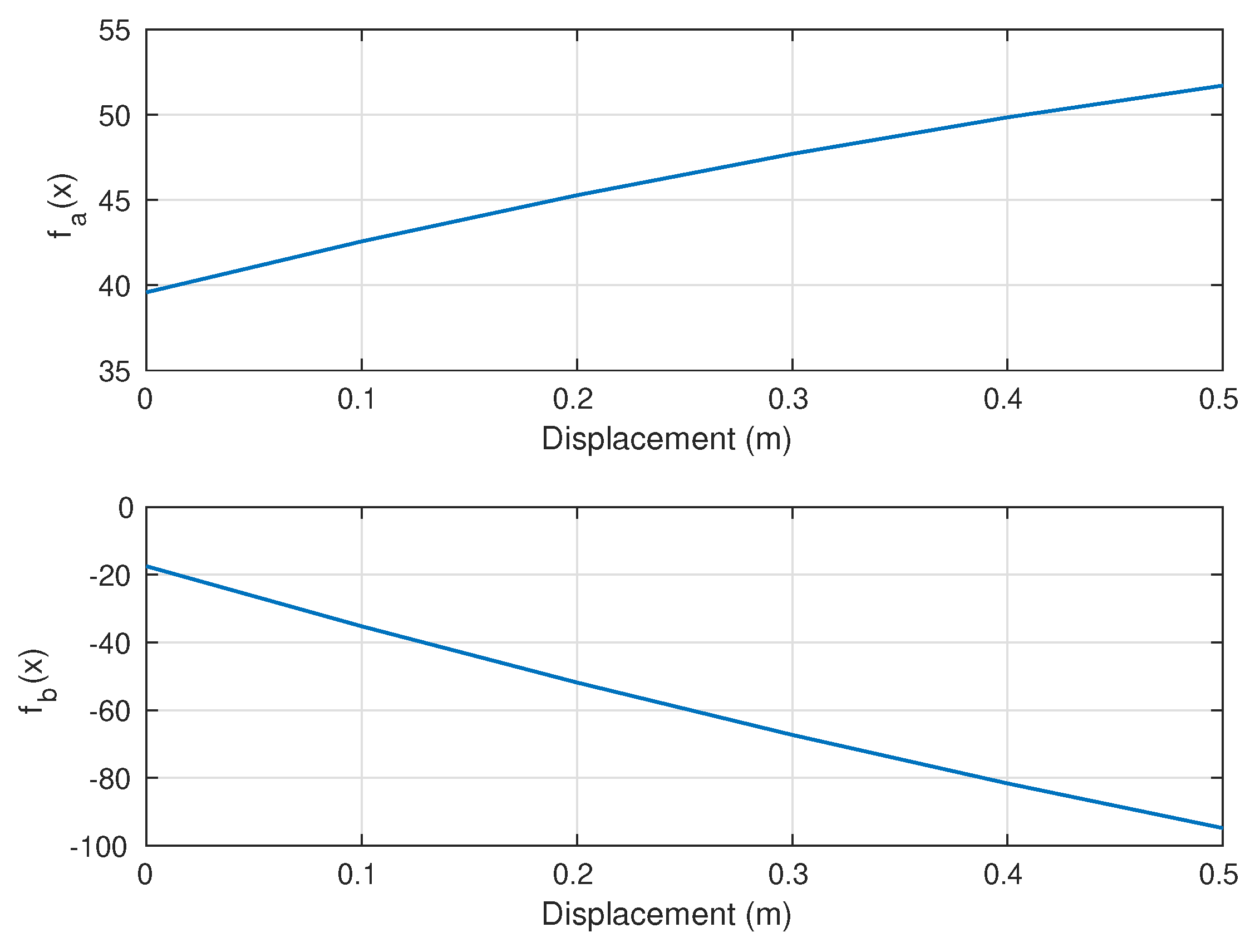
The specific expression of the force–pressure curve can be roughly determined through curve fitting method. The results are shown in Figure 5, whose coefficients of determination are $R^2=0.9878$.

Thus, the final expression of the force–pressure relationship is

$$\left\{\begin{array}{c}{F}_{active}=f_a\left(x\right)P+f_b\left(x\right)\hfill \\ f_a\left(x\right)=-14.046x^2+31.265x+39.584\hfill \\ f_b\left(x\right)=56.842x^2-183.05x-17.489\hfill \end{array}\right..$$

(20)

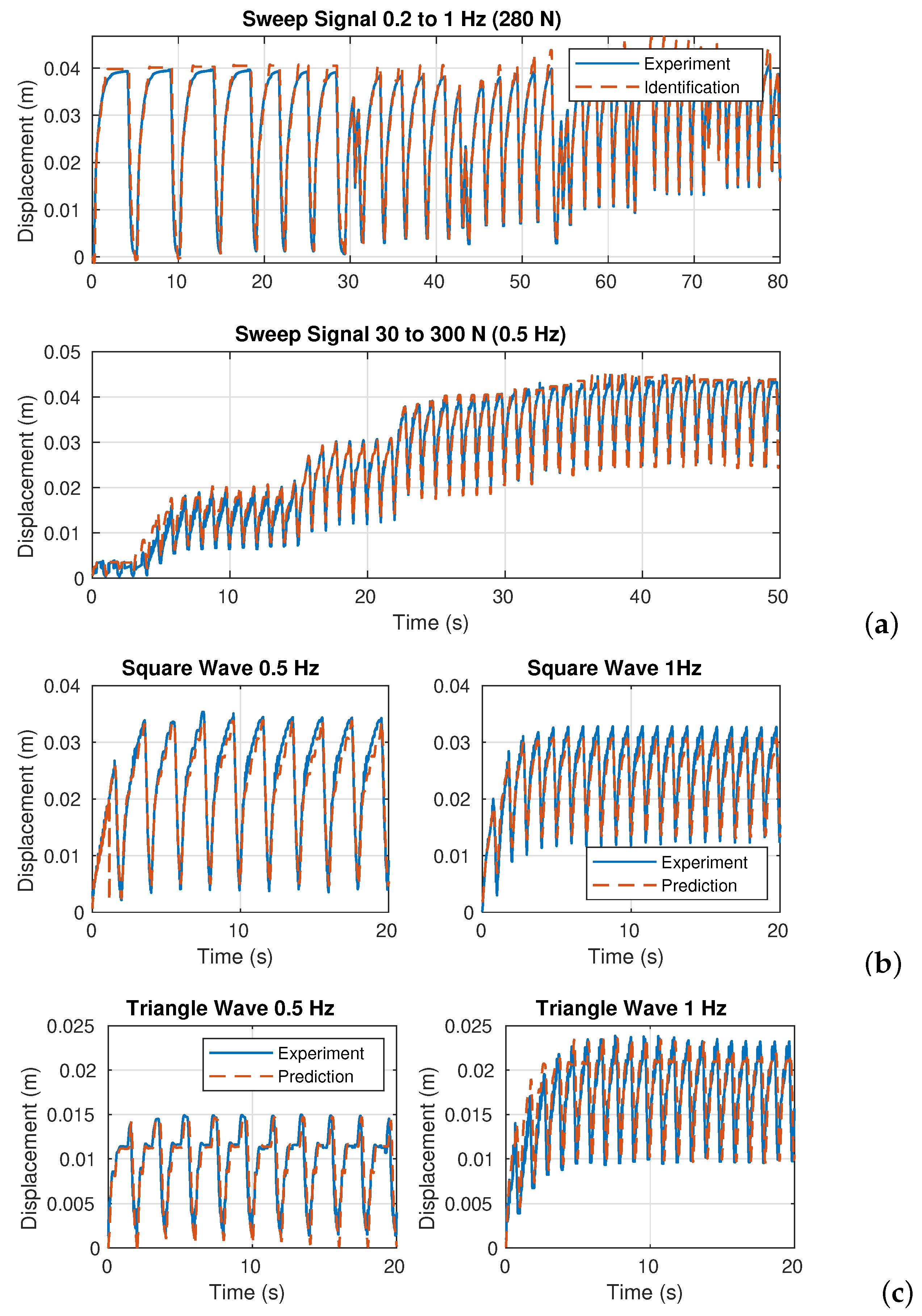
After the definition of the $F_{active}-P$ relationship, the system identification can be carried out. In this part, the data collected are mainly the input pressure and the output displacement. Here, the collected pressure data would be converted into actual contraction force data, which will be directly substituted into (8) for identification. In the experiment for system identification, a signal presented as a sinusoidal sweep force signal with the frequency of 0.2 to 1 Hz and the amplitude of 280 N is firstly applied to the PAM. To further improve the range of identification as well as the applicability, the PAM is also driven by another identification sinusoidal signal with the amplitude of 30 to 300 N and the frequency of 0.5 Hz. Following that, the System Identification Toolbox in MATLAB is used to estimate the parameters in (8) and (9). Figure 6a shows the identification result. Besides the identification, several regular signals (such as square wave and triangle wave) with a low frequency and a high frequency are also used to validate the identified model, the results of which are shown in Figure 6b,c.

Generally, the identified parameters are listed in

Table 1. The identified model parameters.

$\tilde{m}\left(kg\right)$		0.0893
$\zeta \left(N\right)$		$0.08\tilde{m}g$
$k(N·m^{-1})$		0.1768
$F_a[N·m^{-2}·ba{r}^{-1}N·m^{-1}·ba{r}^{-1}N·ba{r}^{-1}])$		$[-14.04631.26539.584]$
$F_b[N·m^{-2}·ba{r}^{-1}N·m^{-1}·ba{r}^{-1}N·ba{r}^{-1}])$		$[56.842-183.0517.489]$
$k_1(N·m^{-1})$	1.49	$c_1(N·m·s^{-1})$	0.06
$k_2(N·m^{-1})$	0.328	$c_2(N·m·s^{-1})$	0.09
$k_3(N·m^{-1})$	$7.144\times {10}^{-3}$	$c_3(N·m·s^{-1})$	0.447
$k_4(N·m^{-1})$	$2.5\times {10}^{-4}$	$c_4(N·m·s^{-1})$	0.857

. The identification accuracies of each curve are shown in

Table 2. Model accuracy of the identification and validation (MSE:mean squared error; MAPE: mean absolute percentage error; RMSE: root-mean-square error).

Curve Type		MSE	MAPE	RMSE	R-Squared
Identification	Sweep (0.2 to 1 Hz)	$5.7696\times {10}^{-6}$	0.1103	0.0024	0.9553
	Sweep (30 to 300 N)	$7.8242\times {10}^{-6}$	0.1102	0.0028	0.9565
Validation	Square (0.5 Hz)	$5.7253\times {10}^{-6}$	0.1183	0.0024	0.9312
	Square (1 Hz)	$6.2854\times {10}^{-6}$	0.1068	0.0025	0.8591
	Triangle (0.5 Hz)	$3.1551\times {10}^{-6}$	0.1163	0.0018	0.8701
	Triangle (1 Hz)	$5.1163\times {10}^{-6}$	0.1035	0.0023	0.8534

.

Since the displacement x has been taken as the actual output, the final output of the two PAMs can be expressed as

$$\left\{\begin{array}{c}{x}_1=L_1-L_{10}\hfill \\ x_2=L_2-L_{20}\hfill \end{array}\right..$$

(21)

As can be known from (7), the model of each PAM in the antagonistic pairs can be written as

$$\left\{\begin{array}{c}{\tilde{m}}_k{\ddot{x}}_k=-k_k{x}_k-\sum _{h=1}^4{k}_{kh}{x}_{kh}+F_{k,active}-{\zeta }_k\mathrm{sign}\left({\dot{x}}_k\right)\hfill \\ k_{kh}{x}_{kh}=c_{kh}({\dot{x}}_k-{\dot{x}}_{kh}),k=1,2\mathrm{and}h=1,2,\cdots ,N\hfill \end{array}\right.,$$

(22)

where $\mathrm{sign}\left({\dot{x}}_k\right)$ returns 1 or $-1$ depending on whether ${\dot{x}}_k$ is positive or negative, and

$$\left\{\begin{array}{c}{F}_1^{{}^{\prime }}=\frac{J\ddot{\theta }+F_2{d}_3-\chi (\theta ,\dot{\theta })}{l_F}\hfill \\ F_2^{{}^{\prime }}=\frac{-J\ddot{\theta }+F_1{l}_F+\chi (\theta ,\dot{\theta })}{d_3}\hfill \end{array}\right..$$

(23)

Thus,

$$\left\{\begin{array}{c}\begin{array}{ccc}\hfill {\ddot{x}}_k& =& (-\frac{k_k}{{\tilde{m}}_k}{x}_k-\frac{{\sum }_{h=1}^4{c}_{kh}}{{\tilde{m}}_k}{\dot{x}}_k)+\frac{1}{{\tilde{m}}_k}\sum _{h=1}^4{c}_{kh}{\dot{x}}_{k}h+\frac{f_{ka}\left(x_k\right)}{{\tilde{m}}_k}{P}_k+\frac{f_{kb}\left(x_i\right)+{\zeta }_k\mathrm{sign}\left({\dot{x}}_k\right)}{{\tilde{m}}_k}\hfill \\ \hfill & =& f_k(x_k,{\dot{x}}_k)+h_k\left({\dot{\tilde{x}}}_k\right)+f_{ka}\left(x_k\right)P_k+{\delta }_k\hfill \\ \hfill y_k& =& x_k\hfill \end{array}\hfill \end{array}\right.,$$

(24)

where ${\tilde{x}}_k={\left[x_{k1}{x}_{k2}{x}_{k3}{x}_{k4}\right]}^T$, and $P_k$ is the current inflation pressure of the k-th PAM.

Considering model uncertainties and disturbances, the following model is obtained

$$\begin{array}{c}\hfill \left\{\begin{array}{c}{\ddot{x}}_k=f_k(x_k,{\dot{x}}_k)+h_k\left({\dot{\tilde{x}}}_k\right)+f_{ka}\left(x_k\right)P_k+d_k\left(x_k\right)+{\delta }_k\hfill \\ =[\overline{f_k}(x_k,{\dot{x}}_k)+\delta f_k(x_k,\dot{x_k})]+[{\overline{h}}_k\left({\dot{\tilde{x}}}_k\right)+\delta h_k\left({\dot{\tilde{x}}}_k\right)]+[{\overline{f}}_{ka}\left(x_k\right)+\delta f_{ka}\left(x_k\right)]P_k\hfill \\ +d_k\left(x\right)+{\delta }_k\hfill \\ ={\overline{f}}_k(x_k,{\dot{x}}_k)+{\overline{h}}_k\left({\dot{\tilde{x}}}_k\right)+{\overline{f}}_{ka}\left(x_k\right)P_k+D_k(x_k,{\dot{x}}_k)\hfill \\ y_k=x_k\hfill \end{array}\right.\end{array}$$

(25)

where ${\overline{f}}_k(x_k,{\dot{x}}_k)$,${\overline{h}}_k\left({\dot{\tilde{x}}}_k\right)$ and ${\overline{f}}_{ka}\left(x_k\right)$ are the nominal models denoted by system identification, $\delta f_k(x_k,{\dot{x}}_k)$, $\delta h_k\left({\dot{\tilde{x}}}_k\right)$ and $\delta f_{ka}\left(x_k\right)$ are the model uncertainties, and $d_k\left(x_k\right)$ is the external disturbance. Lumping the model uncertainties, the external disturbances and the coupling effect together as $D_k(x_k,{\dot{x}}_k)\equiv \delta f_k(x_k,{\dot{x}}_k)+\delta h_k\left({\dot{\tilde{x}}}_k\right)+\delta f_{ka}\left(x_k\right)P_k+d_k\left(x_k\right)+{\delta }_k$, which is unknown but bounded. Specially, the bounded condition can be due to the mechanical constraints and the actuation limit.

Remarkably, the system can be considered as a bilinear system, which is an important subclass of nonlinear system [36]. Furthermore, the nonlinearity can come from the model uncertainties due to the system nonlinearity and the nonlinear components in the disturbance. Thus, each PAM in the antagonistic pairs can be treated as a nonlinear system with unknown but bounded uncertainties and disturbance.

4. Control Scheme

In this section, the control scheme for the developed robotic system is proposed and designed in detail.

4.1. Feedforward–Feedback Control Scheme

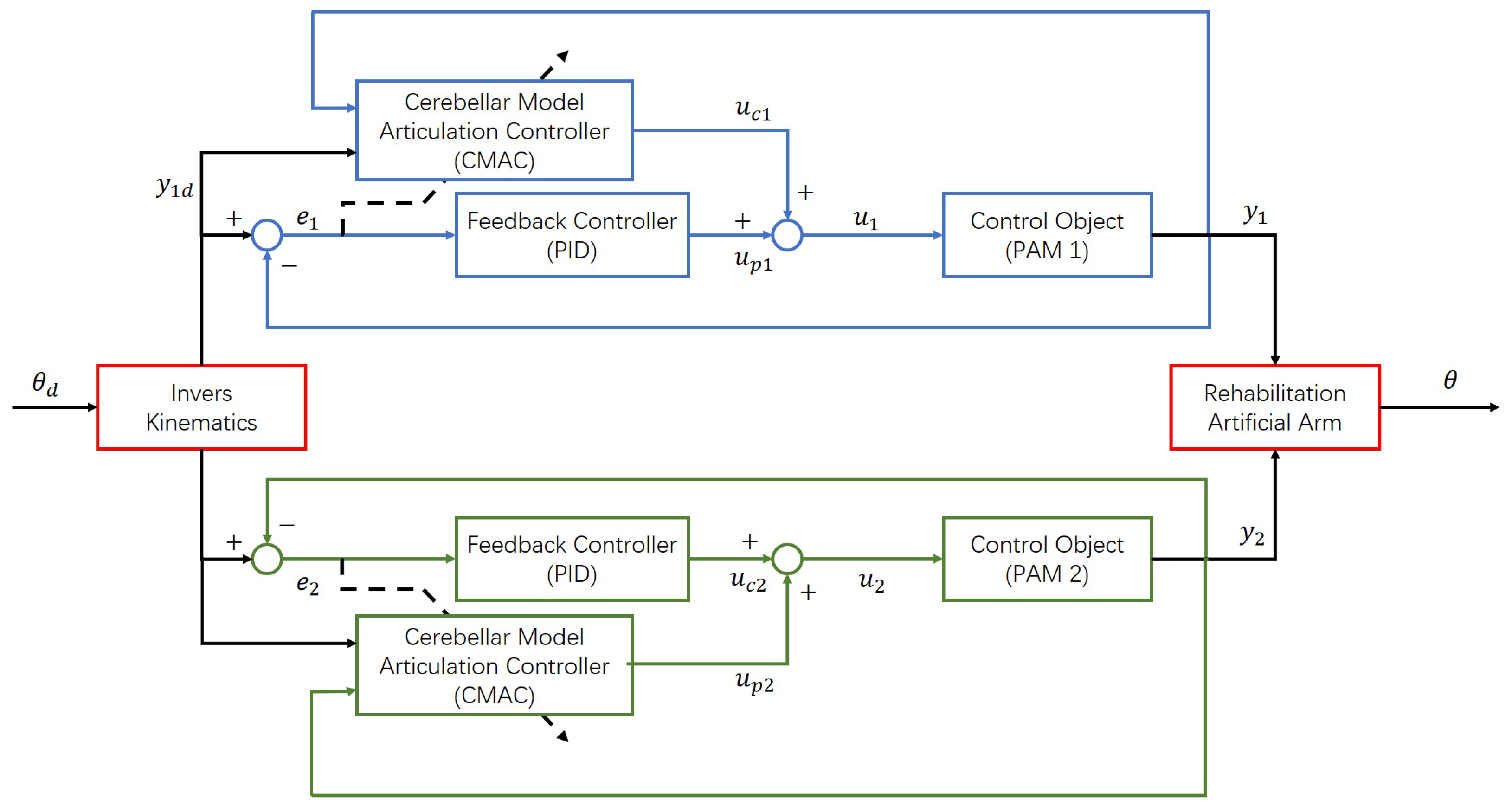
To ensure the control accuracy as well as a quick response, a feedforward–feedback control scheme is proposed in this paper, the block diagram of which is illustrated in Figure 7. Here, the feedback controller mainly refers to the error-based controller. It is worth noting that both PAMs are in the same control structure and therefore their control laws are significantly similar.

From (25), it shows that the ideal system input can be expressed as

$$\begin{array}{ccc}\hfill P_k& =& {\overline{u}}_k\hfill \\ \hfill & =& \frac{1}{{\overline{f}}_{ka}\left(x_k\right)}[{\ddot{x}}_{kd}-{\overline{f}}_k(x_k,{\dot{x}}_k)-{\overline{h}}_k\left({\dot{\tilde{x}}}_k\right)-D_k(x_k,{\dot{x}}_k)+k_p{e}_k+k_d{\dot{e}}_k]\hfill \\ \hfill & =& \frac{1}{{\overline{f}}_{ka}\left(x_k\right)}[{\ddot{x}}_{kd}-{\overline{f}}_{kd}(x_{kd},{\dot{x}}_{kd})-{\overline{h}}_k\left({\dot{\tilde{x}}}_{kd}\right)+\overline{C}(e_k,{\dot{e}}_k)-D_k(x_k,{\dot{x}}_k)]\hfill \\ \hfill & =& \frac{1}{{\overline{f}}_{ka}\left(x_k\right)}[{\ddot{x}}_{kd}-{\overline{f}}_{kd}(x_{kd},{\dot{x}}_{kd})-{\overline{h}}_k\left({\dot{\tilde{x}}}_{kd}\right)]+\frac{1}{{\overline{f}}_{ka}\left(x_k\right)}\overline{C}(e_k,{\dot{e}}_k)-\frac{1}{{\overline{f}}_{ka}\left(x_k\right)}{D}_k(x_k,{\dot{x}}_k)\hfill \\ \hfill & =& u_{feedforward}+u_{feedback}+\delta D,\hfill \end{array}$$

(26)

where $k_p$ and $k_d$ are two positive constants, $\overline{C}(e_k,{\dot{e}}_k)$ is the function of the motion error. As shown in the equation, the ideal controller can be regarded as a controller composed of feedforward control and feedback control essentially. $u_{feedforward}$ represents the feedforward control for desired motion, $u_{feedback}$ represents the feedback control for position error, and $\delta D$ denotes the compensation signal for uncertainties and disturbances.

Thus, a feedforward–feedback control scheme is suitable for the system developed in this paper. Moreover, a basic PID controller is adopted as the feedback controller due to its advantages of simple structure and easy implementation [37], the detailed design of which is shown below.

$$u_{pk}=K_{k,P}{e}_k+K_{k,I}\int e_{k}dt+K_{k,D}{\dot{e}}_k,$$

(27)

where $K_{k,P}$, $K_{k,I}$, $K_{k,D}$ are the proportional gain, the integral gain, the derivative gain, respectively, and $e_k$ is the motion error of the k-th actuator.

4.2. Cerebellar Model Articulation Controller

In this paper, the selection of the PAM actuator is due to its similarities to biological muscles, and the modified antagonistic structure is inspired from biological system. Therefore, developing a controller with bioinspiration can be a way to control this bio-inspired robot manipulator. In the spirit of this bio-inspired actuator, an artificial neural network controller based on the model of the mammalian cerebellum, namely, CMAC can be a good candidate [38].

Significantly, the functions of CMAC in the control scheme are mainly to approximate the feedforward controller mentioned above as well as to compensate for the disturbances because this neural network controller can offer good learning ability to approximate the system and even the nonlinear part. Meanwhile, the use of PID controller along with the CMAC can help the control system to stabilize the robot in the early phase which is good to improve the control system performance [39].

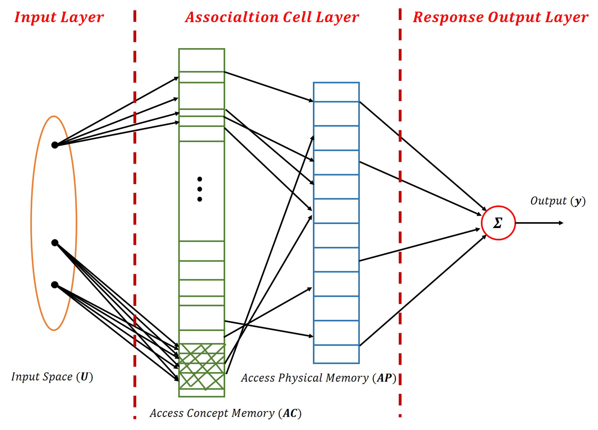
As observed from Figure 8, the CMAC is composed of three layers (input layer, association cell layer and response output layer) with two mappings (concept mapping and actual mapping). Then, the CAMC could be regarded as a pair of mappings given by

$$U\to AC\to AP\to y$$

(28)

where U denotes the input vectors, $AC$ and $AP$ represent Access Concept Memory and Access Physical Memory, respectively, and y denotes the output vector.

For the PAM, the control scheme with CMAC is illustrated in Figure 9. There are two inputs used in U: the displacement feedback information x and the desired motion reference $x_d$. Both signals are processed through the mappings and then the synaptic weights are located. Finally, the sum of the activated weights is sent as the control output to the system. Meanwhile, the weights are adjusted based on a rule with the objective of minimizing the motion error.

According to the cerebellar model, the detailed design of the CMAC is shown as follows.

(1) Input Quantization. To convert the continuous inputs into finite and discrete sets, the input vectors must be quantized. The uniform quantization interval is computed by

$$q_i=\frac{s_{i,max}-s_{i,min}}{r_i},i=1,2,$$

(29)

where $\mathbf{s}={\left[s_1{s}_2\right]}^T={\left[x{x}_d\right]}^T$ represents the input vector, $s_{i,max}=\max \left(s_i\right)$ and $s_{i,min}=\min \left(s_i\right)$ are the maximum and minimum of $s_i$, respectively, $r_i\in {\mathbb{N}}^{+}$ determines the quantization resolution, and $q_i$ is the number of the quantization interval.

In this step, the input space is divided into different regions. Each region is corresponding to a unique weight. Upon to the activation of the region, its corresponding weight will be activated.

(2) Association. To find out the regions needed to be activated corresponding to the current input vector, the Gaussian function is used as the basis function in this paper, which is expressed as

$${\phi }_{i{j}_i}\left(s_i\right)=\exp (-\frac{{(s_i-{\mu }_{i{j}_i})}^2}{{\sigma }_{i{j}_i}^2}),i=1,2\mathrm{and}{j}_i=1,2,\cdots ,n_i,$$

(30)

where ${\phi }_{i{j}_i}\left(s_i\right)$ represents the quantization distance of the i-th input $s_i$ to the $j_i$-th region, ${\mu }_{i{j}_i}$ represents the end points of the $j_i$-th region and ${\sigma }_{i{j}_i}$ represents the width of the $j_i$-th region. The number of the regions for the input $s_i$ could be defined as $n_i=q_i+1$. In this paper, the ${\mu }_{i{j}_i})$ and ${\sigma }_{i{j}_i}$ are set according to the quantization interval $q_i$, where ${\sigma }_{i{j}_i}$ is set equally in each region, which means ${\sigma }_{i{j}_i}={\sigma }_i$. Evidently, a larger $n_i$ can cause a higher resolution, but a more complex computation.

The basis function used in this paper is defined as

$$G_j\left(\mathbf{s}\right)=\prod _{i=1}^2{\phi }_{i{j}_i}\left(s_i\right)=\exp (\sum _{i=1}^2-\frac{{(s_i-{\mu }_{i{j}_i})}^2}{{\sigma }_{i{j}_i}^2}),j=1,2,\cdots ,n_r\mathrm{and}{j}_i=1,2,\cdots ,n_i,$$

(31)

where $n_r=n_1\times n_2$ denotes the number of the respective fields. In another way, the mapping vector can be expressed by the form of

$$\varphi \left(s\right)={[G_1{G}_2\cdots G_{n_r}]}^T.$$

(32)

(3) Output. The output of the CMAC is the sum of the activated weights in the weight memory w:

$$u_c=\prod _{j=1}^{n_r}{w}_j{G}_j={\tilde{w}}^T\varphi ,$$

(33)

where $u_c=u_{CMAC}$ is the output of controller to the system, $\tilde{w}={[w_1{w}_2\cdots w_{n_r}]}^T\in {\mathbb{R}}^n$ denotes the estimated weight vector.

(4) Weight Update. To adjust the weights in each cycle, the $\delta$ learning rule [40] is employed, then the weight adjustment index is defined by

$$Q\left(\tilde{w}\right)=\frac{1}{2}{\epsilon }^2,$$

(34)

where $\epsilon =\ddot{e}+k_d\dot{e}+k_{p}e$ is the filter error and $e=x_d-x$ is the motion error. The objective of CMAC is to minimize the adjustment evaluation function $Q\left(\tilde{w}\right)$.

By applying the gradient descent algorithm, the learning law is given by

$${\tilde{w}}^{p+1}={\tilde{w}}^p-\eta \frac{\partial Q}{\partial \tilde{w}},$$

(35)

where p denotes the p-th iteration and $\eta$ is the learning rate.

Substitute $u_c$ into (25), the error model of the system can be expressed as

$$\dot{E}=\left[\begin{array}{cc}0& 1\\ -k_p& -k_d\end{array}\right]E+\left[\begin{array}{c}0\\ {\overline{f}}_{ia}\left(x\right)\end{array}\right]e_u,$$

(36)

where $e_u=\overline{u}-u_c$ is the approximation error between the desired control output $\overline{u}$ and the actual CMAC control output $u_c$, $E={\left[e\dot{e}\right]}^T$ represents the error state. Thus, we have

$${\overline{f}}_{ia}\left(x\right)(\overline{u}-u_c)={\overline{f}}_{ia}\left(x\right)(\overline{u}-\prod _{j=1}^{n_r}{w}_j{G}_j)=\ddot{e}+k_d\dot{e}+k_{p}e=\epsilon .$$

(37)

Hence,

$$\frac{\partial Q}{\partial \tilde{w}}=\frac{\partial Q}{\partial \epsilon }\frac{\partial \epsilon }{\partial \tilde{w}}=-\epsilon {\overline{f}}_{ia}\left(x\right)\varphi .$$

(38)

Then, the learning law is given by

$${\tilde{w}}^{p+1}={\tilde{w}}^p+\eta \epsilon {\overline{f}}_{ia}\left(x\right)\varphi .$$

(39)

In the designed CMAC, because the learning law is related to the filter error, which is determined by the motion error, an adaptive control is formed.

As the two actuators have a similar control law, the CMAC controller could be given by

$$u_{ck}={\tilde{w}}_k^T{\varphi }_k,$$

(40)

where $k=1,2$ represents the first actuator PAM1 and the second actuator PAM2, respectively.

Hence, the whole controller, combining the adaptive CMAC and the PID controller, is shown as follows.

$$\begin{array}{ccc}\hfill u_k& =& u_{ck}+u_{pk}\hfill \\ \hfill & =& {\tilde{w}}_k^T{\varphi }_k+K_{k,P}{e}_k+K_{k,I}\int e_{k}dt+K_{k,D}{\dot{e}}_k.\hfill \end{array}$$

(41)

5. Simulation and Experimental Results

In this section, both simulations and experiments are carried out to evaluate the control performance of the proposed feedforward–feedback control scheme.

5.1. Simulation

The parameters used in the simulation are given in Table 1. According to the demand in medical rehabilitation of stroke patients, a proper trajectory is the periodic repeatable motion between the target position and the initial relaxation position ($\theta =0$).

For the purpose of verifying the control performance of the proposed system, the following three simulations are conducted to evaluate the control performance.

(1) Single PAM control simulation.

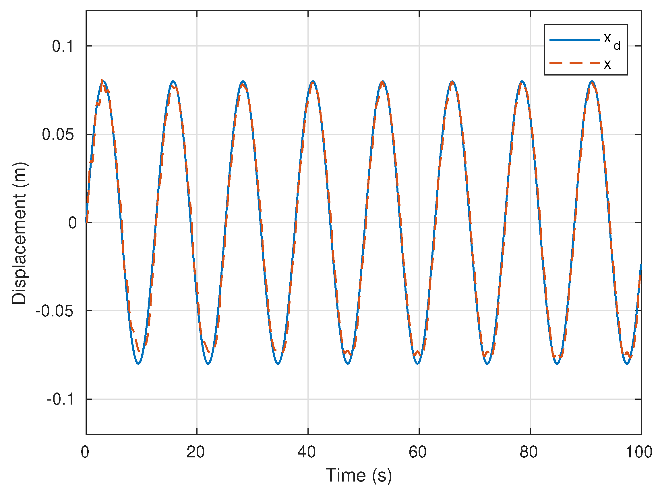
As mentioned in Section 4, the feedforward–feedback control scheme is composed of CMAC and PID controllers. A sinusoidal trajectory with an amplitude of $0.08$ m is used in the simulation.

For the comparison purpose, the control schemes and controllers are applied to the system: (i) PID-only, (ii) CMAC-only, and (iii) feedforward–feedback.

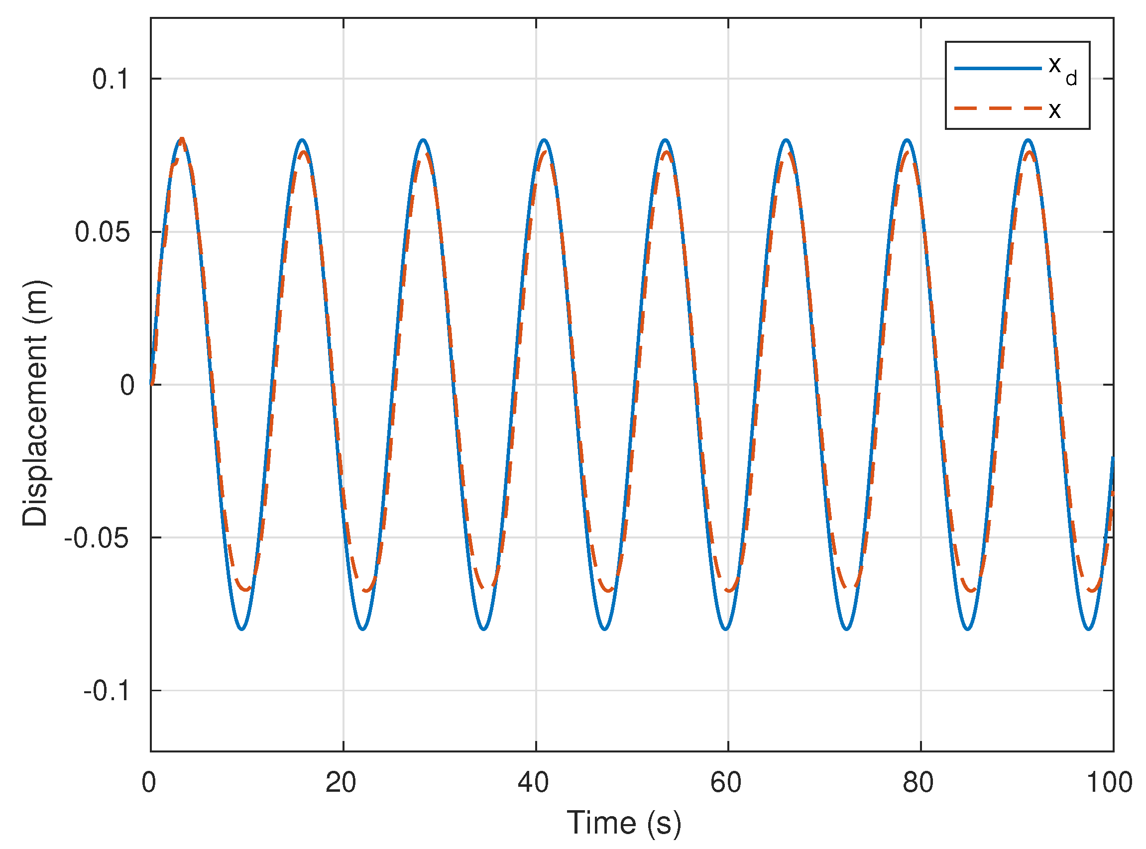
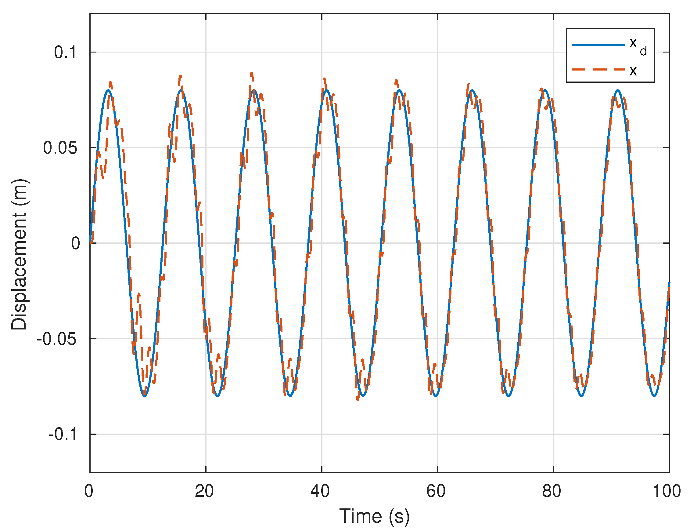
Figure 10, Figure 11 and Figure 12 shows the control results with the PID-only, CMAC-only, and feedforward–feedback control schemes, respectively.

As shown in Figure 12, the PID-only control scheme can achieve a good tracking performance, but there is a certain response lag in each cycle. By comparing the PID-only control scheme with the CMAC-only control scheme, the CMAC-only control scheme can also help the system to track the desired trajectory, but the trajectory tracking error is smaller while using the PID-only control scheme.

After applying the feedforward–feedback control scheme, combining the CMAC and PID controller, the tracking performance is shown in Figure 12, the improvement of the response is apparent. From the results, both response speed and accuracy are satisfactory. This is because the system nonlinearity can be well handled by the CMAC and the feedforwad control can help to shorten the response time. This shows the advantages of applying the CMAC in the proposed control scheme.

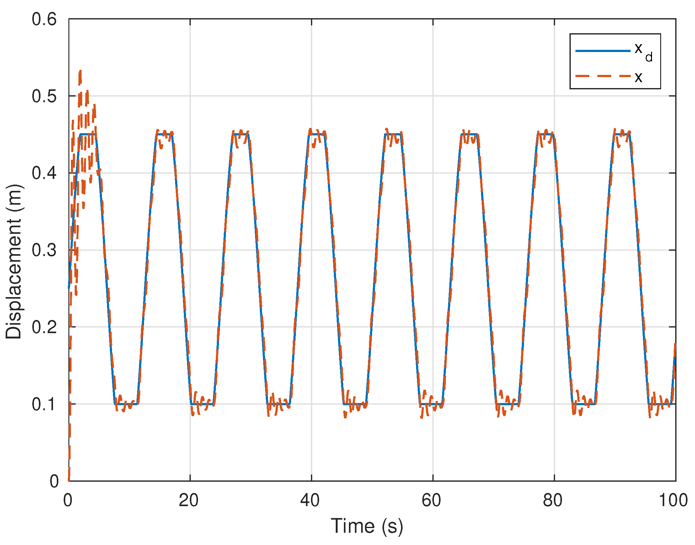
Considering the practical application (repetitive rehabilitation), the saturated sinusoidal trajectory is used as the desired motion trajectory. As shown in Figure 13, the displacement (length) of PAM switches periodically between $0.01$ m and $0.045$ m, mimicking the deformation process of biological muscle in a repetition motion. The result shown in Figure 13 is consistent with the previous simulation results. It can achieve good performance in terms of response speed and accuracy in each cycle, but some errors still exist at the peaks of the trajectories.

(2) PAMs in antagonistic pairs control simulation.

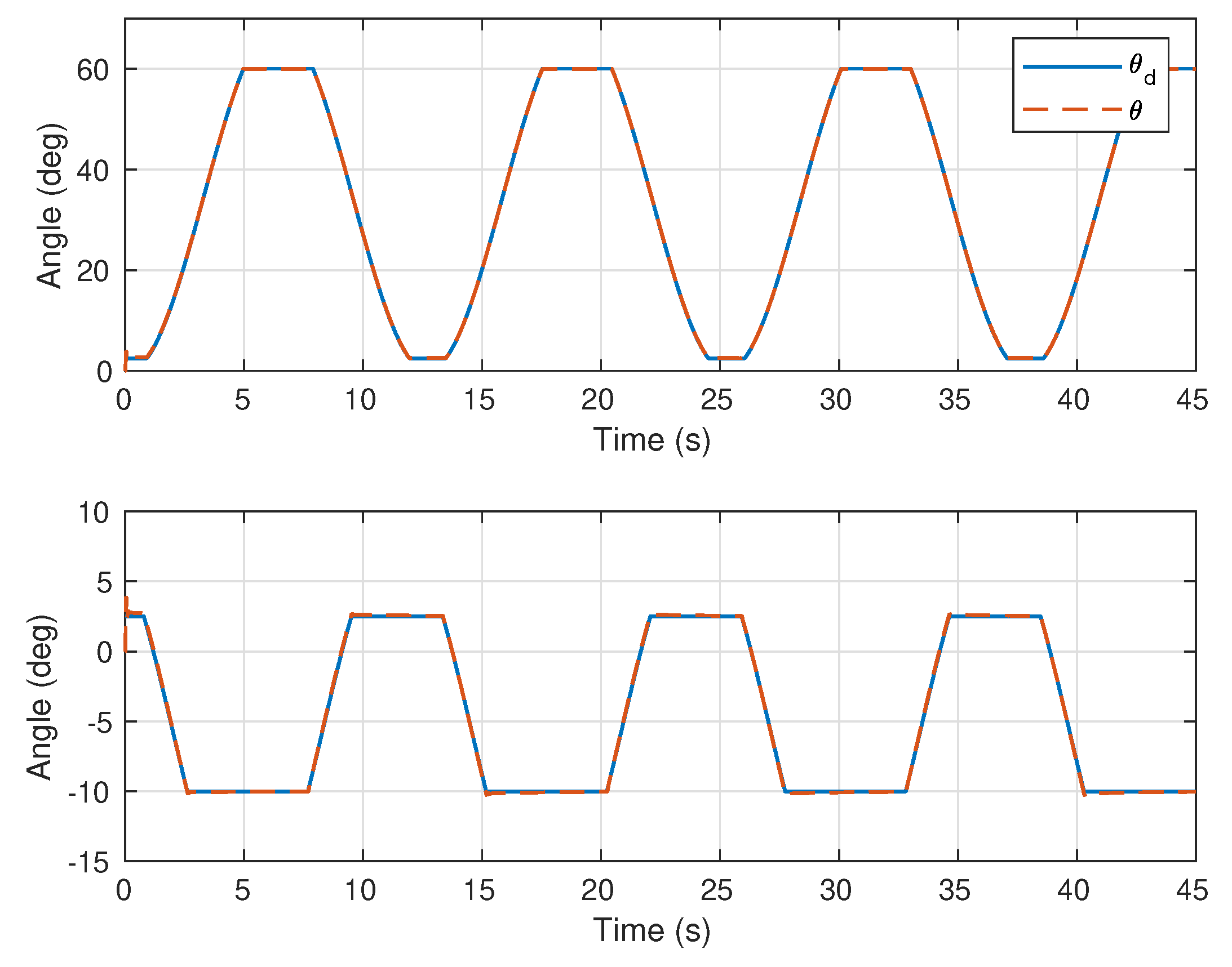
After the simulation of a single PAM, it is necessary to evaluate the control performance of the manipulator with antagonistic pairs. Similarly, with the consideration of practical application, the desired trajectories are set as the saturated sinusoidal trajectory. Furthermore, with the concern of the special case, both sides of rotation should be tested. Here, the positive rotation ranges from $2.5^{\circ }$ to ${60}^{\circ }$, and the negative rotation from $2.5^{\circ }$ to $-{10}^{\circ }$ (the manipulator that hangs naturally has a slight angle instead of $0^{\circ }$) are tested.

Figure 14 shows the simulation results on the trajectory tracking with the manipulator using the proposed control scheme. As can be seen, both desired trajectories in the bidirectional rotation can be well tracked. By comparing these results to the control of the single PAM, it can be found out that the response speed and accuracy can be improved with the assistance of the antagonistic pairs.

(3) PAMs in antagonistic pairs control simulation with uncertainty and disturbance.

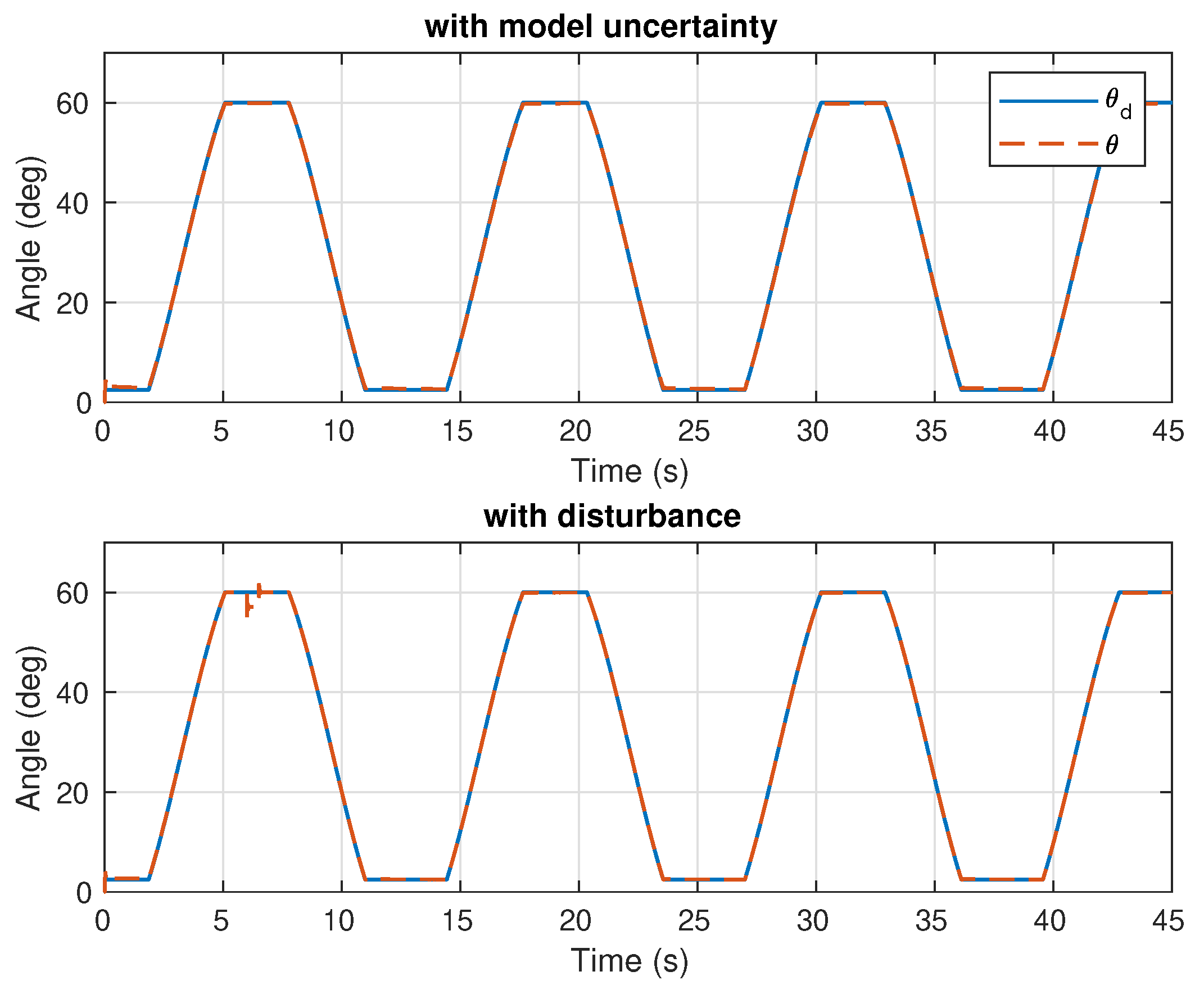
To evaluate the robustness of the proposed system, simulation while the uncertainty and disturbance are added to the system is carried out, respectively. Two situations are tested in this simulation, the first one is to increase the equivalent mass of the whole system to be two times of the identified equivalent mass, which represents the model uncertainty, and the second one is to introduce an input disturbance into the system after about five seconds.

Figure 15 shows the control system tracking performance under these two situations. As can be observed from the figure, the proposed control scheme is still able to help the system to track the desired trajectories well no matter there is an uncertainty or a disturbance exist in the system. Therefore, it can be concluded that the proposed control scheme can achieve guaranteed robustness.

In all, the simulation results indicate that the proposed feedforward–feedback control scheme performs well on the motion trajectory tracking of the rehabilitation pneumatic robotic device.

5.2. Experiments

To further validate the effectiveness and feasibility of the proposed control scheme, real-time experiments of motion trajectory tracking have been conducted in a practical experimental system setup shown in Figure 16. In this setup, two PAMs (FESTO, DMSP-10-200N-RM-CM) are used in antagonistic pairs to construct the robot manipulator. Two solenoid switching valves (MHE2-MS1H-3/2G-QS4-K) are used to control inflation/deflation of the PAMs and four solenoid valves (MHJ10-S-2.5-QS-4-MF) are used to adjust the airflow to the PAMs. Furthermore, two pressure sensors (SPTE-P10R-Q4-B-2.5K) are used to measure the pressure inside the two PAMs, respectively. Moreover, an OptiTrack motion capture system (with five cameras) is used to measure the displacements of the PMAs and the rotation angle of the manipulator. Lastly, a computer is used to receive the sensing information, implement the proposed control scheme, send out the control input signals to the robot manipulator.

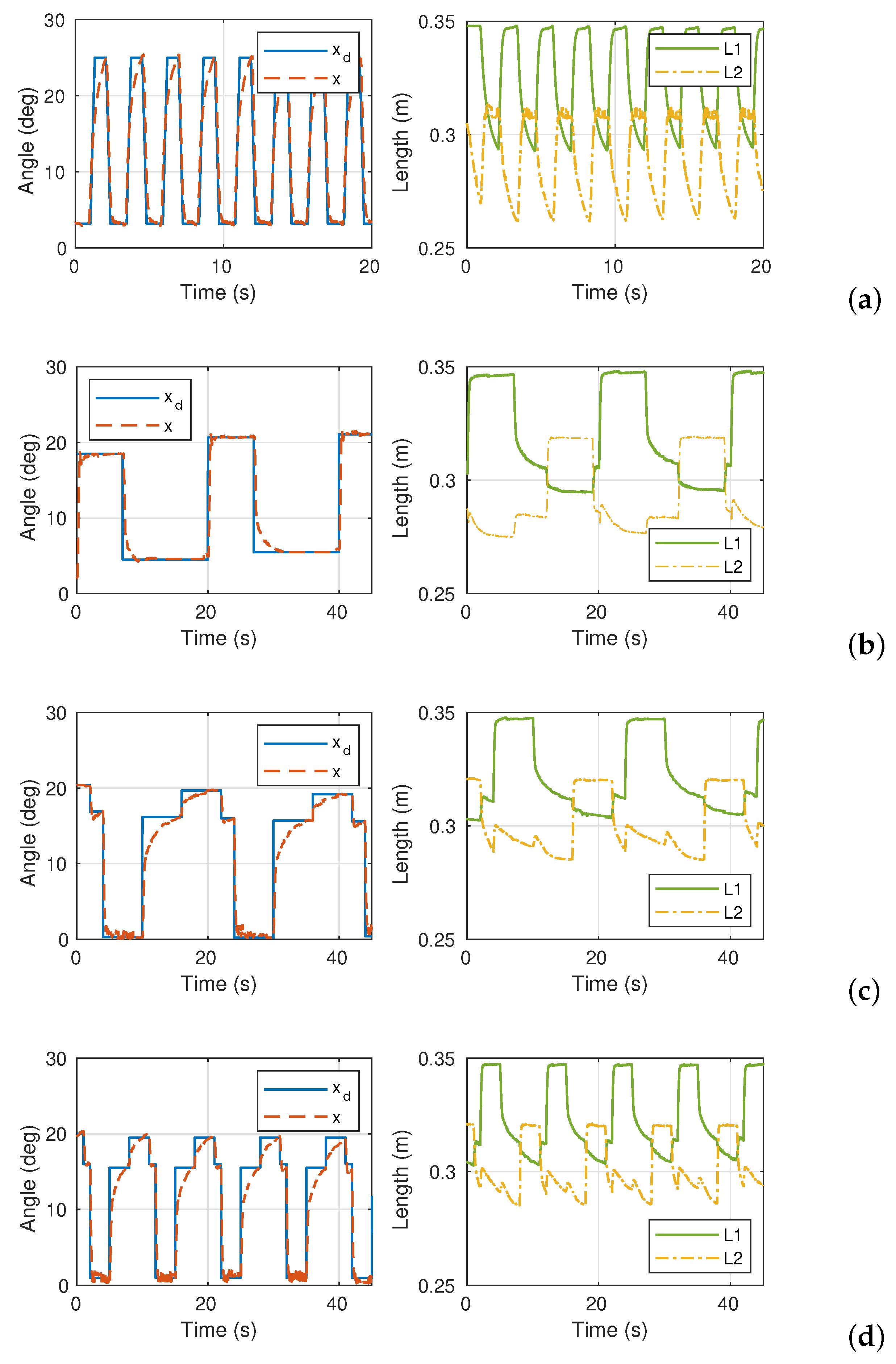
Considering that keeping the arm in the elbow flexion state for a period of time is more effective in the arm rehabilitation training, the sinusoidal wave is replaced by four more appropriate trajectories in the real-time experiment. Four different experiments are carried out to explore the effectiveness of the proposed rehabilitation pneumatic robotic device with antagonistic pairs. The results are evaluated by the displacement accuracy of the PAMs and the rotation angle error of the manipulator.

(1) High-frequency trapezoidal trajectory.

In this paper, the antagonistic pairs are prepared for the large displacement and/or high-speed operations, thus this property should be tested. As shown in Figure 17a, a trapezoidal wave with a high frequency of 2.6 Hz is set as the desired trajectory, ensuring that the manipulator rotates from $3.2^{\circ }$ to ${25}^{\circ }$ periodically.

From the results, the actual motion tracks well with the desired trajectory in spite of little lag. Due to the high frequency, the response is not timely in the rising edge stage, but it still can achieve the target position finally at the steady state.

(2) Stepped high amplitude square trajectory.

This experiment is designed to verify the feasibility in various large displacement situation. In this part, a square signal with changing amplitude of around ${20}^{\circ }$ is applied. As shown in Figure 17b, the manipulator performs well with the low frequency and large amplitude desired trajectories, but it is still a bit slow at the rise time. Considering that the overshoot and the steady state error are more important for a rehabilitation device, the tracking performance on this square trajectory is satisfactory for the rehabilitation application. Besides that, the gradually changing amplitude can assist the patients in increasing their motion range gradually rather than abruptly.

(3) Low-frequency convex trajectory:

To achieve a better auxiliary effect, it is necessary to design a trajectory according to the biological behavior and rehabilitation goals. The purpose of the previous two experiments is to verify the effectiveness of the control scheme and the manipulator, and its evaluation is determined by the response speed and accuracy. However, it is not sufficient for practical medical applications. For example, the speed of motion should be limited to ensure the smoothness of the trajectory and avoid the cause of secondary injury during the recovery process. The rehabilitation course should also be gradual, which means that each course of treatment should be improved on the basis of the last course of treatment, it cannot be abrupt.

Referring to the above considerations on the practical application, a convex trajectory was designed and the rotation rate was limited (a speed controller as the main circuit is added, forming a kind of cascade control). As shown in Figure 17c, the system has a fast response and is able to reach the desired position eventually. In the tracking process, the actual angle of the manipulator increases gently, which puts little load on the arm and provides a period of adaptive phase. It should be pointed out that the rehabilitation device is essentially a passive device, and thus the human–robot interaction should be emphasized when assisting body movements. Otherwise, the therapeutic effect can hardly be improved, and it might cause even worse malignant effects.

According to the results of this experiment, it can be determined that the proposed system could meet the design expectation for actual application with the low-frequency convex trajectory. To be specific, the manipulator will enlarge its motion range. In this experiment, assuming that the patients have already adapted to the motion range from ${0.2}^{\circ }$ to ${16}^{\circ }$, then extending the upper range of the motion to ${19}^{\circ }$, and thus the motion range from $0.2^{\circ }$ to ${19}^{\circ }$, is set as the new goal of rehabilitation. Considering the exercise load and rehabilitation efficiency, the motion phase is divided into two steps. In the first step, the angle rotates from $0.2^{\circ }$ to ${16}^{\circ }$. Then in the second step, the angle rotates from ${16}^{\circ }$ to ${19}^{\circ }$. In this way, the patients only need to concentrate on the rehabilitation training with the motion range from ${16}^{\circ }$ to ${19}^{\circ }$. After adapting to the new extended range, the integrated square-like trajectory will be applied for a new training. Repeat the above process, the patients would increase their exercisable motion range step by step.

(4) High-frequency convex trajectory.

Based on the third experiment, a repeated experiment is carried out with a high-frequency convex trajectory in order to further demonstrate the feasibility of rehabilitation. In the third experiment, the reason to choose convex trajectory has been explained, and the design of the rehabilitation project has also been introduced. However, a crucial transition phase should be added in the above rehabilitation process, i.e., the high-frequency motion stage. Apparently, the low-frequency movements occupy a major part in the rehabilitation to allow the patients to adapt to various motions. However, the accomplishment of high-frequency movements can help to reflect the recovery effect. Thus, a gradual training process from low frequency to high frequency is indispensable for any motion in rehabilitation.

Hence, in this experiment, another convex trajectory with a higher frequency but the same amplitude is applied, the results of which are shown in Figure 17d. From the figure, the actual motion can achieve the desired target at the end of the response. There is a difference between the desired trajectory and the actual trajectory due to the added design with the motion speed limitation. In spite of this, the system performs well on the motion trajectory tracking.

In summary, although the rise time is a bit slow, the steady state is very accurate where the steady state errors under the high-frequency trajectory and the low-frequency trajectory are within 0.8${}^{\circ }$ and 0.5${}^{\circ }$, respectively. According to the results and analysis shown above, it can be revealed that the proposed control scheme is effective for the motion trajectory tracking with the developed manipulator, which helps the system achieve good tracking performance for the medical application.

6. Conclusions

In this paper, the control issues of a rehabilitation robotic device driven by soft PAMs for stroke patients has been investigated. The main challenge of the control issues lies in the difficulty of dealing with the nonlinearity and the passive recovery characteristic. To overcome the challenges, an antagonistic coupling structure and a feedforward–feedback control scheme are proposed. Moreover, for medical applications, a rehabilitation robotic device driven by two PAMs in antagonistic pairs is designed.

To verify the feasibility of the proposed medical rehabilitation robotic device, both theoretical analysis as well as simulations and experiments are conducted. The results show that the designed robotic system can achieve a good control performance with the proposed control scheme. Furthermore, the applicability with a more complex and flexible medical rehabilitation robotic device will be studied in future work.

References

1. World Health Organization. Neurological Disorders: Public Health Challenges; World Health Organization: Geneva, Switzerland, 2006. [Google Scholar]
2. Johnson, C.O.; Nguyen, M.; Roth, G.A.; Nichols, E.; Alam, T.; Abate, D.; Abd-Allah, F.; Abdelalim, A.; Abraha, H.N.; Abu-Rmeileh, N.M.; et al. Global, regional, and national burden of stroke, 1990–2016: A systematic analysis for the Global Burden of Disease Study 2016. Lancet Neurol. 2019, 18, 439–458. [Google Scholar] [CrossRef] [Green Version]
3. Nakayama, H.; Jrgensen, H.S.; Raaschou, H.O.; Olsen, T.S. Recovery of upper extremity function in stroke patients: The Copenhagen Stroke Study. Arch. Phys. Med. Rehabil. 1994, 75, 394–398. [Google Scholar] [CrossRef]
4. Van Peppen, R.P.; Kwakkel, G.; Wood-Dauphinee, S.; Hendriks, H.J.; Van der Wees, P.J.; Dekker, J. The impact of physical therapy on functional outcomes after stroke: What’s the evidence? Clin. Rehabil. 2004, 18, 833–862. [Google Scholar] [CrossRef] [PubMed]
5. Lu, R.; Li, Z.; Su, C.Y.; Xue, A. Development and Learning Control of a Human Limb With a Rehabilitation Exoskeleton. Ind. Electron. IEEE Trans. 2014, 61, 3776–3785. [Google Scholar] [CrossRef]
6. Andrikopoulos, G.; Nikolakopoulos, G.; Manesis, S. A survey on applications of Pneumatic Artificial Muscles. In Proceedings of the 2011 19th Mediterranean Conference on Control and Automation, MED 2011, Corfu, Greece, 20–23 June 2011; pp. 1439–1446. [Google Scholar]
7. Ranzani, T.; Cianchetti, M.; Gerboni, G.; Falco, I.D.; Menciassi, A. A soft modular manipulator for minimally invasive surgery: Design and characterization of a single module. IEEE Trans. Robot. 2016, 32, 187–200. [Google Scholar] [CrossRef]
8. Deng, Z.; Stommel, M.; Xu, W. Mechatronics design, modeling, and characterization of a soft robotic table for object manipulation on surface. IEEE/ASME Trans. Mechatron. 2018, 23, 2715–2725. [Google Scholar] [CrossRef]
9. Wang, W.; Ahn, S.H. Shape memory alloy-based soft gripper with variable stiffness for compliant and effective grasping. Soft Robot. 2017, 4, 379–389. [Google Scholar] [CrossRef]
10. Motzki, P.; Khelfa, F.; Zimmer, L.; Schmidt, M.; Seelecke, S. Design and Validation of a reconfigurable Robotic End-Effector Based on Shape Memory Alloys. IEEE/ASME Trans. Mechatron. 2019, 24, 293–303. [Google Scholar] [CrossRef]
11. Cao, J.; Liang, W.; Ren, Q.; Gupta, U.; Chen, F.; Zhu, J. Modelling and control of a novel soft crawling robot based on a dielectric elastomer actuator. In Proceedings of the 2018 IEEE International Conference on Robotics and Automation (ICRA), Brisbane, QLD, Australia, 21–25 May 2018; pp. 4188–4193. [Google Scholar]
12. Gu, G.Y.; Gupta, U.; Zhu, J.; Zhu, L.M.; Zhu, X. Modeling of viscoelastic electromechanical behavior in a soft dielectric elastomer actuator. IEEE Trans. Robot. 2017, 33, 1263–1271. [Google Scholar] [CrossRef]
13. Onal, C.D.; Rus, D. Autonomous undulatory serpentine locomotion utilizing body dynamics of a fluidic soft robot. Bioinspir. Biomim. 2013, 8, 026003. [Google Scholar] [CrossRef]
14. Fras, J.; Noh, Y.; Macias, M.; Wurdemann, H.; Althoefer, K. Bio-inspired octopus robot based on novel soft fluidic actuator. In Proceedings of the 2018 IEEE International Conference on Robotics and Automation (ICRA), Brisbane, QLD, Australia, 21–25 May 2018; pp. 1583–1588. [Google Scholar]
15. Gong, Z.; Cheng, J.; Chen, X.; Sun, W.; Fang, X.; Hu, K.; Xie, Z.; Wang, T.; Wen, L. A bio-inspired soft robotic arm: Kinematic modeling and hydrodynamic experiments. J. Bionic Eng. 2018, 15, 204–219. [Google Scholar] [CrossRef]
16. Tsagarakis, N.G.; Caldwell, D.G. Development and Control of a ’Soft-Actuated’ Exoskeleton for Use in Physiotherapy and Training. Auton. Robot. 2003, 15, 21–33. [Google Scholar] [CrossRef]
17. Daerden, F.; Lefeber, D. Pneumatic artificial muscles: Actuators for robotics and automation. Eur. J. Mech. Environ. Eng. 2002, 47, 10–21. [Google Scholar]
18. Sugar, T.G.; He, J.; Koeneman, E.J.; Koeneman, J.B.; Herman, R.; Huang, H.; Schultz, R.S.; Herring, D.E.; Wanberg, J.; Balasubramanian, S.; et al. Design and control of RUPERT: A device for robotic upper extremity repetitive therapy. IEEE Trans. Neural Syst. Rehabil. Eng. 2007, 15, 336–346. [Google Scholar] [CrossRef] [PubMed]
19. Balasubramanian, S.; Wei, R.; Perez, M.; Shepard, B.; Koeneman, E.; Koeneman, J.; He, J. RUPERT: An exoskeleton robot for assisting rehabilitation of arm functions. In Proceedings of the 2008 Virtual Rehabilitation, Vancouver, BC, Canada, 25–27 August 2008; 2008; pp. 163–167. [Google Scholar]
20. Huang, J.; Tu, X.; He, J. Design and evaluation of the RUPERT wearable upper extremity exoskeleton robot for clinical and in-home therapies. IEEE Trans. Syst. Man Cybern. Syst. 2016, 46, 926–935. [Google Scholar] [CrossRef]
21. Nef, T.; Mihelj, M.; Colombo, G.; Riener, R. ARMin—Robot for rehabilitation of the upper extremities. In Proceedings of the 2006 IEEE International Conference on Robotics and Automation, 2006. ICRA 2006, Orlando, FL, USA, 15–19 May 2006; pp. 3152–3157. [Google Scholar]
22. Nef, T.; Guidali, M.; Riener, R. ARMin III—Arm Therapy Exoskeleton with an Ergonomic Shoulder Actuation. Appl. Bionics Biomech. 2009, 6, 127–142. [Google Scholar] [CrossRef] [Green Version]
23. Just, F.; Ozen, O.; Tortora, S.; Riener, R.; Rauter, G. Feedforward model based arm weight compensation with the rehabilitation robot ARMin. In Proceedings of the 2017 International Conference on Rehabilitation Robotics (ICORR), London, UK, 17–20 July 2017; pp. 72–77. [Google Scholar]
24. Mao, Y.; Agrawal, S.K. A cable driven upper arm exoskeleton for upper extremity rehabilitation. In Proceedings of the 2011 IEEE International Conference on Robotics and Automation, Shanghai, China, 9–13 May 2011; pp. 4163–4168. [Google Scholar]
25. Rahman, M.H.; Saad, M.; Kenné, J.P.; Archambault, P.S. Control of an exoskeleton robot arm with sliding mode exponential reaching law. Int. J. Control Autom. Syst. 2013, 11, 92–104. [Google Scholar] [CrossRef]
26. Nuchkrua, T.; Leephakpreeda, T.; Chen, S.L. Experimental validation for fuzzy control of servo pneumatic artificial muscle driven by metal hydride. Int. J. Fuzzy Syst. 2016, 18, 1–15. [Google Scholar] [CrossRef]
27. Ahn, K.K.; Anh, H.P.H. Design and implementation of an adaptive recurrent neural networks (ARNN) controller of the pneumatic artificial muscle (PAM) manipulator. Mechatronics 2009, 19, 816–828. [Google Scholar] [CrossRef]
28. Kovacs, G.; Lochmatter, P.; Wissler, M. An arm wrestling robot driven by dielectric elastomer actuators. Smart Mater. Struct. 2007, 16, 306. [Google Scholar] [CrossRef]
29. Peng, Y.F.; Lin, C.M. Intelligent hybrid control for uncertain nonlinear systems using a recurrent cerebellar model articulation controller. IEE Proc. Control Theory Appl. 2004, 151, 589–600. [Google Scholar] [CrossRef] [Green Version]
30. Chen, X.; Liang, W.; Zhao, H.; Al Mamun, A. Adaptive robust controller using intelligent uncertainty observer for mechanical systems under non-holonomic reference trajectories. ISA Trans. 2021. [Google Scholar] [CrossRef]
31. Chi, H.; Li, X.; Liang, W.; Wu, Y.; Ren, Q. Motion control of a soft circular crawling robot via iterative learning control. In Proceedings of the 2019 IEEE 58th Conference on Decision and Control (CDC), Nice, France, 11–13 December 2019; pp. 6524–6529. [Google Scholar]
32. Chen, Z.; Wang, S.; Wang, J.; Xu, K.; Lei, T.; Zhang, H.; Wang, X.; Liu, D.; Si, J. Control strategy of stable walking for a hexapod wheel-legged robot. ISA Trans. 2021, 108, 367–380. [Google Scholar] [CrossRef]
33. Krebs, H.I.; Hogan, N.; Volpe, B.; Aisen, M.; Edelstein, L.; Diels, C. Overview of clinical trials with MIT-MANUS: A robot-aided neuro-rehabilitation facility. Technol. Health Care 1999, 7, 419–423. [Google Scholar] [CrossRef] [PubMed]
34. Cao, J.; Liang, W.; Zhu, J.; Ren, Q. Control of a muscle-like soft actuator via a bioinspired approach. Bioinspir. Biomim. 2018, 13, 066005. [Google Scholar] [CrossRef] [PubMed]
35. Chi, H.; Li, X.; Liang, W.; Cao, J.; Ren, Q. Iterative learning control for motion trajectory tracking of a circular soft crawling robot. Front. Robot. AI 2019, 6, 113. [Google Scholar] [CrossRef] [PubMed] [Green Version]
36. Pardalos, P.M.; Yatsenko, V.A. Optimization and Control of Bilinear Systems: Theory, Algorithms, and Applications; Springer: New York, NY, USA, 2010; Volume 11. [Google Scholar]
37. Kiong Tan, K.; Liang, W.; Huang, S.; Pham, L.P.; Chen, S.; Wee Gan, C.; Yee Lim, H. Precision control of piezoelectric ultrasonic motor for myringotomy with tube insertion. J. Dyn. Syst. Meas. Control 2015, 137, 064504. [Google Scholar] [CrossRef]
38. Albus, J.S. A new approach to manipulator control: The cerebellar model articulation controller (CMAC). J. Dyn. Syst. Meas. Control 1975, 97, 220–227. [Google Scholar] [CrossRef] [Green Version]
39. Ouyang, W.; Liang, W.; Li, C.; Zheng, H.; Ren, Q.; Li, P. Steering motion control of a snake robot via a biomimetic approach. Front. Inf. Technol. Electron. Eng. 2019, 20, 32–44. [Google Scholar] [CrossRef]
40. DE, R.; Mcclelland, J. Parallel Distributed Processing: Explorations in the Microstructure of Cognition; MIT Press: Cambridge, MA, USA, 1986. [Google Scholar]
Figure 1. Schematic diagram of antagonistic structure: (a) three common antagonistic configurations; (b) biological antagonistic muscles; (c) manipulator design with antagonistic pairs.
Actuators 10 00123 g001
Figure 2. Mechanical system design: (a) structure; (b) schematic diagram with initial phase; (c) schematic diagram with rotation phase; (d) rotation angle θ and inclination angle β .
Actuators 10 00123 g002
Figure 3. The dynamic model of the PAM, where k is the stiffness of the linear spring describing the static tensile force, x is the displacement of the linear spring, x h represents the spring deformation in the h-th spring–dashpot module ( h = 1 , 2 , , N , N is the system order), k h represents its spring stiffness, and c h shows its viscous friction coefficient, F a c t i v e is the active driving force, ζ illustrates the resistance force during the motion, and F p a s s i v e contains all the environmental stresses, m ˜ is the equivalent mass of the whole system.
Actuators 10 00123 g003
Figure 4. Results of the stretch force with different applied pressures under isometric constraint.
Actuators 10 00123 g004
Figure 5. Results of F a c t i v e = f a ( x ) P + f b ( x ) versus length change.
Actuators 10 00123 g005
Figure 6. The results of the system identification and validation: (a) the identification result while applying two sweep signals; (b,c) are validation results while applying square signal and triangle signal, respectively.
Actuators 10 00123 g006
Figure 7. Adaptive motion controller by feedforward–feedback control scheme for manipulator in antagonistic pairs.
Actuators 10 00123 g007
Figure 8. Classical structure of CMAC.
Actuators 10 00123 g008
Figure 9. Adaptive motion controller by CMAC for PAM.
Actuators 10 00123 g009
Figure 10. Sinusoidal wave trajectory tracking performance with PID.
Actuators 10 00123 g010
Figure 11. Sinusoidal wave trajectory tracking performance with CMAC.
Actuators 10 00123 g011
Figure 12. Sinusoidal wave trajectory tracking performance with feedforward-feedback control scheme.
Actuators 10 00123 g012
Figure 13. Point-to-point movement tracking performance.
Actuators 10 00123 g013
Figure 14. Simulation results on trajectory tracking on manipulator with bidirectional rotations.
Actuators 10 00123 g014
Figure 15. Simulation results on trajectory tracking on manipulator with model uncertainty and disturbance.
Actuators 10 00123 g015
Figure 16. Experimental system setup.
Actuators 10 00123 g016
Figure 17. Experimental results on trajectory tracking with manipulator. (a) The performance tracking a high frequency trapezoidal trajectory; (b) the performance tracking a stepped high amplitude square trajectory; (c) the performance tracking a low-frequency convex trajectory; (d) the performance tracking a high-frequency convex trajectory.
Actuators 10 00123 g017