Article

An Intelligent Actuator of an Indoor Logistics System Based on Multi-Sensor Fusion

1
Beijing Key Lab of Urban Intelligent Traffic Control Technology, North China University of Technology, Beijing 100144, China
2
College of Engineering, Mathematics and Physical Sciences, University of Exeter, Exeter EX4 4QF, UK
*
Author to whom correspondence should be addressed.
Actuators 2021, 10(6), 120; https://doi.org/10.3390/act10060120
Submission received: 26 April 2021 / Revised: 28 May 2021 / Accepted: 2 June 2021 / Published: 4 June 2021

Abstract

:
Integration technologies of artificial intelligence (AI) and autonomous vehicles play important roles in intelligent transportation systems (ITS). In order to achieve better logistics distribution efficiency, this paper proposes an intelligent actuator of an indoor logistics system by fusing multiple involved sensors. Firstly, an actuator based on a four-wheel differential chassis is equipped with sensors, including an RGB camera, a lidar and an indoor inertial navigation system, by which autonomous driving can be realized. Secondly, cross-floor positioning can be realized by multi-node simultaneous localization and mappings (SLAM) based on the Cartographer algorithm Thirdly the actuator can communicate with elevators and take the elevator to the designated delivery floor. Finally, a novel indoor route planning strategy is designed based on an A* algorithm and genetic algorithm (GA) and an actual building is tested as a scenario. The experimental results have shown that the actuator can model the indoor mapping and develop the optimal route effectively. At the same time, the actuator displays its superiority in detecting the dynamic obstacles and actively avoiding the collision in the indoor scenario. Through communicating with indoor elevators, the final delivery task can be completed accurately by autonomous driving.

1. Introduction

Modern logistics technology, as one of most significant measures in intelligent transportation systems (ITS), can significantly improve the efficiency of package delivery and reduce the cost of logistics systems. It is inevitable that indoor logistics consume too much time on work such as documents, package and device delivery, etc. Therefore, wheeled autonomous actuators, described in this paper, provide an effective technological foundation in an indoor logistics system across different floors in order to improve the logistics efficiency.
In logistics distribution system, the functions of data fusion and route planning are mainly realized based on a robot operating system (ROS), which is a stable and reliable collaborative technology designed for the Stanford artificial intelligence robot (STAIR) project led by the Artificial Intelligence Laboratory at Stanford University (CA, USA), and the Personal Robotics Program of Willow Garage [1]. This advanced technology is suitable for complex scenarios of multiple nodes and multiple tasks in logistics systems. For the characteristics of ROS, increasing attention has been focused on self-location and route planning for logistics mobile robots.
To improve self-location accuracy, the localization algorithms of indoor robots were developed from traditional GPS to simultaneous localization and mapping (SLAM) algorithm based on multiple sensors [2]. Raible et al. [3] developed a low-cost differential GPS system which is suited for mobile robotics applications. The system enhanced positioning accuracy compared with a single receiver system. However, the signal of GPS would be shielded by buildings if a receiver is located in an indoor environment. Khaliq et al. [4] built a global navigation gradient map on a floor with 1500 embedded radio frequency identification devices (RFID) to solve global path planning problems. This paper verified the validity of the method through three cases. However, the construction of the specific map required a lot of time and outlay, which is most challenging for promoting this method to a wide range of applications. With the development of concurrent mapping and localization (CML), the SLAM algorithm can be applied by vision. Davison et al. [5] proposed a method of building a real-time 3D scene based on the single-camera SLAM with a wide-angle lens. This paper demonstrated the implementation of a real-time (30 frames per second), fully 3D SLAM algorithm through a hand-held wide-angle camera. However, the visual SLAM algorithm needed a lot of computing resources, and it was difficult to judge the distance. Blanco [6] proposed a measurement that applied Rao–Blackwellized particle filters (RBPFs) to SLAM by simultaneously considering the uncertainty of the path and map. Rajam and Roopsingh [7] discussed the application effect of Gmapping and Cartographer on the SLAM algorithm of lidar, which was applied to optimize the parameters of 2D lidar to reflect the SLAM impact. Vlaminck et al. [8] proposed a complete 3D lidar points cloud data closed-loop detection and correction system. A novel matching algorithm with the global points cloud data was proven to improve the efficiency of the existing technology and the graphics processing unit (GPU) operation speed by 2–4 times.
In the problem of the shortest path planning, the Dijkstra algorithm, as the basis of routing planning method, can accurately calculate the path by searching a large number of nodes [9]. However, high complexity and difficulties impede the usage of the Dijkstra algorithm. Barzdins et al. [10] proposed a bi-directional Dijkstra algorithm with the characteristics of biontic search, which was nearly three times faster than the standard Dijkstra algorithm. Sierra [11] adopted the best first search algorithm (BFS) for the shortest path problem. BFS, as a greedy algorithm, could find the target path the fastest in a simple environment. DuchoĖ et al. [12] designed a route planning based on a modified A* algorithm for a logistics environment. A* algorithm, combined with Dijkstra algorithm and BFS algorithm, can guarantee the rapidity and accuracy of the shortest path problem. However, for physical distribution problems, a target was often replaced by a series of targets, and the increase in distribution order would upgrade the problem to a nondeterministic polynomial (NP) problem. Therefore, several kinds of bionic optimization algorithms were proposed to solve the multi-task problems. Chedjou and Kyamakya [13] proposed a dynamic shortest path algorithm based on neural networks. In this research, a model based on a recurrent neural network (RNN) was constructed and solved by dynamic neural networks (DNNs), which was proven to be efficient, robust and convergent by experiments. Elhoseny et al. [14] proposed a path planning method for robots in dynamic environments based on genetic algorithms. The computational efficiency of the path was proven to be improved by a Bezier curve. Dewang et al. [15] proposed a path planning algorithm based on adaptive particle swarm optimization (APSO) for the trajectory design of a robot. In this research, the robot equipped with the path planning algorithm of APSO can quickly identify obstacles and reach the destination.
With self-location and route planning algorithms, several types of research on logistics robots and wheeled actuators were developed over the past decade [16]. Rosenthal and Veloso [17] developed an actuator decision-making algorithm to seek help in multiple tasks. Moreover, the effectiveness of the algorithm has been proven in logistics distribution systems. Zhang et al. [18] proposed a scheduling method which aims to balance the energy consumption and reputation gains based on multi-task requests to unmanned aerial vehicles. Purian and Sadeghian [19] provided a route planning method based on a colonial competitive algorithm for logistics robots in an unfamiliar scenario. Abdulla et al. [20] presented a logistics wheeled actuator which can communicate with indoor elevators based on ROS. Bae and Chung [21] designed a route planning method based on a primal-dual heuristic, by which the travel distances are minimized by heterogeneous actuators. Mosallaeipour et al. [22] proposed a sequential production matrix for task scheduling in logistics systems. Khosiawan et al. [23] developed an autonomous actuator in indoor circumstances, where a differential evolution particle algorithm was used to solve the multi-task delivery problems.
In summary, current logistics distribution systems are still lacking indoor distribution research considering multi-point and multi-floor route planning for flexible delivery. Therefore, the integrated logistics actuator with a novel route planning algorithm is investigated in this study.
The rest of this paper is organized as follows. In the next section, an autonomous actuator based on ROS for the indoor logistics system is designed. The indoor route planning algorithm is then formulated based on multi-sensor fusion. Finally, the intelligent indoor logistics system is tested in a real scenario. Through the final results, conclusions are summarized and future research directions are proposed.

2. Materials and Methods

2.1. ROS Platform

In this paper, a wheeled autonomous actuator is designed for 5–6 h endurance with a maximum load of 50 kg. This actuator is equipped with an electrical chassis, sensors and an industrial personal computer (IPC) based on ROS. Through data from a lidar, an RGB camera and an indoor inertial navigation, the actuator can realize the objectives of recognition, collision avoidance, target overtaking and SLAM.
The logistics system consists of a perception layer, a decision layer and a control layer, as shown in Figure 1. Environmental data sets are obtained by nodes of a lidar, a camera, an indoor inertial navigation and other sensors in the perception layer. After that, the ROS controller translates them into commands of running, collision avoidance and overtaking. Meanwhile, the decision layer receives processed data from the perception layer and the optimal indoor route planning algorithm is calculated based on SLAM. Finally, the route recommendation is sent to the control layer and the wheeled autonomous actuator drives along the optimal route. Other feedback information is returned to the perception layer’s intelligent devices through the wireless communication module.

2.1.1. Control System

ROS is the core operating system of the actuator. With the advantages of cross compilation, open source and distributed management, the core system can enhance the reuse rate and modularization of the robot code. The flowchart of the ROS platform is shown in Figure 2. The environmental data are obtained and stored in the nodes of the perception layer; after receiving topics, the commands are sent to the control layer to drive the motors of the wheeled actuator.

2.1.2. Perception System

The environmental data are detected by the actuator through a 40-channel lidar, a 70-degree-angle RGB camera and an indoor inertial navigation module. The driving state of the actuator is also identified and located by the algorithm of multi-sensor fusion in the controller. The data between nodes are transferred through user datagram protocol (UDP). In this system, a DNN is used to distinguish targets from different distances [24]. Compared with traditional neural networks, there are more input layers, hidden layers and output layers in DNN, and a Boolean output can quickly determine whether visual data (t, u, v, w, h) and point cloud data (x, y, z) are matched with the reference type. If there is no matched type, the next set of the same z and tan α will be read quickly. However, if there is a matched type, the (x, y) in points cloud data will be fused with the target type t, and environmental awareness data (x, y, t) will be published through ROS nodes. The whole data fusion process is shown in Figure 3.
The multi-sensor fusion is used to recognize the type and detect the position of disturbed targets in the navigation, which is the basis for collision avoidance and overtaking.
Collision avoidance is a stopping behavior that normally occurs in two situations: when a dynamic target is moving in front of the actuator, and when a static target is stuck in the way of navigation. An example of collision avoidance is shown in Figure 4, which considers a dynamic target in the scenario. When a pedestrian passes in front of the actuator, as a response, the actuator will wait until the pedestrian has passed by.
Overtaking is a basic decision when the actuator encounters a static target. In this situation, the actuator will determine whether the surrounding environment is suitable for overtaking. If it decides yes, the actuator will overtake the target and keep track of monitoring so as to make collision avoidance decisions in real time. Otherwise, the feedback will be sent for further judgement in terms of the target’s characteristics (dynamic or static). The flow chart of collision avoidance and overtaking is shown in Figure 5.
It is known that self-positioning realization by the SLAM algorithm is the benchmark of route planning and navigation. In this scenario, lidar SLAM is used as the positioning function of the actuator and has been improved based on the Cartographer algorithm by Google [25]. In our paper, SLAM algorithm is proposed with the static indoor mapping as the first step. Then, more accurate map construction leads the logistics system to be more efficient, which can be improved with closed-loop testing, optimization and manual adjustment. The final indoor mapping will be established according to the information of different positions and floors. The framework of SLAM is shown in Figure 6.
As shown in Figure 6, the process of SLAM in this paper is constructed as follows:
(1)
Initial point mapping is a process of constructing the map at the initial position around the actuator. By continuously adjusting the attitude, the actuator can improve the map around the initial point.
(2)
The interprocess mapping is a process in which the actuator constantly moves, collects and integrates the points cloud data of the neighboring environment. Lidar constantly scans the new surrounding environment, which can create a new map environment through the Levenberg–Marquardt algorithm combining the information of the IMU and the odometer.
(3)
The closed-loop testing refers a test in the track of the driving road with a form of a closed graph. The existing errors can be mined through the large closed-loop test in the driving process. Moreover, the repeated lidar point cloud data are fused to form a new connection loop and correct the data in the loop.
(4)
The optimization is the process of optimizing the built image through Google’s Ceres solver library. Through the function of mathematical calculation of automatic derivation in Ceres, data variables are adjusted and optimized to make the estimated value close to the real observation data. The whole post optimization is to adjust the data variables continuously under the framework of maximum likelihood estimation (MLE) to obtain the optimal optimization variables.
(5)
The manual adjustment is a process to optimize maps by manual operation. The error of temporary obstacles or dead angle of lidar scanning in the process of map building can be corrected, and the moving area of the actuator can also be limited.
The maps including all corridors, offices, laboratories and warehouses that the actuator can pass through have been built by SLAM and include set connection points to make the actuator quickly read the map of the next area. An initial map of a laboratory as an example constructed by SLAM is shown in Figure 7.

2.2. Indoor Route Planning Method

The indoor route planning algorithm mainly includes two parts: the route planning of a single target and the distribution algorithm of multiple targets. The route planning of a single target is realized by the heuristic guidance of the A* algorithm based on Euclidean distance and selection of multiple elevators. The distribution of multiple targets is realized by the novel algorithm proposed in this paper.

2.2.1. Static Route Network Establishment Based on A* Algorithm

The route planning of a single target is achieved based on the A* algorithm. The heuristic function is introduced to evaluate expanded nodes, and the most promising nodes are selected from these nodes to expand until the target node is recognized. According to the definition of the A* algorithm, the evaluation function of node n is represented as Equation (1):
f ( n ) = g ( n ) + h ( n )
where g(n) represents the cost from the initial node to node n and h(n) represents the heuristic estimated cost from node n to target node. The whole process is divided into five steps: preprocessing, initialization, labels update, node selection and termination conditions.
(1)
Preprocessing.
In this step, the maximum speed vmax in the road network is calculated and the time from node i to the target node vd is estimated.
(2)
Initialization.
In this step, we set i = vo, pi = 0, ji, S = {i} and W = Ø, where vo is the starting point, S is the node set which includes the shortest route, W is the node set which excludes the shortest route and pi is the precursor node of i.
(3)
Labels update.
Each subsequent node j of i is updated in this step: lj = cij + hj, where lj is the label of node j, cij is the cost from node i to j and hi is heuristic estimated cost from node j to destination. If {j} ∉ W, W = W + {j}.
(4)
Node selection.
In this step, k is denoted as the smallest node in W, which is lk = min(lj). k = j, toi = toi + cik, where toi is total time from the initial node, S = S + {k}, W = W − {k} and set pi = i, i = k.
(5)
Judgement for termination conditions.
Once i = vd, the whole process is finished. tod = toi implies the shortest route with driving time, then the shortest route can be generated from the node set S; otherwise, it will be returned to step 2 for further processing.
If the initial node and the destination node are located on different floors, vm(p) will be added as the mid-point, where p is the number of intelligent elevators. We denote fmn as the cost from the floor m to n by elevator. Therefore, the plan with the lowest cost can be presented as Equation (2):
t od = min [ t o m ( p ) + t m d ( p ) + f m n ]
As seen above, the minimum cost tod between two points and the relative node set S are obtained by the A* algorithm. Therefore, in the distribution of multiple points, the cost and node set between any two points can be obtained by the A* algorithm similarly. There are two types of route planning based an A* algorithm: direction and non-direction. The directional route planning is more accurate than the non-directional route planning, which can distinguish bidirectional routes between points. However, in a typical office building, navigation routes in different directions are usually the same. Therefore, non-directional route planning is selected to reduce the calculation time in this paper.
In our paper, the route planning of crossing floors is designed based on elevator points. The application of intelligent elevators in this system mainly includes the following three stages:
(1)
Connection: First, the whole building is in the range of a wireless communication network to ensure that all intelligent devices in the building can be connected. Then, the intelligent elevator is connected to the intelligent logistics system through IIoT (the Industrial Internet of Things). Finally, the actuator can maintain communication with the intelligent elevators through OTA (over the air) technology.
(2)
Preparation: The actuator will send the messages of target elevator, target floor and estimated arrival time information to the intelligent elevator system through the wireless communication module, which allow the elevator to reach the target floor in time and wait for the actuator.
(3)
Operation: The actuator can directly navigate into the designated elevator based on the SLAM algorithm. Then, the actuator is transported to the floor of its next target by the elevator and continues to deliver goods.

2.2.2. Mathematical Model Establishment of Multi-Point Logistics Distribution Systems

The mathematical model of multi-point logistics distribution schemes is established as follows. An actuator delivers goods to multiple nodes from a certain starting point vo in total k times. The location vi and the mass of goods qi of total L target nodes are certain. The cost tij and distance dij between any nodes can be calculated from the above A* algorithm. The maximum load Q of the actuator and the maximum driving distance D of the primary delivery are certain. We denote nk as the number of target nodes for the k-th delivery, Sk as the route set of the k-th route and element rki as the node i in route k. In order to formulate the objective function, the minimum delivery time T of all target nodes is selected and established as Equation (3):
min T = k = 1 K [ i = 1 n k t r k ( i 1 ) r k i + t r k n k r k 0 ]
It is required to arrange the indoor delivery route reasonably and optimize the objective function effectively. First of all, the load capacity of the goods on the actuator should not exceed the maximum load capacity Q in each distribution route, which should be satisfied as Equation (4):
i = 1 n k q r k i Q
Secondly, the distance of each distribution route should not exceed the maximum driving distance D, which is shown in Equation (5):
i = 1 n k d r k ( i 1 ) r k i + d r k n k r k 0 D
Thirdly, all targets can be delivered within k times, which can be calculated in Equation (6):
k = 1 K n k = L
Then, the node set of each indoor route is recorded in Sk, which is denoted in Equation (7):
S k = { r k i | r k i ( 1 , 2 , L ) , i = 1 , 2 , n k }
In summary, the optimal algorithm can be expressed as Equation (8):
min T = k = 1 K [ i = 1 n k t r k ( i 1 ) r k i + t r k n k r k 0 ] s . t .   i = 1 n k q r k i Q i = 1 n k d r k ( i 1 ) r k i + d r k n k r k 0 D k = 1 K n k = L S k = { r k i | r k i ( 1 , 2 , L ) , i = 1 , 2 , n k }

2.2.3. Mathematical Model Solution

In this section, a fast solution based on GA and hill climbing (HC) is established to calculate the above objective function. The optimal solution is achieved iteratively through the following steps [14]:
(1)
Initial definition.
According to the characteristics of indoor distribution routes, the wheeled actuator drives along a specific route from the starting point. Therefore, the corridor of a floor is defined and divided into L sections from 1 to L. To ensure the diversity of the initial population, the initial population is set up, consisting of feasible solutions generated by multiple algorithms such as random algorithm, nearest neighbor heuristic algorithm, Solomon insertion algorithm and impact algorithm.
(2)
Fitness evaluation.
The fitness of each solution is used to judge whether the solution satisfies the environmental constraints. In this paper, the individual coding method of direct target arrangement is used to determine the route distribution scheme, and the penalty weight of Pw is set up for the route scheme that violates the constraints. The fitness Mi of the distribution scheme can be calculated by the following Equation (9):
M i = 1 T + K · P w
(3)
Selection.
The selection operation is to decide whether to enter the next generation population or not according to the solution’s adaptability. In this paper, the selection strategy combined with the best individual reservation is employed. According to the size of the fitness, the selection probability Pi is obtained by Equation (10):
P i = M i i = 1 n M i
Then, the cumulative selection probability Psi corresponding to a solution is calculated by Equation (11):
P s i = j = 1 i P i
A number Pr ∈ [0, 1) is randomly generated. If PsiPr < Psi+1, solutions are selected to enter the next generation population.
(4)
Crossover.
In the selected new population, solutions should carry out crossover recombination for Pc according to the crossover probability, except the one in first place. In this paper, two-point crossover is used to randomly select two mating positions in two parent solutions, which can still produce diversity when they have the same parents.
(5)
Mutation.
In order to keep the diversity of the population, the inner solutions will exchange J times based on the probability of mutation Pm, which is inspired by the Random algorithm.
(6)
Hill climbing.
In order to enhance the local exploration ability of a genetic algorithm, a series of genetic operations will be processed, and the hill climbing operation will be implemented by neighborhood search [26]. In this paper, the gene transposition operator is used to achieve the hill climbing operation by obeying the following rule: randomly select two genes from individuals and exchange their positions; if the fitness value increases, the transposed solutions will be taken as new ones; repeat this step until the exchange number Ph is reached.
(7)
Judgement for termination conditions.
Once the above cycle reaches the maximum number of iterations Pn or the solution’s fitness does not improve within Pt iterations, the cycle will be stopped and the best route will be output; otherwise, step 2 will be revisited.
Therefore, the optimal solutions are obtained in the population through multiple genetic operations, and then replace the original solutions by those based on HC. Finally, the optimal route planning is implemented through ROS. The flow chart of the whole indoor route planning process is shown in Figure 8.

3. Results and Discussion

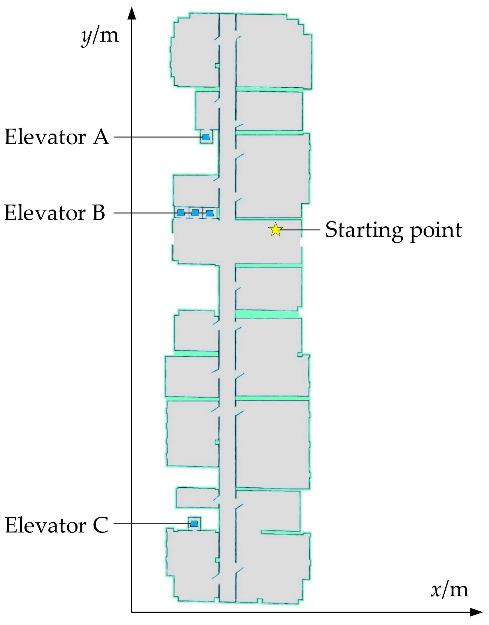
In this section, a typical business building Boyuan in North China University of Technology, Shijingshan District, Beijing, China, is selected as a real scenario to test the logistics system. The building consists of 11 floors with 300 rooms. A 3D coordinate system for the typical office building is established, as shown in Figure 9, where x and y are coordinates of plane positions and f is the floor coordinate. The origin of the coordinate system is set at the southwest corner of the building, which can ensure that all targets are positive in the coordinate system. The logistics center, with the coordinates (28.7, 55.2, 1), is set at the gate of the building, which is shown in Figure 10. The waiting time for customers to pick up the goods from the target is not included in the total distribution time. The intelligent elevator can be called to the designated floor in advance, so the waiting time of the elevator can be ignored.
In the distribution process, the current delivery mass will affect the speed of the actuator. However, limitations of speed at 2 m/s and acceleration at 1.75 m/s2 for actuator are set due to the risk of pedestrian safety. Therefore, in this actuator, there is enough power to meet the speed demand at full load. The distribution process of the experiment is shown in Figure 11.
In the experiment, delivery distance, delivery time and calculation time are selected as indexes. To better explain the meaning of experimental process and indexes, a scheme generated by A*+GAHC algorithm is selected as an example. There is one starting point, twenty target points and three sets of elevators in the example. Firstly, the delivery distance and delivery time between each two points of twenty-one points are calculated by A* algorithm. If they are on different floors, the delivery distance and delivery time of three different elevators to the target are calculated, which obtained a total of 584 pairs of data. Then, the distribution scheme is solved by the GAHC algorithm, which includes three delivery routes: “0-1-7-5-14-8-6-0”, “0-17-11-18-4-3-20-13-0” and “0-12-16-15-2-19-10-0”. Taking “0-1-7-5-14-8-6-0” as an example, the actuator departs from the starting point, delivers the targets numbered 1, 7, 5, 14, 8 and 6, and returns to the starting point. The calculation time is the time required to generate the scheme read by the timer. Finally, after distribution, the total distance and total time of distribution are obtained by reading the data of the odometer and timer.
Crossover rate and mutation rate, as the critical parameters of GA, affect the experimental results. Therefore, we try to explore the optimal values of them for the better performance. With the same scenes and targets, crossover rate is set up from 0.1 to 1.0, and mutation rate is defined as 0.1. The experimental results are shown in Table 1 and Figure 12.
As shown in Table 1 and Figure 12, the total delivery time fluctuates along with the change of crossover rate. It is obvious that when the cross rate is set up as 0.7, the delivery has the minimum of the total time. However, it has little effect for crossover rate on the calculation time of the GA. Because the crossover operation is of a significant concern to genetic operations, a crossover rate causing a major effect on the calculation time should be selected. Therefore, crossover rate 0.7 is selected for the experiment.
Similarly, mutation rate ranges from 0.1 to 1.0, and crossover rate is set as 0.7. The total delivery time and the calculation time are shown in Table 2 and Figure 13.
As shown in Table 2 and Figure 13, when mutation rate is set up within the range from 0.1 to 0.7, the total delivery time shows an upward trend, along with an increase in mutation rate. When mutation rate is set up to 0.8, the delivery time witnesses a downward trend. Moreover, the calculation time increases linearly with the increase in mutation rate. A higher mutation rate means that the algorithm tends to perform random searches. Therefore, in this paper, setting mutation rate to 0.1 is rational for the quality of the solution.
In order to realize indoor route planning based on SLAM rapidly, parameters of the algorithm are selected in Table 3, and the corresponding parameters to the targets are shown in Table 4.
For the purpose of verifying the effectiveness of this proposed algorithm (A*+GAHC), the traditional algorithms Dijkstra (Dijkstra+GAHC), BFS (BFS+GAHC), HC (A*+HC) and GA (A*+GA) are compared in the experiment. The above five algorithms are each tested 10 times, and the delivery times are shown in Table 5 and Figure 14.
As shown in Figure 14, the data of Dijkstra+GAHC, A*+HC, A*+GA and A*+GAHC are relatively stable and different from each other in the same environment and objectives. It should be noted that the data of BFS+GAHC fluctuate greatly. To analyze the experimental data more clearly, the four indexes including average delivery distance, average delivery time, standard deviation of solutions and average calculation time are analyzed. The results are shown in Table 6.
Time and energy cost are sensitive in logistics actuators. Therefore, the average delivery time and the average delivery distance are firstly selected for analysis. The average delivery time indicates the time cost of the intelligent system, and the average delivery distance reflects the energy cost of the actuator. Moreover, there is a correlation between the average delivery time and the average delivery distance in this experiment, as shown in Figure 15.
As revealed in Figure 15, the shortest average delivery time is achieved through Dijkstra+GAHC. The second shortest average delivery time is obtained by A*+GAHC, which is only 3.4% slower than that of Dijkstra+GAHC. It is worth noting that the longest average delivery time is gained by BFS+GAHC. The reasons can be analyzed as follows. Dijkstra+GAHC based on Dijkstra is a greedy strategy, which traverses all potential nodes through breadth first search. Therefore, Dijkstra+GAHC can find the optimal solution more accurately and stably. BFS-based BFS+GAHC can achieve the aim of single fastest delivery due to the tendency of goal orientations. However, BFS+GAHC may become stuck in the bilateral or multilateral traps, which leads to unstable and long delivery times. The A*+GA, A*+HC and A*+GAHC based on A* algorithm can ensure stability and make the solution approach the optimal solution of the problem. Moreover, A*+GA, A*+HC and A*+GAHC still have some differences in solving multi-objective distribution problems: A*+HC can find the optimal solution quickly in local through HC algorithm, A*+GA can analyze the problem globally by GA to ensure the stability of the solution and A*+GAHC combined with HC and GA can ensure the stability and rapidity of the solution, and its average delivery time is closer to the optimal solution than the performance of other algorithms.
Secondly, as an important index in the system, the average calculation time reflects the ability to replan the route for special situations encountered in the distribution process. Before the delivery of the logistics actuator, the system analyzes and calculates the distribution scheme for the environment. Therefore, the lower the index, the higher the robustness of the system. As shown in Figure 16, Dijkstra+GAHC based on Dijkstra algorithm requires a large amount of computation, which is about 30 times greater than other algorithms because it traverses all potential nodes. BFS+GAHC has a long calculation time for the tendency of the BFS algorithm to the target orientation. A*+GA, A*+HC and A*+GAHC, based on A*, have a relatively stable trend in calculation time. A*+HC based on HC has the fastest calculation time due to the fact that the global situation does not need to be considered. For A*+GA based on GA algorithm, more calculation time is allocated in the global solution process. A*+GAHC, combining HC and GA algorithm, has a strong robustness, and the calculation time is only 7% slower than the fastest delivery time through A*+GA.
In the total distribution process, the average time T is generally used as a main index, and its calculation equation is as Equation (12):
T = α t 1 + β t 2
where t1 is the average delivery time, t2 is the average calculation time and α and β are the weights related to calculate the average time.
In the process of this experiment, the distribution environment is relatively stable, and there is no need to replan calculation and redistribution. Therefore, the weights are set as Equation (13):
α = β = 1
As shown in Figure 17, the average time in Dijkstra+GAHC even surpasses the average time in A*+HC or A*+GAHC because it increases the calculation time. Compared with other algorithms, A*+GAHC proposed in this paper has an advantage of 22.7% in reducing average total time cost.
Thirdly, the standard deviation of solutions displays the stability of the algorithms. As shown in Figure 18, Dijkstra+GAHC has the strongest stability because it traverses all potential nodes. Due to the greed tendency, and the standard deviation in BFS+GAHC is generally higher than other algorithms. The algorithm A*+GAHC, combining GA and HC, has the smallest standard deviation and strong stability.
Five algorithms in the experiment have distinct characteristics. Moreover, these different characteristics in environments affect the experimental results to some extent, which is shown in Table 7.
Therefore, the following conclusions can be drawn from the above experimental analysis:
(1)
Dijkstra+GAHC has a strong analysis ability both locally and globally and can find the optimal solution in multi-objective distribution tasks. However, a large amount of data and long calculation times in the analysis of Dijkstra lead to poor robustness and long total time.
(2)
BFS+GAHC has the fastest single delivery time, but it takes a long time for calculation and has the poorest stability due to the randomness of the BFS algorithm.
(3)
A*+HC and A*+GA are near-optimal solutions in delivery time and can ensure shorter calculation times and strong stabilities at the same time. However, A*+HC, based on the local solving ability of the HC algorithm, still has some shortcomings in the multi-objective distribution problems. Similarly, A*+GA, based on the global solving ability of the GA algorithm, has the weakness of a long calculation time.
(4)
A*+GAHC proposed in this paper makes the delivery time approach the optimal solution through the A* algorithm, while ensuring less calculation time and a strong stability. Moreover, in multi-objective distribution problems, the integration of the HC and GA algorithms places the logistics system in an efficient and stable state.

4. Conclusions

Compared with outdoor logistics distribution based on high precision GPS, this paper designs and implements an intelligent wheeled actuator to improve the efficiency of indoor logistics distribution. The proposed system includes a wheeled actuator, intelligent elevators and a remote logistics center. Firstly, this paper proposed a novel multi-sensor fusion method which was applied to the intelligent actuator of an indoor logistics system. Then, through the SLAM method of multi-node interconnections based on a wireless communication network, the function of cross-floor route planning and distribution was realized. Finally, this paper proposed a novel A*+GAHC algorithm to improve the distribution efficiency of the actuator in an indoor logistics system. An advantage of 22.7% reduced average total time cost was confirmed by comparing A*+GAHC with other algorithms. Through the test in the real scenario, experimental results have shown that the wheeled actuator can improve the delivery efficiency and reduce the route planning time. The final delivery task by autonomous driving can be completed accurately. Therefore, with further technologies of AI and autonomous driving, more advanced scenarios and complex algorithms can be applied in our daily lives, and the labor costs in logistics system will be greatly reduced.

Author Contributions

Conceptualization, P.W. and J.Z.; methodology, Y.W.; software, Y.W.; validation, Y.W., X.W. and Y.L.; formal analysis, P.W.; investigation, P.W.; resources, P.W.; data curation, Y.W.; writing—original draft preparation, P.W. and Y.W.; writing—review and editing, J.Z.; visualization, P.W.; supervision, P.W.; project administration, P.W.; funding acquisition, P.W. All authors have read and agreed to the published version of the manuscript.

Funding

This research was funded by the Beijing Natural Science Foundation (Grant number 4212034) and National Key R&D Program of China (Grant number 2018YFB1600500).

Institutional Review Board Statement

Not applicable.

Informed Consent Statement

Not applicable.

Data Availability Statement

All data and models used during the study appear in this article.

Acknowledgments

The authors would like to thank X. Liu and C. Liu for their technical assistance with the experiments and analysis.

Conflicts of Interest

The authors declare no conflict of interest.

References

  1. Cousins, S. Exponential growth of ROS. IEEE Robot. Autom. Mag. 2011, 1, 19–20. [Google Scholar]
  2. Wang, P.; Jiang, Y.; Xiao, L.; Zhao, Y.; Li, Y. A joint control model for connected vehicle platoon and arterial signal coordination. J. Intell. Transp. Syst. 2020, 24, 81–92. [Google Scholar] [CrossRef]
  3. Raible, J.; Blaich, M.; Bittel, O. Differential GPS supported navigation for a mobile robot. IFAC Proc. Vol. 2010, 43, 318–323. [Google Scholar] [CrossRef] [Green Version]
  4. Khaliq, A.A.; Di Rocco, M.; Saffiotti, A. Stigmergic algorithms for multiple minimalistic robots on an RFID floor. Swarm Intell. 2014, 8, 199–225. [Google Scholar] [CrossRef]
  5. Davison, A.J.; Cid, Y.G.; Kita, N. Real-time 3d SLAM with wide-angle vision. IFAC Proc. Vol. 2004, 37, 868–873. [Google Scholar] [CrossRef]
  6. Blanco, J.; Fernández-Madrigal, J.; Gonzalez, J. A Novel Measure of Uncertainty for Mobile Robot SLAM with Rao-Blackwellized Particle Filters. Int. J. Robot. Res. 2008, 27, 73–89. [Google Scholar] [CrossRef]
  7. Rajam, C.; Roopsingh, D. Optimal Parameter Analysis of Two 2D Lidar SLAM. Vet. Nurse 2014, 1. [Google Scholar]
  8. Vlaminck, M.; Luong, H.; Philips, W. Have I seen this place before? A fast and robust loop detection and correction method for 3D lidar SLAM. Sensors 2018, 19, 23. [Google Scholar] [CrossRef] [PubMed] [Green Version]
  9. Wang, P.; Wang, Y.; Deng, H.; Zhang, M.; Zhang, J. Multilane Spatiotemporal Trajectory Optimization Method (MSTTOM) for Connected Vehicles. J. Adv. Transp. 2020. [Google Scholar] [CrossRef]
  10. Barzdins, J.; Kirikova, M.; Vaira, G. Parallel bidirectional Dijkstra’s shortest path algorithm. Front. Artif. Intell. Appl. 2011, 224, 422–435. [Google Scholar]
  11. Sierra, M.R. Improving heuristic search algorithms by means of pruning by dominance. Application to scheduling problems. AI Commun. 2013, 26, 323–324. [Google Scholar] [CrossRef]
  12. Ducho, Ė.F.; Babineca, A.; Kajana, M. Path planning with modified a star algorithm for a mobile robot. Procedia Eng. 2014, 96, 59–69. [Google Scholar] [CrossRef] [Green Version]
  13. Chedjou, J.C.; Kyamakya, K. Benchmarking a recurrent neural network based efficient shortest path problem (SPP) solver concept under difficult dynamic parameter settings conditions. Neurocomputing 2016, 196, 175–209. [Google Scholar] [CrossRef]
  14. Elhoseny, M.; Shehab, A.; Yuan, X. Optimizing robot path in dynamic environments using Genetic Algorithm and Bezier Curve. J. Intell. Fuzzy Syst. 2017, 33, 2305–2316. [Google Scholar] [CrossRef] [Green Version]
  15. Dewang, H.S.; Mohanty, P.K.; Kundu, S. A Robust Path Planning for Mobile Robot Using Smart Particle Swarm Optimization. Procedia Comput. Sci. 2018, 133, 290–297. [Google Scholar] [CrossRef]
  16. Wang, P.; Deng, H.; Zhang, J.; Wang, L.; Zhang, M.; Li, Y. Model predictive control for connected vehicle platoon under switching communication topology. IEEE Trans. Intell. Transp. Syst. 2021. [Google Scholar] [CrossRef]
  17. Rosenthal, S.; Veloso, M. Mobile robot planning to seek help with spatially-situated tasks. In Proceedings of the Twenty-Sixth AAAI Conference on Artificial Intelligence, Toronto, ON, Canada, 22 July 2012. [Google Scholar]
  18. Zhang, J.; Wu, Y.; Min, G.; Hao, F.; Cui, L. Balancing energy consumption and reputation gain of uav scheduling in edge computing. IEEE Trans. Cogn. Commun. Netw. 2020, 6, 1204–1217. [Google Scholar] [CrossRef]
  19. Purian, F.K.; Sadeghian, E. Mobile robots path planning using ant colony optimization and Fuzzy Logic algorithms in unknown dynamic environments. In Proceedings of the 2013 International Conference on Control, Automation, Robotics and Embedded Systems, Jabalpur, India, 16–18 December 2013. [Google Scholar]
  20. Abdulla, A.A.; Liu, H.; Stoll, N. Multi-floor navigation method for mobile robot transportation based on StarGazer sensors in life science automation. In Proceedings of the 2015 IEEE International Instrumentation and Measurement Technology Conference Proceedings, Pisa, Italy, 11–14 May 2015. [Google Scholar]
  21. Bae, J.; Chung, W. A heuristic for a heterogeneous automated guided vehicle routing problem. Int. J. Precis. Eng. Manuf. 2017, 18, 795–801. [Google Scholar] [CrossRef]
  22. Mosallaeipour, S.; Najad, M.G.; Shavarani, S.M. Mobile robot scheduling for cycle time optimization in flow-shop cells, a case study. Prod. Eng. 2018, 12, 83–94. [Google Scholar] [CrossRef]
  23. Khosiawan, Y.; Khalfay, A.; Nielsen, I. Scheduling unmanned aerial vehicle and automated guided vehicle operations in an indoor manufacturing environment using differential evolution-fused particle swarm optimization. Int. J. Adv. Robot. Syst. 2018, 15. [Google Scholar] [CrossRef]
  24. Szegedy, C.; Alexander, T.; Dumitru, E. Deep neural networks for object detection. Adv. Neural Inf. Process. Syst. 2013, 26. [Google Scholar]
  25. Dwijotomo, A.; Abdul Rahman, M.A.; Mohammed Ariff, M.H.; Zamzuri, H.; Wan Azree, W.M.H. Cartographer SLAM method for optimization with an adaptive multi-distance scan scheduler. Appl. Sci. 2020, 10, 347. [Google Scholar] [CrossRef] [Green Version]
  26. Dordaie, N.; Navimipour, N.J. A hybrid particle swarm optimization and hill climbing algorithm for task scheduling in the cloud environments. ICT Express 2018, 4, 199–202. [Google Scholar] [CrossRef]
Figure 1. The system structure of the wheeled autonomous actuator of logistics system.
Actuators 10 00120 g001
Figure 2. The flow of the ROS platform.
Actuators 10 00120 g002
Figure 3. Flowchart of data fusion.
Actuators 10 00120 g003
Figure 4. An example of collision avoidance.
Actuators 10 00120 g004
Figure 5. The flow chart of collision avoidance and overtaking.
Actuators 10 00120 g005
Figure 6. The framework of simultaneous localization and mapping (SLAM).
Actuators 10 00120 g006
Figure 7. An initial map of a laboratory as an example built by SLAM.
Actuators 10 00120 g007
Figure 8. The flowchart of the indoor route planning.
Actuators 10 00120 g008
Figure 9. The tested scenario in Beijing.
Actuators 10 00120 g009
Figure 10. Schematic diagram of starting point position.
Actuators 10 00120 g010
Figure 11. The distribution process of the experiment.
Actuators 10 00120 g011
Figure 12. Influence of crossover rate on GA.
Actuators 10 00120 g012
Figure 13. Influence of mutation rate on GA.
Actuators 10 00120 g013
Figure 14. Delivery time in various algorithms.
Actuators 10 00120 g014
Figure 15. Average delivery time and average delivery distance in various algorithms.
Actuators 10 00120 g015
Figure 16. Average calculation time in various algorithms.
Actuators 10 00120 g016
Figure 17. Average total time in various algorithms.
Actuators 10 00120 g017
Figure 18. Standard deviation of solutions in various algorithms.
Actuators 10 00120 g018
Table 1. Influence of crossover rate on GA.
Crossover RateTotal Distance (m)Total Time (min)Calculation Time (s)
0.11956.443.87.20
0.21615.643.87.50
0.31632.944.96.62
0.41624.543.87.30
0.51632.344.96.96
0.61623.543.87.56
0.71624.942.67.31
0.81650.643.86.80
0.91641.744.97.61
1.01626.943.87.11
Table 2. Influence of mutation rate on GA.
Mutation RateTotal Distance (m)Total Time (min)Calculation Time (s)
0.11624.942.67.31
0.21868.048.514.81
0.31875.950.921.16
0.41747.547.331.72
0.51885.150.932.44
0.61797.546.248.30
0.71850.149.753.08
0.81596.041.479.54
Table 3. Related parameters of the indoor route planning algorithm.
ParametersValuesSymbols
Population size20L
Crossover rate0.7Pc
Mutation rate0.1Pm
Gene exchange times5J
Penalty weight (minutes)100Pw
Hill climbing exchange times25Ph
Maximum iteration times300Pn
Local maximum iteration times50Pt
Maximum speed2vmax
Maximum acceleration1.75umax
Maximum delivery load8Q
Table 4. Parameters of targets.
Targets x (m)y (m)f (Floor)q (kg)
119.242.511.5
227.617.070.4
323.183.281.7
428.476.051.5
523.358.121.7
64.443.390.9
723.938.020.8
820.942.771.3
926.810.581.2
1020.726.290.4
1110.084.531.3
1222.213.011.3
132.743.5110.6
1425.555.631.5
1519.15.261.7
160.314.731.9
1728.899.020.1
1827.875.541.6
199.628.081.1
2022.474.881.2
Table 5. Delivery time (minutes) in various algorithms.
No.Djistra+GAHCBFS+GAHCA*+HCA*+GAA*+GAHC
141.782.748.247.643.0
242.453.742.348.443.4
340.2101.242.947.342.2
440.663.441.547.044.0
541.067.850.348.941.5
640.770.941.748.242.5
741.862.046.949.242.4
841.249.742.650.340.8
940.775.244.346.141.8
1041.067.941.349.243.7
Table 6. Comparison of results after calculated in various algorithms.
AlgorithmAverage Delivery Distance (m)Average Delivery Time (min)Standard Deviation of SolutionsAverage Calculation Time (s)
Dijkstra+GAHC1597.341.10.63309.62
BFS+GAHC2712.369.714.7316.36
A*+HC1684.544.23.016.82
A*+GA1767.648.21.1811.62
A*+GAHC1624.742.50.967.31
Table 7. Main characteristics and environments that impact the effects of each algorithm.
AlgorithmsMain CharacteristicsEnvironments that Impact the Effects
Dijkstra+GAHCThe most accurate analysis, but the longest computing time.A large number of nodes.
BFS+GAHCThe fastest analysis, but poor stability and effects.Traps between nodes.
A*+HCThe fastest time to find the local optimal solution, but unstable global solutions.Wide distribution of global solutions.
A*+GAThe fastest time to find the global optimal solution range, but the local optimal solution cannot be locked.Monotonic global solution.
A*+GAHCThe best effect, the strongest robustness and both global and local optimal solutions are considered.Complex algorithm design.
Publisher’s Note: MDPI stays neutral with regard to jurisdictional claims in published maps and institutional affiliations.

