
Electromagnetic Actuator System Using Witty Control System

Abstract
1. Introduction
2. Materials
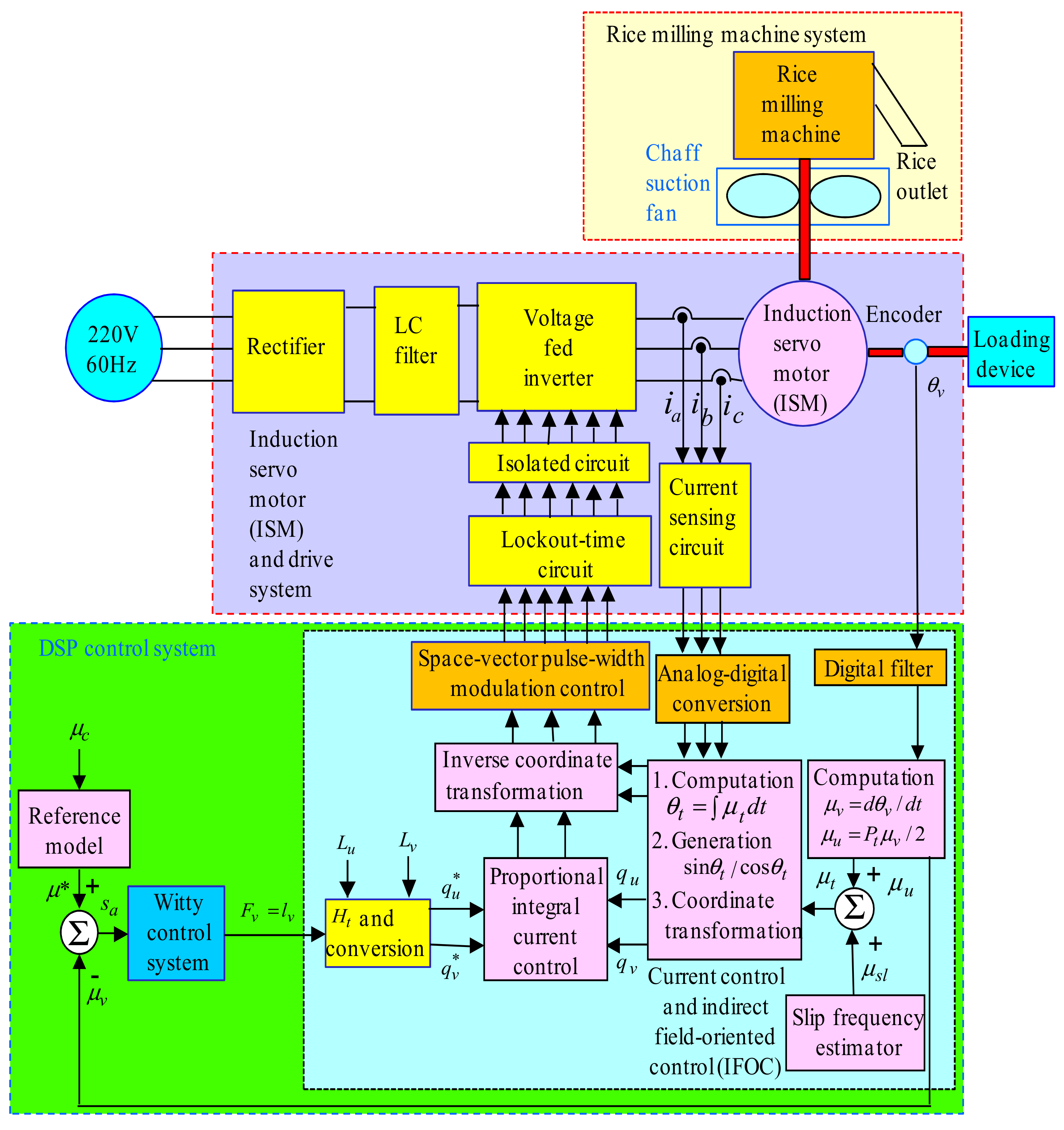
2.1. System Description
2.2. System Model
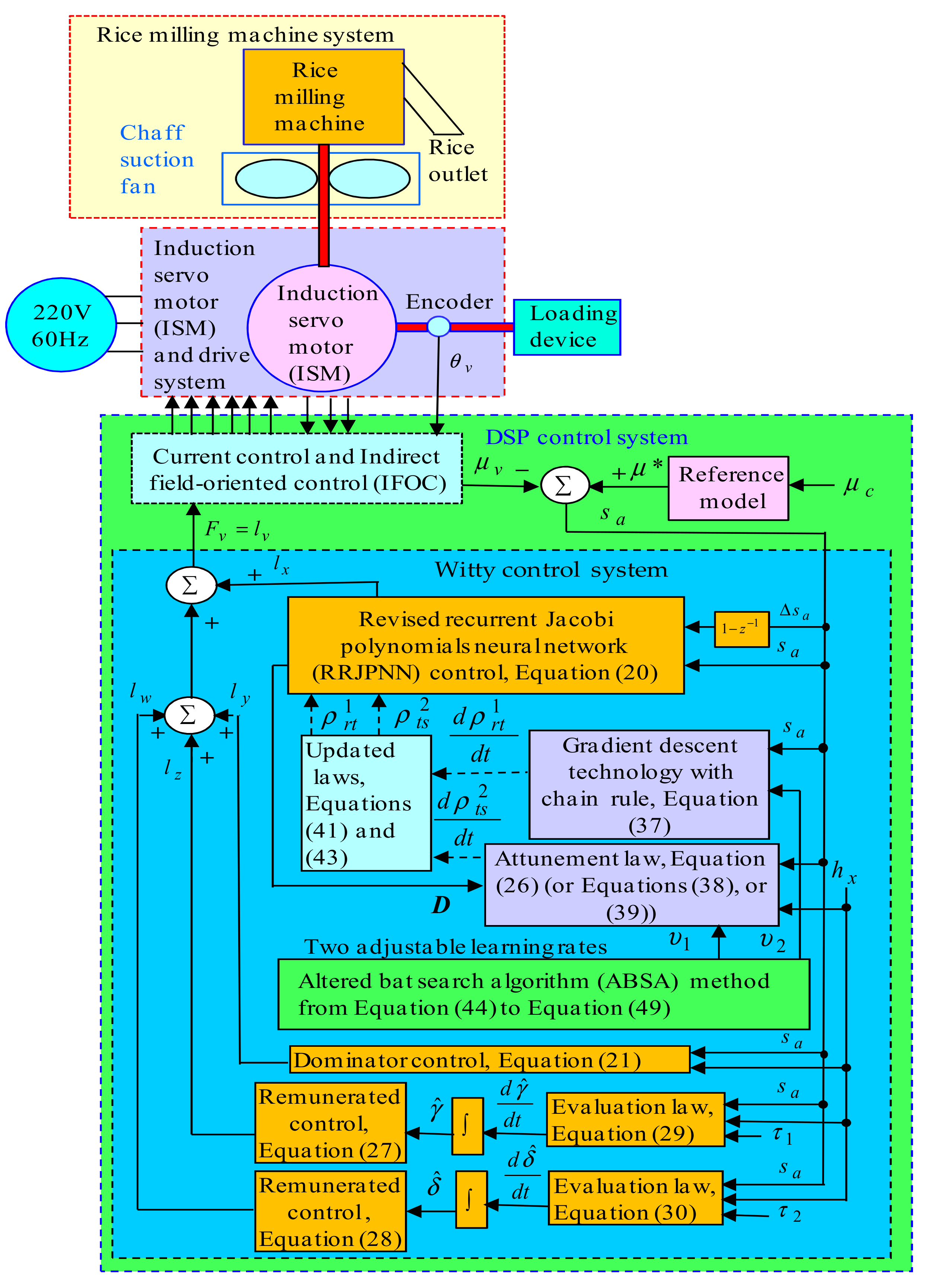
3. Methods
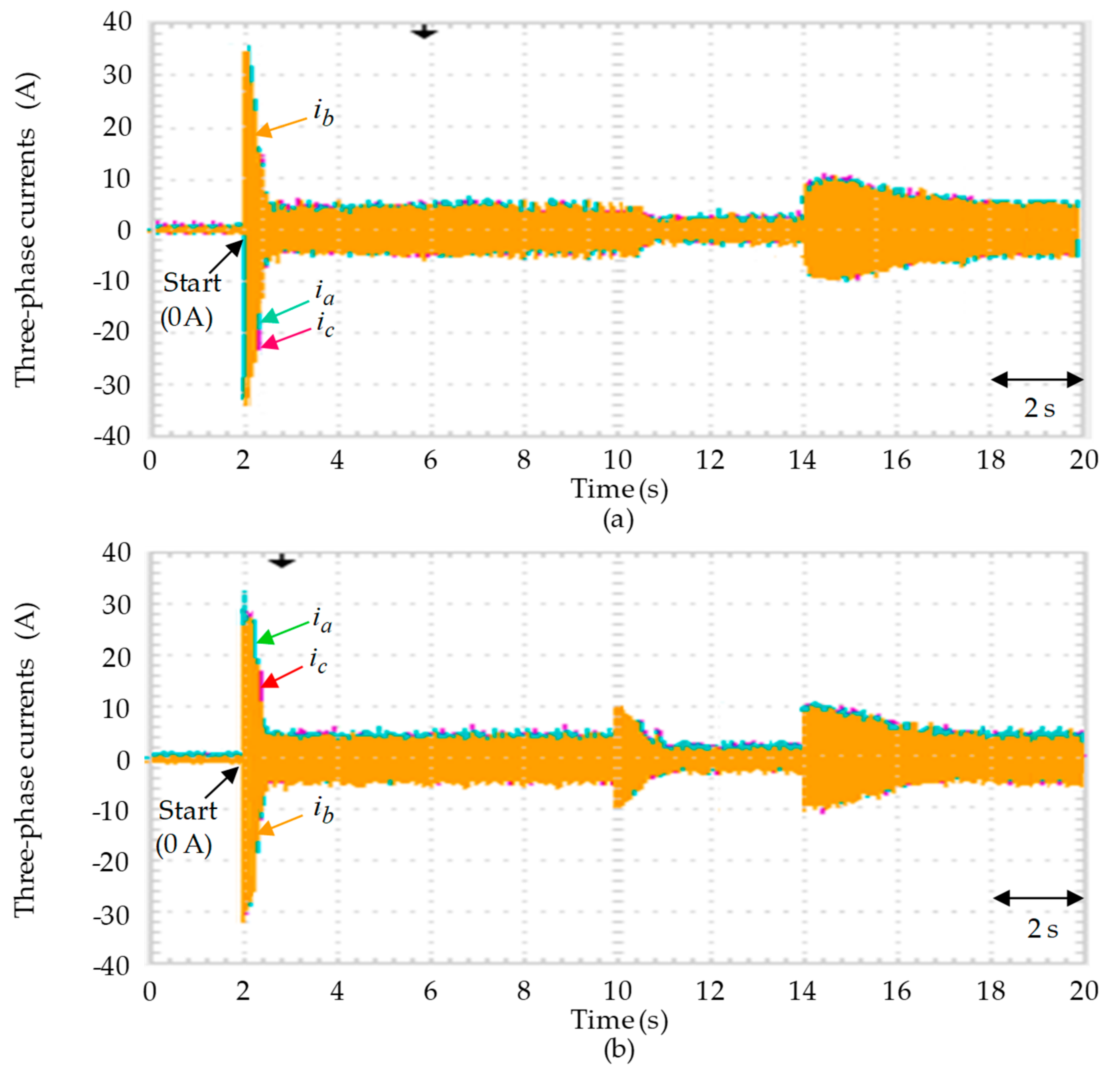
4. Tests and Results
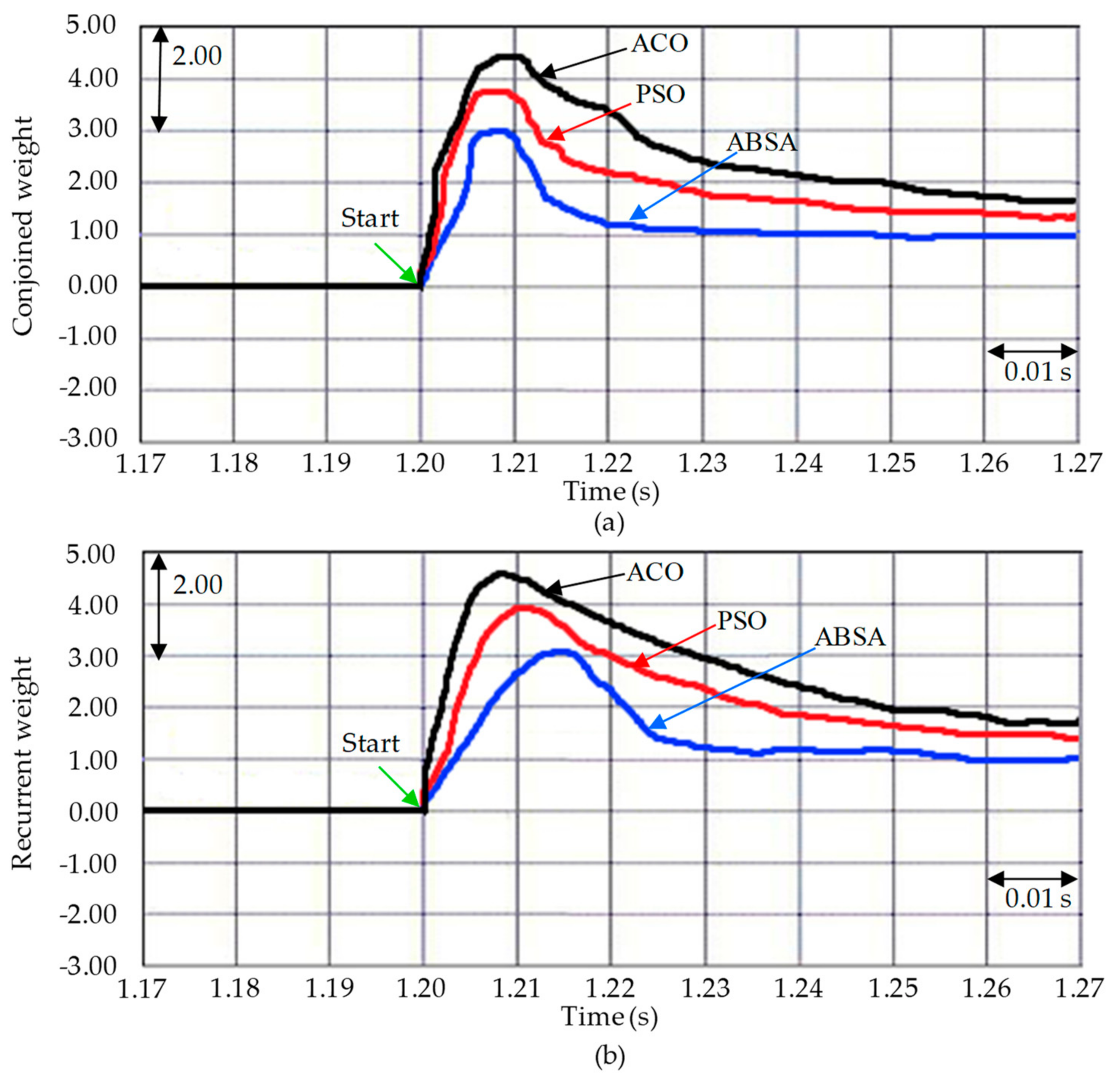
5. Analyses and Discussion
6. Conclusions
Author Contributions
Funding
Institutional Review Board Statement
Informed Consent Statement
Data Availability Statement
Conflicts of Interest
Abbreviations
| , | axis stator voltages |
| , | axis stator currents |
| , | axis rotor currents |
| , , | axis self inductances, mutual inductance |
| , | stator and equalized rotor resistances. |
| , , | mechanical and electrical angular speeds, electrical angular speed of synchronous flux in the ISM |
| electromagnetic torque | |
| , | axis flux linkages |
| number of pole | |
| , , | electromagnetic torque of the ISM, the output torque of idler 2 and the output torque of the main idler |
| , , , | four moments of inertia in the ISM, in idler 2, in the main idler and in idler 1 |
| , , , | four viscid frictional coefficients in the ISM, in idler 2, in the main idler and in idler 1 |
| transposition ratios regarding idler 2 and the main idler for the rice milling machine system | |
| nonlinear coalescence disturbances function | |
| , , | rolling force, wind force, braking force |
| , | speed in idler 2 and the speed in the main idler. |
| coalescence viscid friction coefficient including the main idler and the ISM | |
| coalescence moment of inertia including the main idler and the ISM | |
| huge comprehensive coalescence disturbances and parameter variations | |
| coalescence torque | |
| , , | coulomb friction torque, Stribeck effect torque, adding load torque |
| comprehensive coalescence disturbances | |
| comprehensive parameter variations | |
| comprehensive coalescence disturbances | |
| friendly ratio constant | |
| bounded with functional-bounded value | |
| friendly constant concerning the coalescence moment of inertia | |
| friendly constant concerning the coalescence moment of inertia | |
| , | two friendly values with bound |
| electromagnetic torque of the ISM | |
| speed difference | |
| positive control gain | |
| , , , | RRJPNN control, dominator control, two remunerated controls |
| , | speed difference alteration, speed difference |
| , and | node number of the center layer, the recurrent gain of the center layer and the iteration number |
| , | recurrent weight, conjoined weight |
| , , | three linear activation functions in the forehead, center and readward layers |
| , , | information of three outputs of nodes in the forehead, center and readward layers |
| Jacobi polynomial function | |
| , , | 0-, 1- and 2-order Jacobi polynomial functions |
| output information in the readward layer | |
| , | input information and weight vectors in the readward layer |
| minimum difference | |
| excellent control rule of the RRJPNN control | |
| excellent weight vector | |
| greater than zero real number | |
| uniformly continuous function | |
| , | two bounded |
| sign function | |
| objective function | |
| attunement law | |
| , | learning rate of the conjoined weight, learning rate of the recurrent weight |
| , | two positive evaluation rates |
| , | two evaluation differences |
| , | two evaluation laws |
| , | position of the bat i at n − 1 time, flight velocity of the bat i at n − 1 time |
| , | position of the bat i at n time, flight velocity of the bat i at n time |
| current global optimal position | |
| maximum number of iterations | |
| , | maximum and minimum frequencies of the soundwaves produced by the bat |
| random number at [−1, 1] | |
| solution selected from the current optimal solution at n − 1 time | |
| average loudness from the bat generation at n time | |
| , | modified loudness at n + 1 time, modified pulse rate at n + 1 time |
| , | initial rate, initial loudness |
| , | constant between 0 and 1, positive constant |
References
- Zuo, L.; Cheng, T.; Zuo, J.; Liu, Y.; Yang, S. A hierarchical intelligent control system for milling machine. In Proceedings of the IEEE International Conference on Intelligent Processing Systems, Beijing, China, 28–31 October 1997; pp. 1–6. [Google Scholar]
- Huang, S.; Tan, K.K.; Hang, G.S.; Wang, Y.S. Cutting force control of milling machine. Mechatronics 2007, 17, 533–541. [Google Scholar] [CrossRef]
- Lobinho, G.; Armando, S. Control of milling machine cutting force using artificial neural networks. In Proceedings of the 6th Iberian Conference on Information Systems and Technologies (CISTI 2011), Chaves, Portugal, 15–18 June 2011; pp. 1–6. [Google Scholar]
- Tadeusz, M. Numerical control system of conventional milling machine. Appl. Mech. Mater. 2016, 841, 179–183. [Google Scholar]
- Tu, F.; Hu, S.; Zhuang, Y.; Lv, J.; Wang, Y.; Sun, Z. Hysteresis curve fitting optimization of magnetic controlled shape memory alloy actuator. Actuators 2016, 5, 25. [Google Scholar] [CrossRef]
- Nakshatharan, S.S.; Vunder, V.; Poldsalu, I.; Johanson, U.; Punning, A.; Aabloo, A. Modelling and control of ionic electroactive polymer actuators under varying humidity conditions. Actuators 2018, 7, 7. [Google Scholar] [CrossRef]
- Xia, B.; Miriyev, A.; Trujillo, C.; Chen, N.; Cartolano, M.; Vartak, S.; Lipson, H. Improving the actuation speed and multi-cyclic actuation characteristics of silicone/ethanol soft actuators. Actuators 2020, 9, 62. [Google Scholar] [CrossRef]
- Lee, T.; Kim, I. Design of a 2DOF ankle exoskeleton with a polycentric structure and a bi-directional tendon-driven actuator controlled using a PID neural network. Actuators 2021, 10, 9. [Google Scholar] [CrossRef]
- Wang, L.; Duan, M.; Duan, S. Memristive Chebyshev neural network and its applications in function approximation. Math. Probl. Eng. 2013, 2013, 1–7. [Google Scholar] [CrossRef]
- Ting, J.C.; Chen, D.F. Novel mingled reformed recurrent hermite polynomial neural network control system applied in continuously variable transmission system. J. Mech. Sci. Technol. 2018, 32, 4399–4412. [Google Scholar] [CrossRef]
- Soltani, M.; Hegde, C. Fast and provable algorithms for learning two-layer polynomial neural networks. IEEE Trans. Signal Process. 2019, 67, 3361–3371. [Google Scholar] [CrossRef]
- Ting, J.C.; Chen, D.F. Nonlinear backstepping control of SynRM drive systems using reformed recurrent Hermite polynomial neural networks with adaptive law and error estimated law. J. Power Electron. 2018, 8, 1380–1397. [Google Scholar]
- Richard, A.; James, W. Some Basic Hypergeometric Orthogonal Polynomials that Generalize Jacobi Polynomials; American Mathematical Soc.: Providence, RI, USA, 1985; p. 54. [Google Scholar]
- Guo, B.Y.; Shen, J.; Wang, L.L. Generalized Jacobi polynomials/functions and their applications. Appl. Numer. Math. 2009, 59, 1011–1028. [Google Scholar] [CrossRef]
- Rubio, J.J.; Yu, W. Nonlinear system identification with recurrent neural networks and dead-zone Kalman filter algorithm. Neurocomputing 2007, 70, 2460–2466. [Google Scholar] [CrossRef]
- Chen, D.F.; Shih, Y.C.; Li, S.C.; Chen, C.T.; Ting, J.C. Mixed modified recurring Rogers-Szego polynomials neural network control with mended grey wolf optimization applied in SIM expelling system. Mathematics 2020, 8, 754. [Google Scholar] [CrossRef]
- Abbasvandi, Z.; Nasrabadi, A.M. A self-organized recurrent neural network for estimating the effective connectivity and its application to EEG data. Comput. Biol. Med. 2019, 110, 93–107. [Google Scholar] [CrossRef]
- Park, K.; Kim, J.; Lee, J. Visual field prediction using recurrent neural network. Sci. Rep. 2019, 9, 8385. [Google Scholar] [CrossRef]
- Jaddi, N.S.; Abdullah, S.; Hamdan, A. Multi-population cooperative bat algorithm-based optimization of artificial neural network model. Inf. Sci. 2015, 294, 628–644. [Google Scholar] [CrossRef]
- Wang, L.; Geng, H.; Liu, P.; Lu, K.; Kolodziej, J.; Ranjan, R.; Zomaya, A.Y. Particle swarm optimization based dictionary learning for remote sensing big data. Knowl. Based Syst. 2015, 79, 43–50. [Google Scholar] [CrossRef]
- Liu, Z.Z.; Chu, D.H.; Song, C.; Xue, X.; Lu, B.Y. Social learning optimization (SLO) algorithm paradigm and its application in QoS-aware cloud service composition. Inf. Sci. 2016, 326, 315–333. [Google Scholar] [CrossRef]
- Wu, D.; Xu, S.; Kong, F. Convergence analysis and improvement of the chicken swarm optimization algorithm. IEEE Access 2016, 4, 9400–9412. [Google Scholar] [CrossRef]
- Gheraibia, Y.; Djafri, K.; Krimou, H. Ant colony algorithm for automotive safety integrity level allocation. Appl. Intell. 2017, 8, 555–569. [Google Scholar] [CrossRef]
- Yang, X.S. A new metaheuristic bat-inspired algorithm. In Nature Inspired Cooperative Strategies for Optimization (NICSO 2010); Springer: Berlin, Heidelberg, 2010; Volume 284, pp. 65–74. [Google Scholar]
- Adarsh, B.A.; Raghunathan, T.; Jayabarathi, T.; Yang, X.S. Economic dispatch using chaotic bat algorithm. Energy 2016, 96, 666–675. [Google Scholar] [CrossRef]
- Wang, Y.; Wang, P.; Zhang, J.; Cui, H.; Cai, X.; Zhang, W.; Chen, J. A novel bat algorithm with multiple strategies coupling for numerical optimization. Mathematics 2019, 7, 135. [Google Scholar] [CrossRef]
- Chen, D.F.; Cheng, A.B.; Chiu, S.P.C.; Ting, J.C. Electromagnetic torque control for six-phase induction motor expelled continuously variable transmission clumped system using sage dynamic control system. Int. J. Appl. Electromagn. Mech. 2021, 65, 579–608. [Google Scholar] [CrossRef]
- Singh, G.K.; Nam, K.; Lim, S.K. A simple indirect field oriented control scheme for multiphase induction machine. IEEE Trans. Ind. Electron. 2005, 52, 1117–1184. [Google Scholar] [CrossRef]
- Guo, Z.; Zhang, J.; Sun, Z.; Zheng, C. Indirect field oriented control of three-phase induction motor based on current-source inverter. Procedia Eng. 2017, 174, 588–594. [Google Scholar] [CrossRef]
- Han, Y.; Jia, F.; Zeng, Y.; Cao, B. Effects of rotation speed and outlet opening on particle flow in a vertical rice mill. Powder Technol. 2016, 297, 153–164. [Google Scholar] [CrossRef]
- Zareiforoush, H.; Minaee, S.; Alizadeh, M.R.; Samani, B.H. Design, development and performance evaluation of an automatic control system for rice whitening machine based on computer vision and fuzzy logic. Comput. Electron. Agric. 2016, 124, 14–22. [Google Scholar] [CrossRef]
- Ruekkasaem, L.; Sasananan, M. Optimal parameter design of rice milling machine using design of experiment. Mater. Sci. Forum 2018, 911, 107–111. [Google Scholar] [CrossRef]
- Astrom, K.J.; Hagglund, T. PID Controller: Theory, Design, and Tuning; Instrument Society of America: Research Triangle Park, NC, USA, 1995. [Google Scholar]
- Hagglund, T.; Astrom, K.J. Revisiting the Ziegler-Nichols tuning rules for PI control. Asian J. Control 2002, 4, 364–380. [Google Scholar] [CrossRef]
- Hagglund, T.; Astrom, K.J. Revisiting the Ziegler-Nichols tuning rules for PI control-part II: The frequency response method. Asian J. Control 2004, 6, 469–482. [Google Scholar] [CrossRef]
- Astrom, K.J.; Wittenmark, B. Adaptive Control; Addison-Wesley: New York, NY, USA, 1995. [Google Scholar]
- Slotine, J.J.E.; Li, W. Applied Nonlinear Control; Prentice-Hall: Englewood Cliffs, NJ, USA, 1991. [Google Scholar]
- Chen, D.F.; Shih, Y.C.; Li, S.C.; Chen, C.T.; Ting, J.C. Permanent-magnet SLM drive system using AMRRSPNNB control system with DGWO. Energies 2020, 13, 2914. [Google Scholar] [CrossRef]


| Controllers | TA Controller | TB Controller | ||||
|---|---|---|---|---|---|---|
| Performance | Maximum Differences of | Quadratic Mean Differences of | Maximum Differences of | Quadratic Mean Differences of | ||
| Three Test Examples | ||||||
| Test JA | 82 rpm | 48 rpm | 30 rpm | 17 rpm | ||
| (8.58 rad/s) | (5.02 rad/s) | (3.14 rad/s) | (1.78 rad/s) | |||
| Test JB | 128 rpm | 53 rpm | 35 rpm | 19 rpm | ||
| (13.40 rad/s) | (5.55 rad/s) | (3.66 rad/s) | (1.99 rad/s) | |||
| Test JC | 489 rpm | 188 rpm | 192 rpm | 46 rpm | ||
| (51.18 rad/s) | (19.68 rad/s) | (20.10 rad/s) | (4.81 rad/s) | |||
| Controllers | TA Controller | TB Controller | |
|---|---|---|---|
| Peculiarity Performances | |||
| Total harmonic distortion (THD) values in the three-phase currents in test JB | 21% | 5% | |
| Responses of rising times in test JB | 0.92 s | 0.75 s | |
| Regulation capabilities with adding load torque in test JC | 489 rpm (51.18 rad/s) in maximum difference | 192 rpm (20.10 rad/s) in maximum difference | |
| Speed tracking differences in test JB | 128 rpm (13.40 rad/s) in maximum difference | 35 rpm (3.66 rad/s) in maximum difference | |
| Denial potentialities of parameter disturbance in test JB | 128 rpm (13.40 rad/s) in maximum difference | 35 rpm (3.66 rad/s) in maximum difference | |
Publisher’s Note: MDPI stays neutral with regard to jurisdictional claims in published maps and institutional affiliations. |
© 2021 by the authors. Licensee MDPI, Basel, Switzerland. This article is an open access article distributed under the terms and conditions of the Creative Commons Attribution (CC BY) license (http://creativecommons.org/licenses/by/4.0/).
Share and Cite
Chen, D.-F.; Chiu, S.-P.-C.; Cheng, A.-B.; Ting, J.-C. Electromagnetic Actuator System Using Witty Control System. Actuators 2021, 10, 65. https://doi.org/10.3390/act10030065
Chen D-F, Chiu S-P-C, Cheng A-B, Ting J-C. Electromagnetic Actuator System Using Witty Control System. Actuators. 2021; 10(3):65. https://doi.org/10.3390/act10030065
Chicago/Turabian StyleChen, Der-Fa, Shen-Pao-Chi Chiu, An-Bang Cheng, and Jung-Chu Ting. 2021. "Electromagnetic Actuator System Using Witty Control System" Actuators 10, no. 3: 65. https://doi.org/10.3390/act10030065
APA StyleChen, D.-F., Chiu, S.-P.-C., Cheng, A.-B., & Ting, J.-C. (2021). Electromagnetic Actuator System Using Witty Control System. Actuators, 10(3), 65. https://doi.org/10.3390/act10030065