Author Contributions
Conceptualization, H.L.; methodology, H.L., L.W., K.Y., W.M., and J.W.; theoretical analysis, L.W. and K.Y.; validation, L.W., W.M., and J.W.; writing—original draft preparation, L.W.; writing—review and editing, H.L. and W.Z.; and funding acquisition, H.L. All authors have read and agreed to the published version of the manuscript.
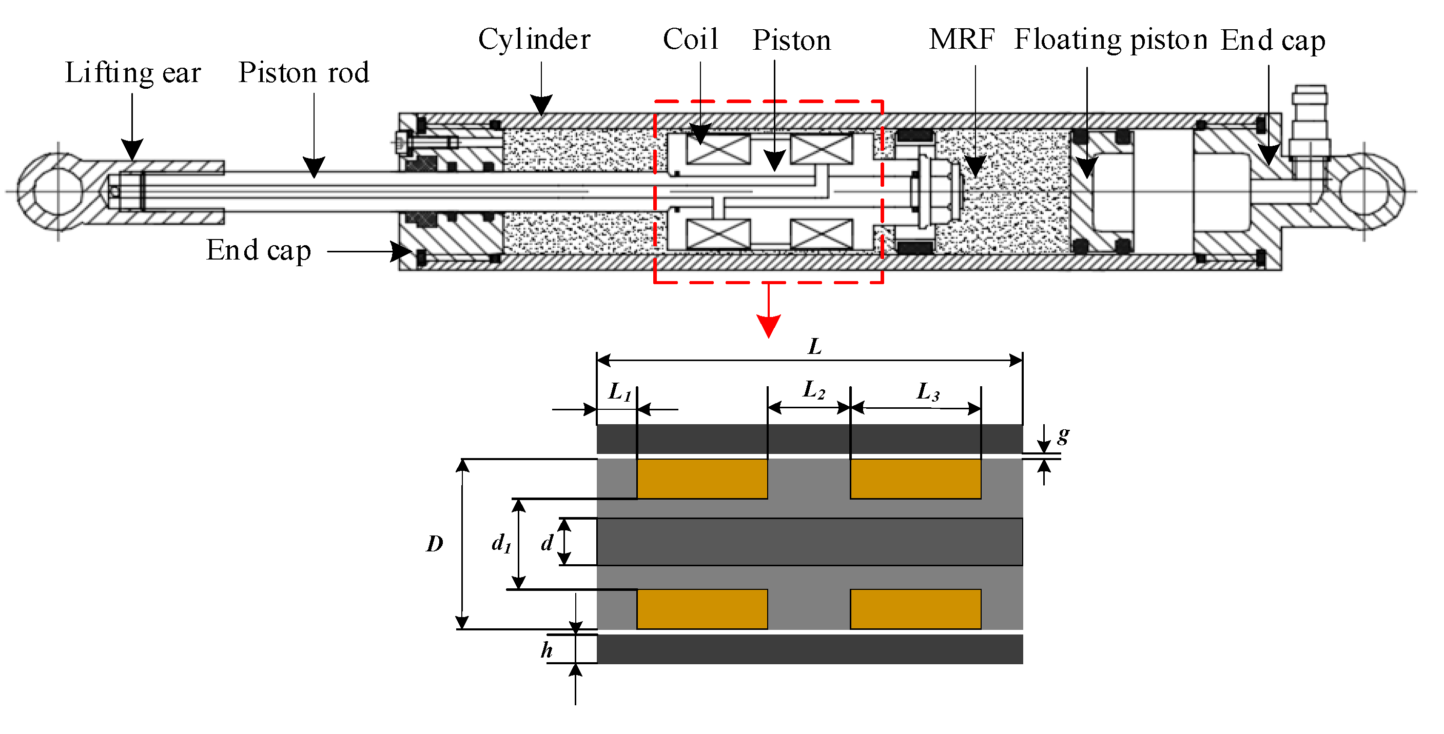
Figure 1.
A typical device of MRD.
Figure 1.
A typical device of MRD.
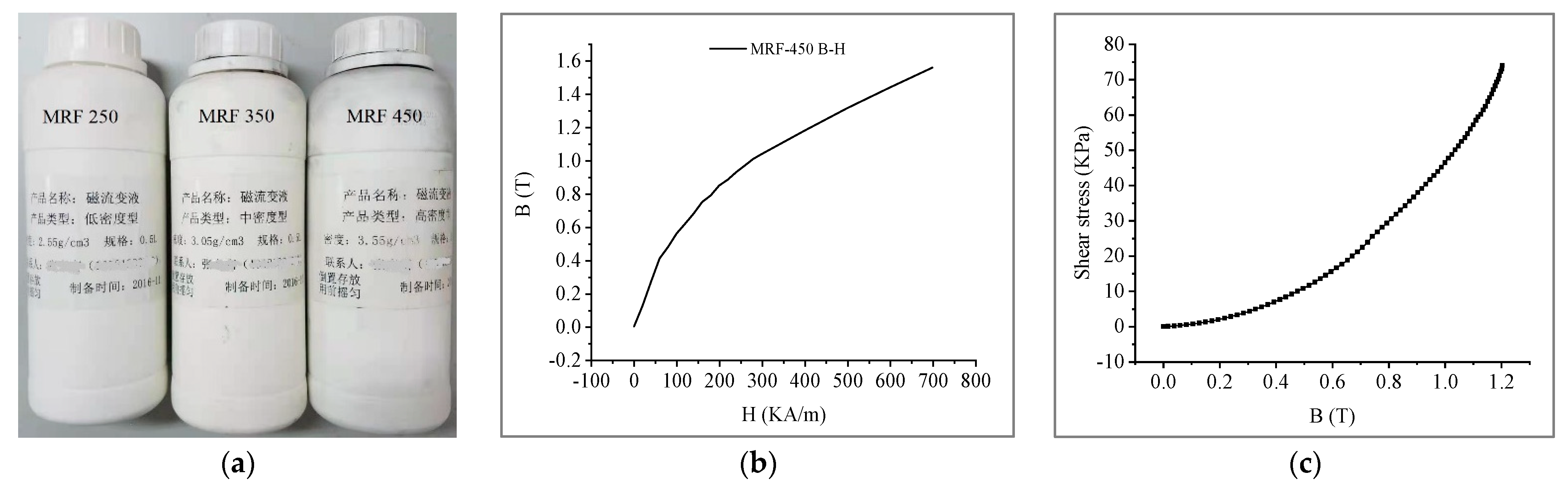
Figure 2.
MRF450: (a) description of MRF; (b) magnetization curve; and (c) the shear stress vs. magnetic induction intensity.
Figure 2.
MRF450: (a) description of MRF; (b) magnetization curve; and (c) the shear stress vs. magnetic induction intensity.
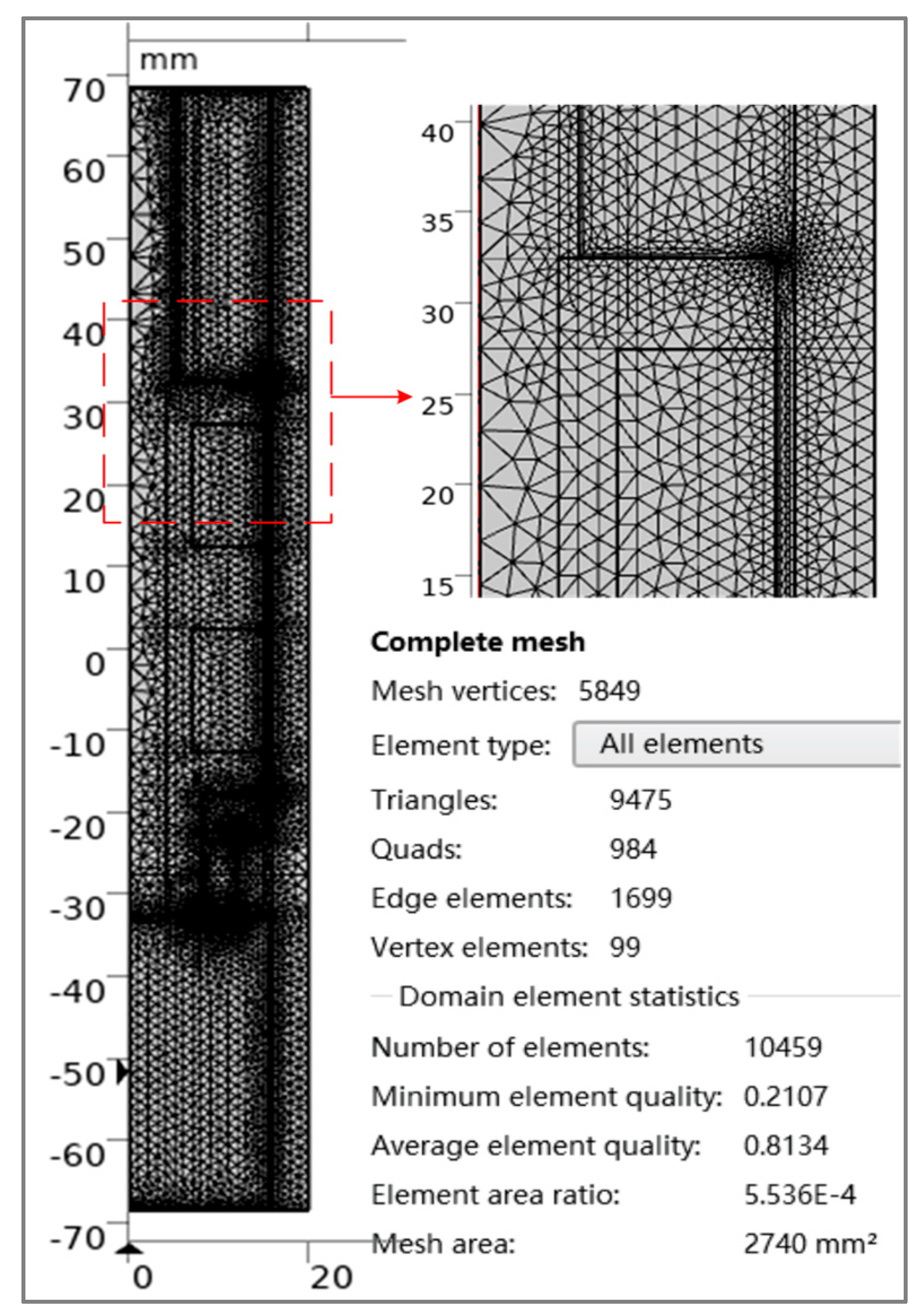
Figure 3.
The finite-element mesh for the two-dimensional model.
Figure 3.
The finite-element mesh for the two-dimensional model.
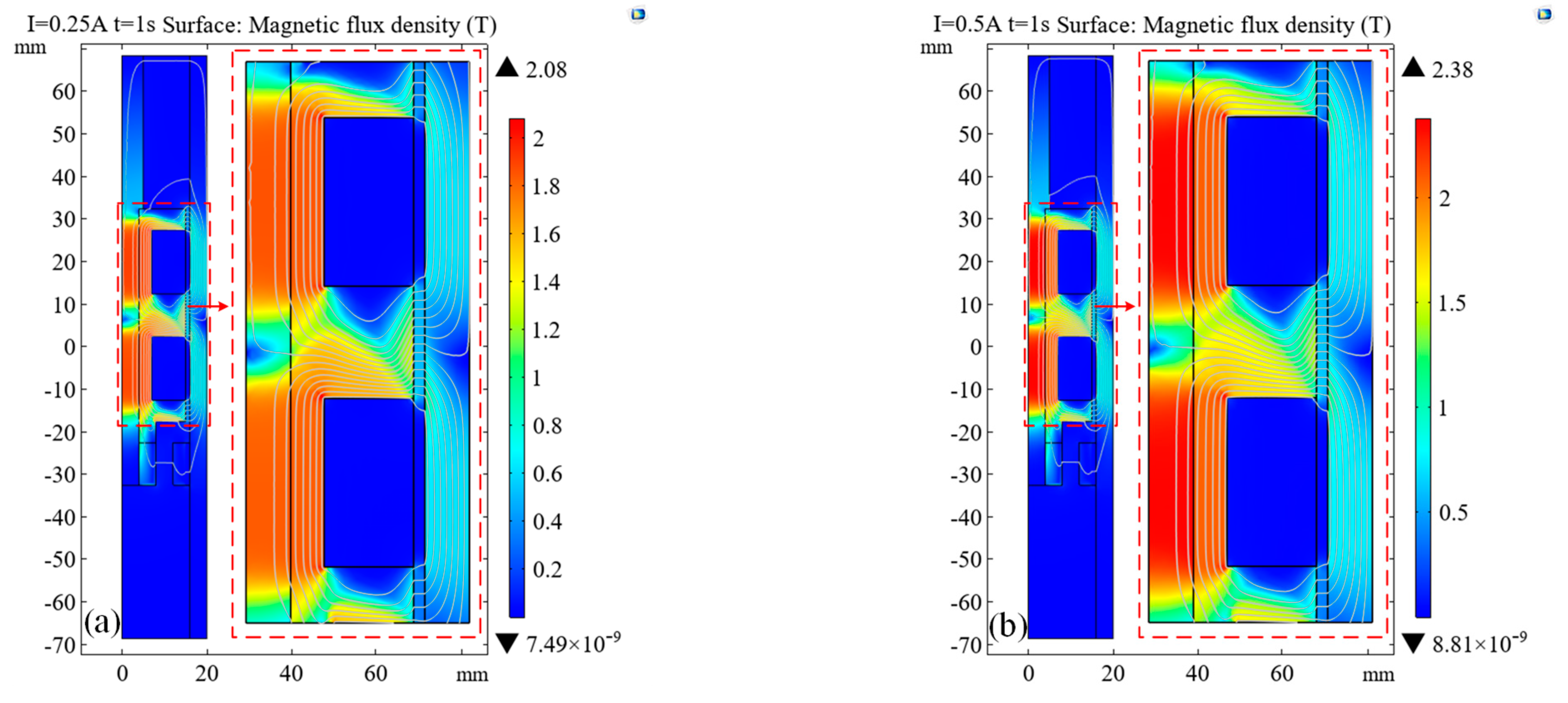
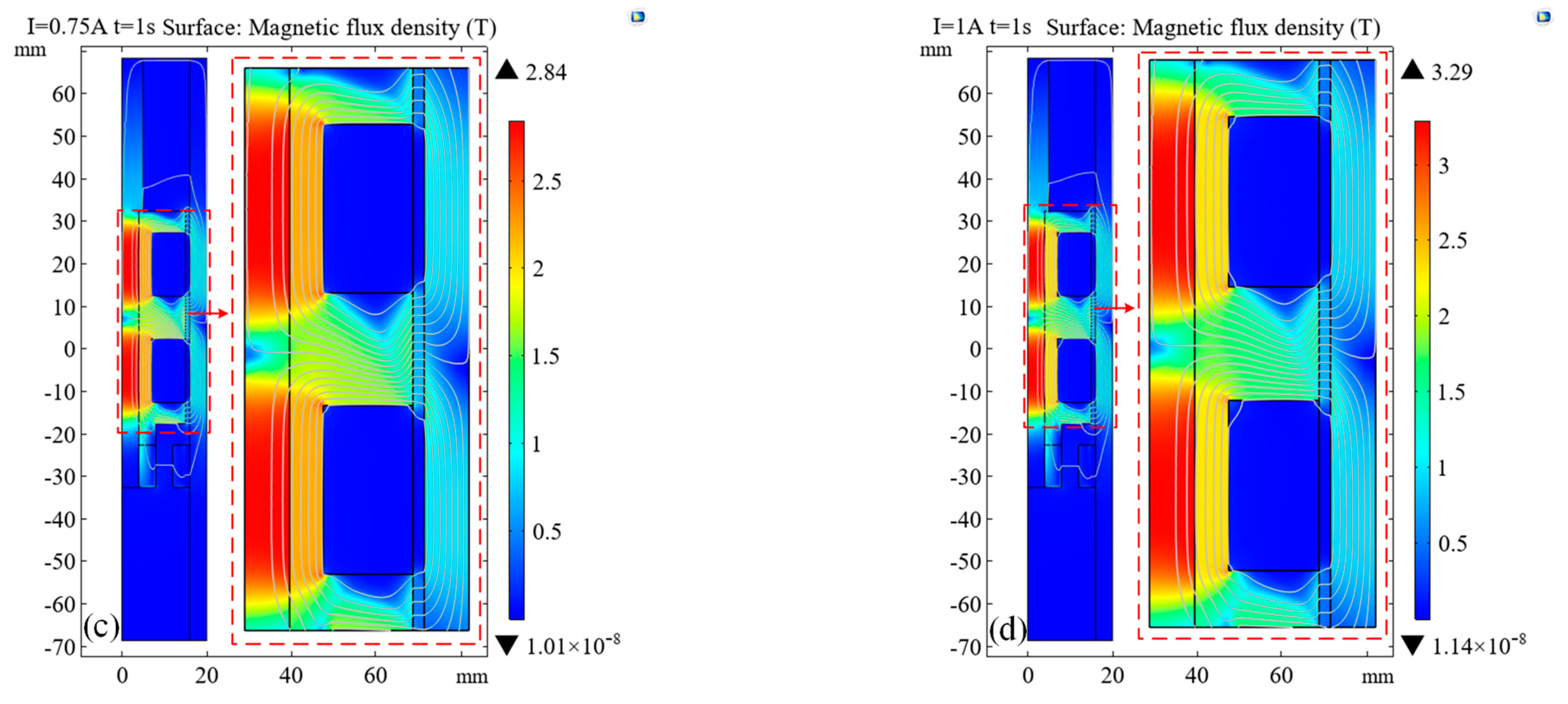
Figure 4.
Magnetic field distribution for: (a) I = 0.25 A; (b) I = 0.5 A; (c) I = 0.75 A; and (d) I = 1 A.
Figure 4.
Magnetic field distribution for: (a) I = 0.25 A; (b) I = 0.5 A; (c) I = 0.75 A; and (d) I = 1 A.
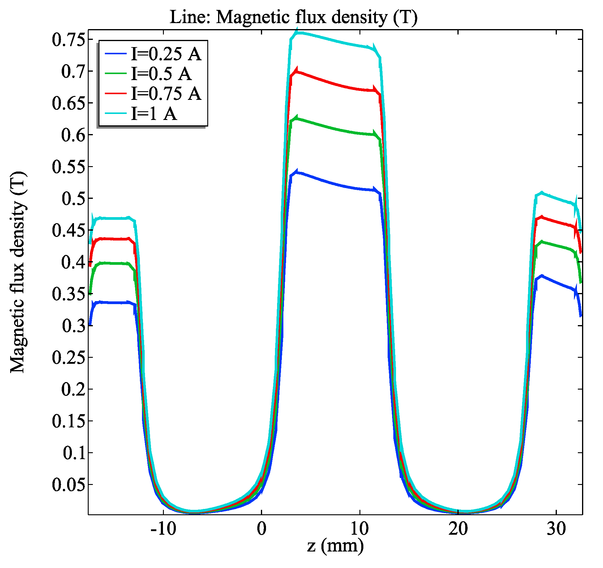
Figure 5.
Magnetic induction intensity in the middle line of damping gap at different currents.
Figure 5.
Magnetic induction intensity in the middle line of damping gap at different currents.
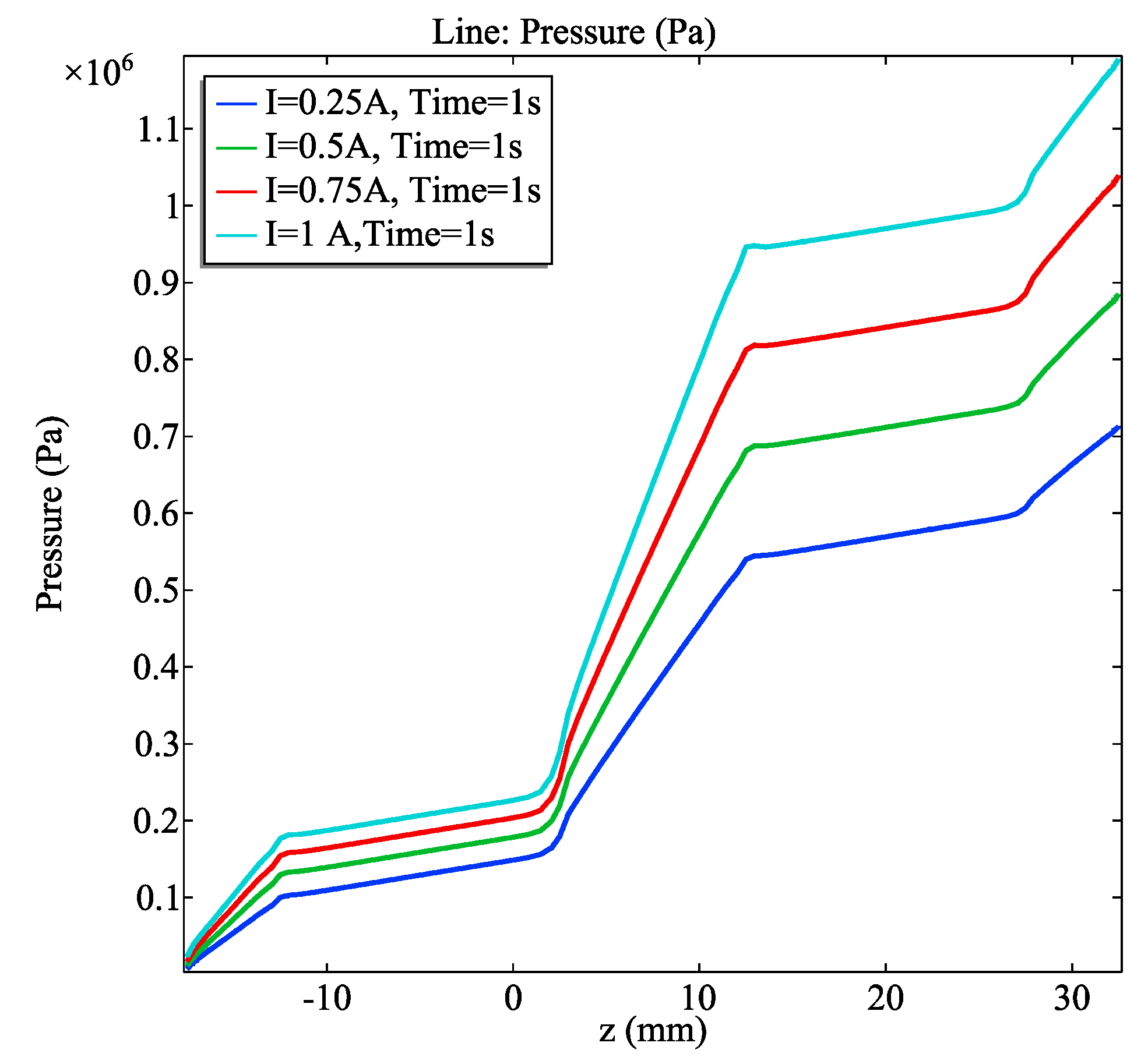
Figure 6.
The pressure of damping gap at different currents for I = 0.25, 0.5, 0.75, and 1 A.
Figure 6.
The pressure of damping gap at different currents for I = 0.25, 0.5, 0.75, and 1 A.
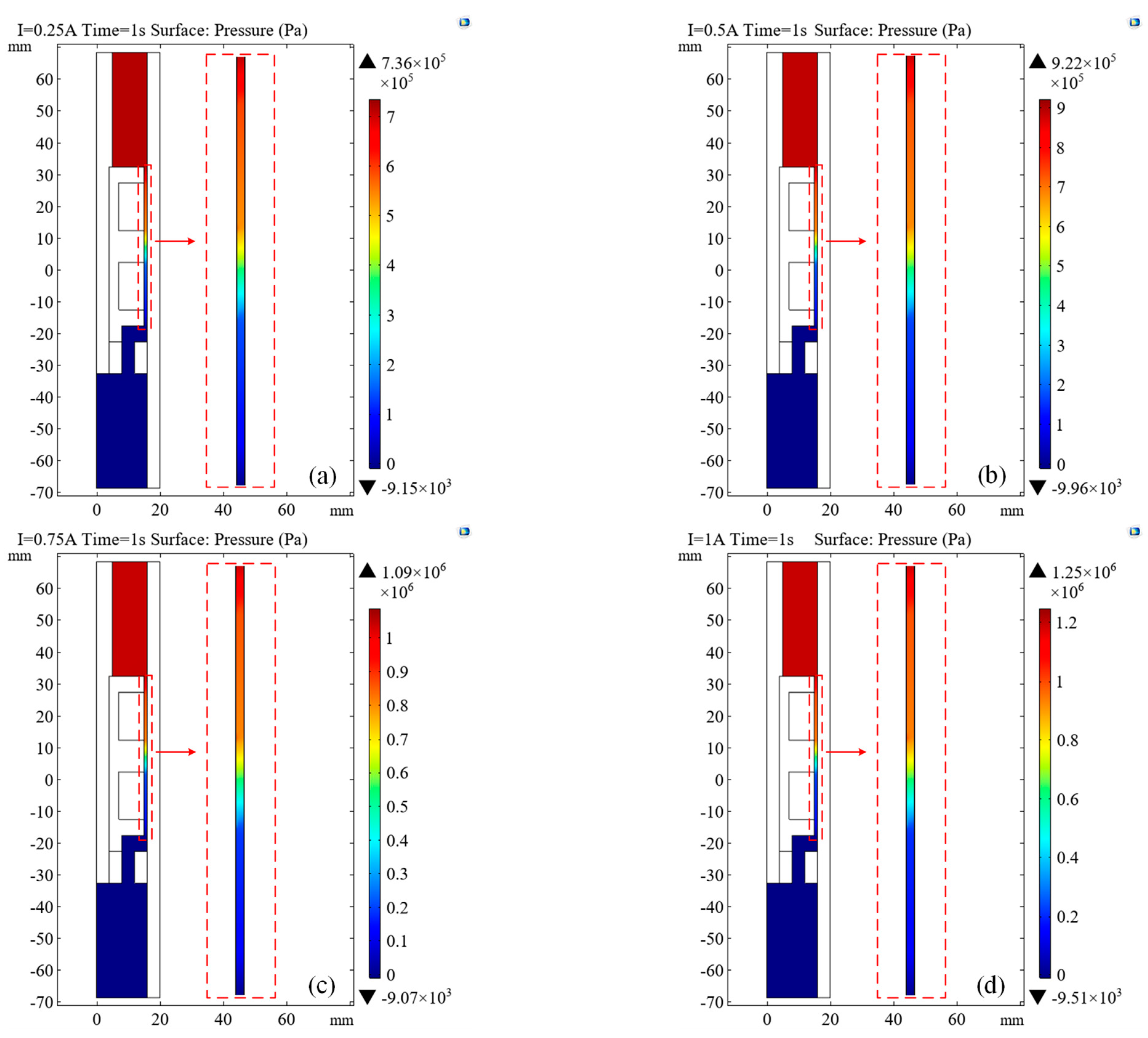
Figure 7.
Pressure distribution for: (a) I = 0.25 A; (b) I = 0.5 A; (c) I = 0.75 A; and (d) I = 1 A.
Figure 7.
Pressure distribution for: (a) I = 0.25 A; (b) I = 0.5 A; (c) I = 0.75 A; and (d) I = 1 A.
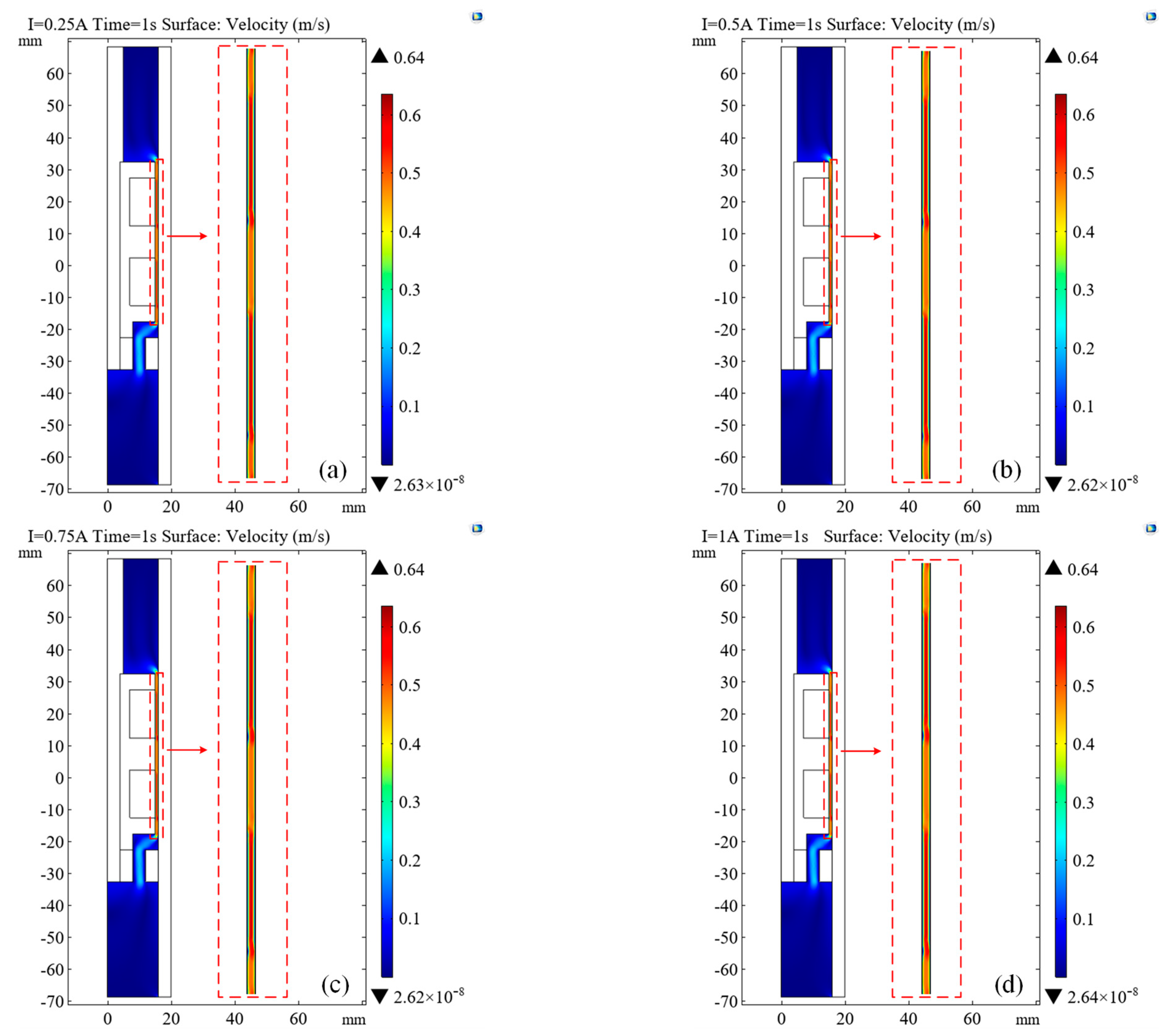
Figure 8.
Velocity distribution for: (a) I = 0.25 A; (b) I = 0.5 A; (c) I = 0.75 A; and (d) I = 1 A.
Figure 8.
Velocity distribution for: (a) I = 0.25 A; (b) I = 0.5 A; (c) I = 0.75 A; and (d) I = 1 A.
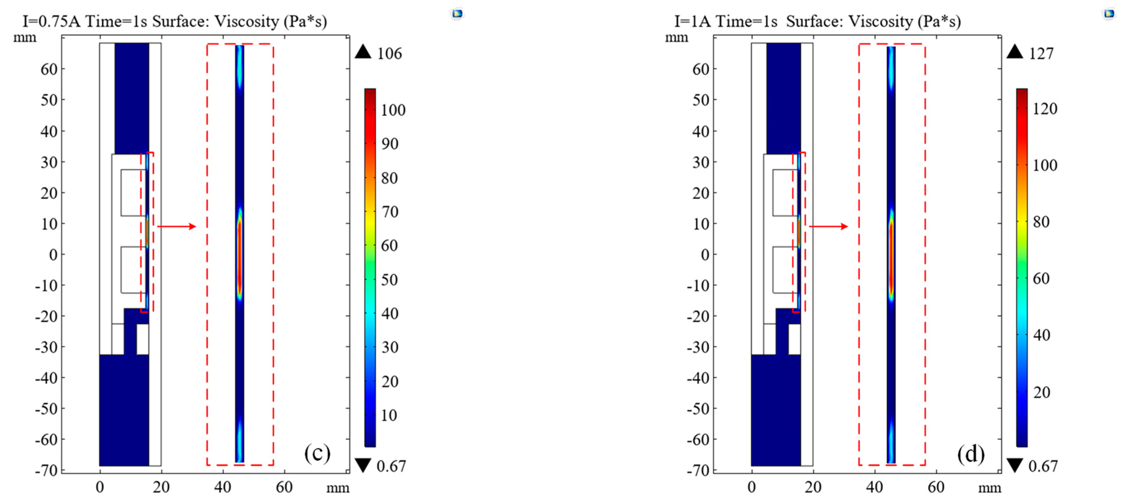
Figure 9.
Dynamic viscosity distribution for: (a) I = 0.25 A; (b) I = 0.5 A; (c) I = 0.75 A; and (d) I = 1 A.
Figure 9.
Dynamic viscosity distribution for: (a) I = 0.25 A; (b) I = 0.5 A; (c) I = 0.75 A; and (d) I = 1 A.
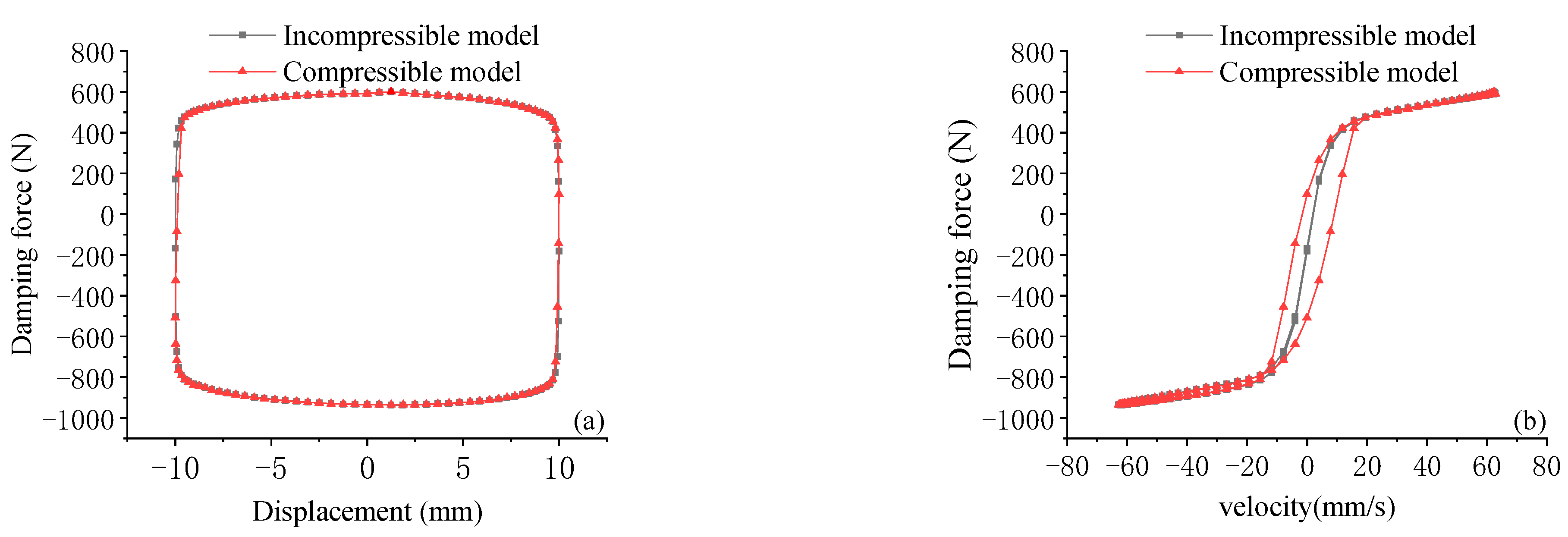
Figure 10.
Damping characteristic contrast considering compressibility and incompressibility: (a) damping force–displacement; and (b) damping force–velocity.
Figure 10.
Damping characteristic contrast considering compressibility and incompressibility: (a) damping force–displacement; and (b) damping force–velocity.
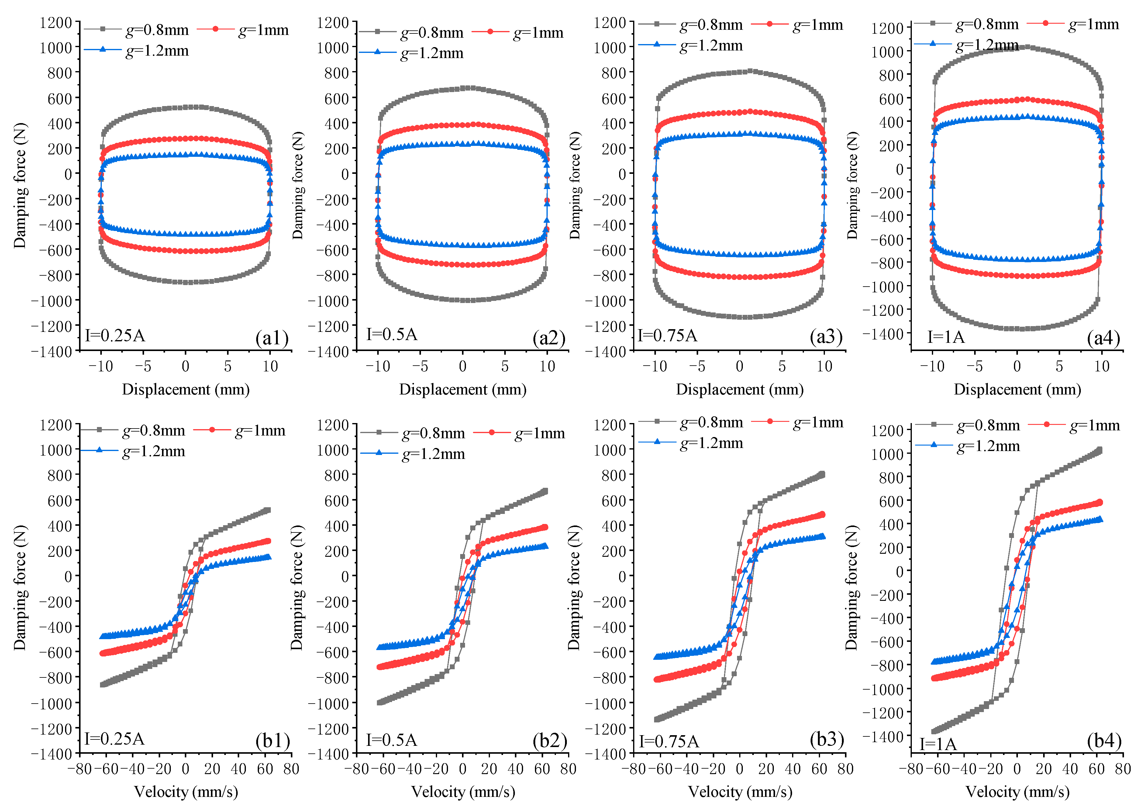
Figure 11.
Damping characteristics at different damping gaps for I = 0.25, 0.5, 0.75 and 1 A: (a1–a4) damping force–displacement; and (b1–b4) damping force–velocity.
Figure 11.
Damping characteristics at different damping gaps for I = 0.25, 0.5, 0.75 and 1 A: (a1–a4) damping force–displacement; and (b1–b4) damping force–velocity.
Figure 12.
Damping characteristics of effective magnetic poles at different ends for I = 0.25, 0.5, 0.75 and 1 A: (a1–a4) damping force–displacement; and (b1–b4) damping force–velocity.
Figure 12.
Damping characteristics of effective magnetic poles at different ends for I = 0.25, 0.5, 0.75 and 1 A: (a1–a4) damping force–displacement; and (b1–b4) damping force–velocity.
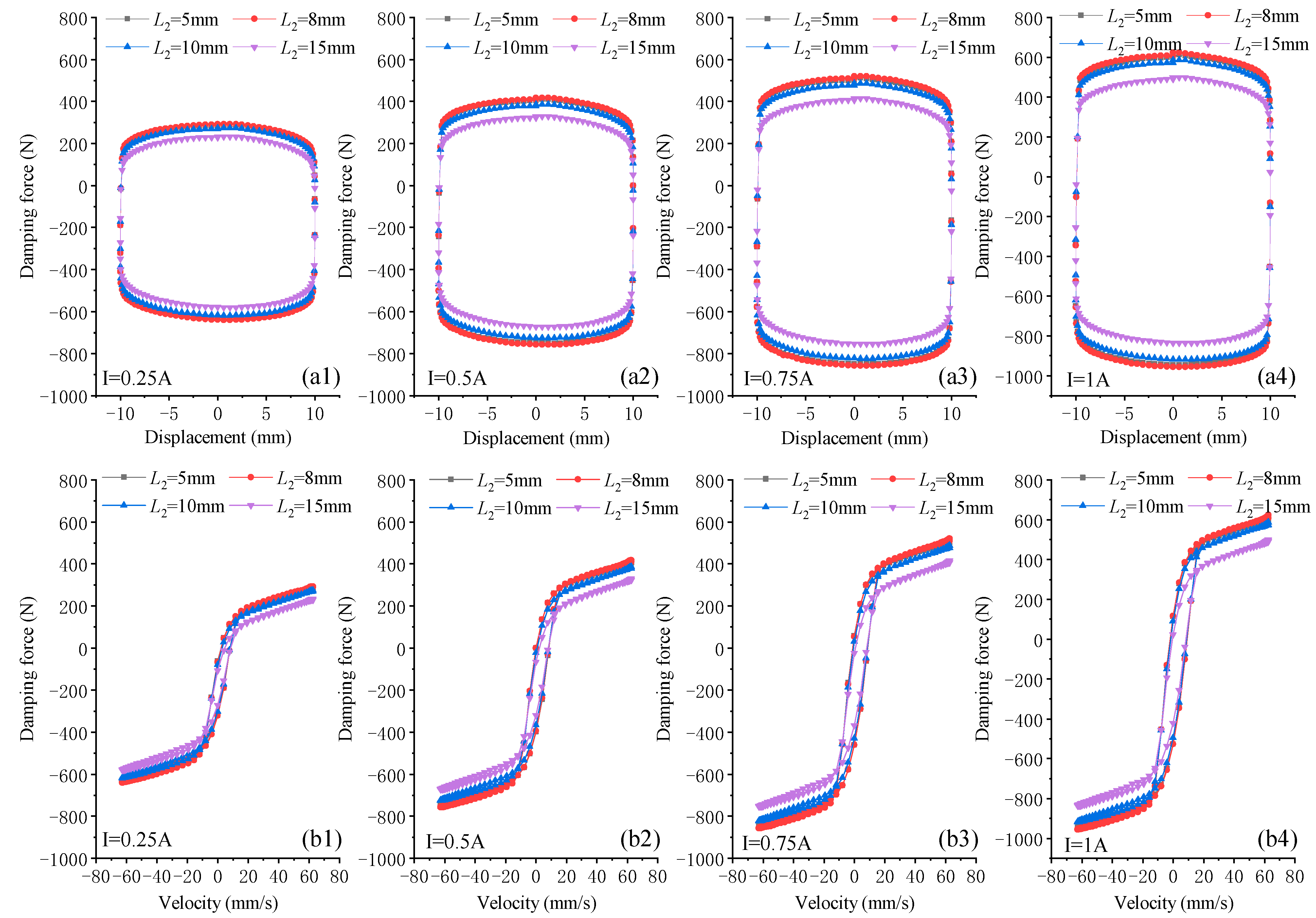
Figure 13.
Damping characteristics of effective magnetic poles in the middle for I = 0.25, 0.5, 0.75 and 1 A: (a1–a4) damping force–displacement; and (b1–b4) damping force–velocity.
Figure 13.
Damping characteristics of effective magnetic poles in the middle for I = 0.25, 0.5, 0.75 and 1 A: (a1–a4) damping force–displacement; and (b1–b4) damping force–velocity.
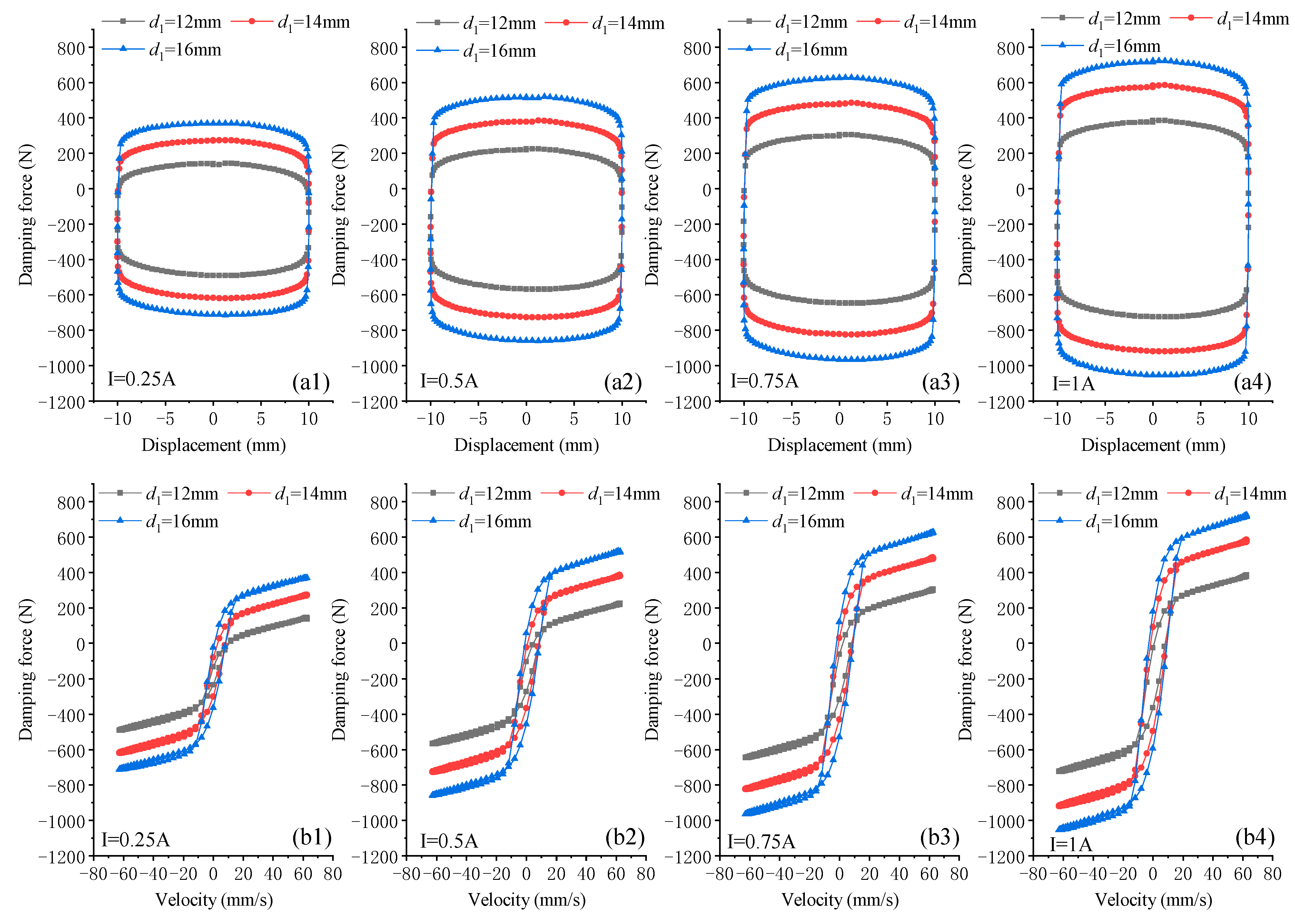
Figure 14.
Damping characteristics of different magnetic yoke diameters for I = 0.25, 0.5, 0.75 and 1 A: (a1–a4) damping force–displacement; and (b1–b4) damping force–velocity.
Figure 14.
Damping characteristics of different magnetic yoke diameters for I = 0.25, 0.5, 0.75 and 1 A: (a1–a4) damping force–displacement; and (b1–b4) damping force–velocity.
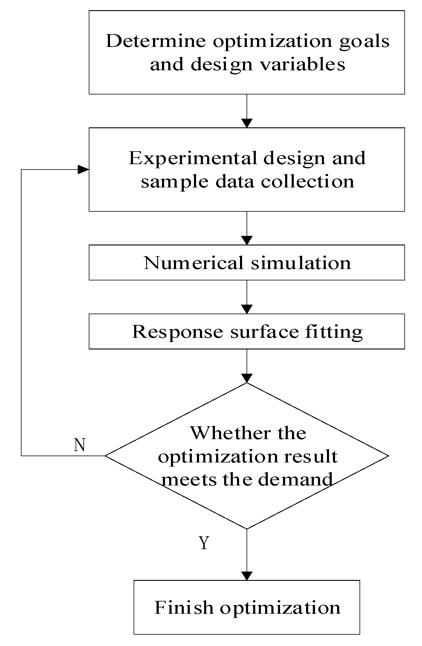
Figure 15.
Optimization process.
Figure 15.
Optimization process.
Figure 16.
Relationship between damping force and design variables: (a) damping force vs. A and B; and (b) damping force vs. C and D.
Figure 16.
Relationship between damping force and design variables: (a) damping force vs. A and B; and (b) damping force vs. C and D.
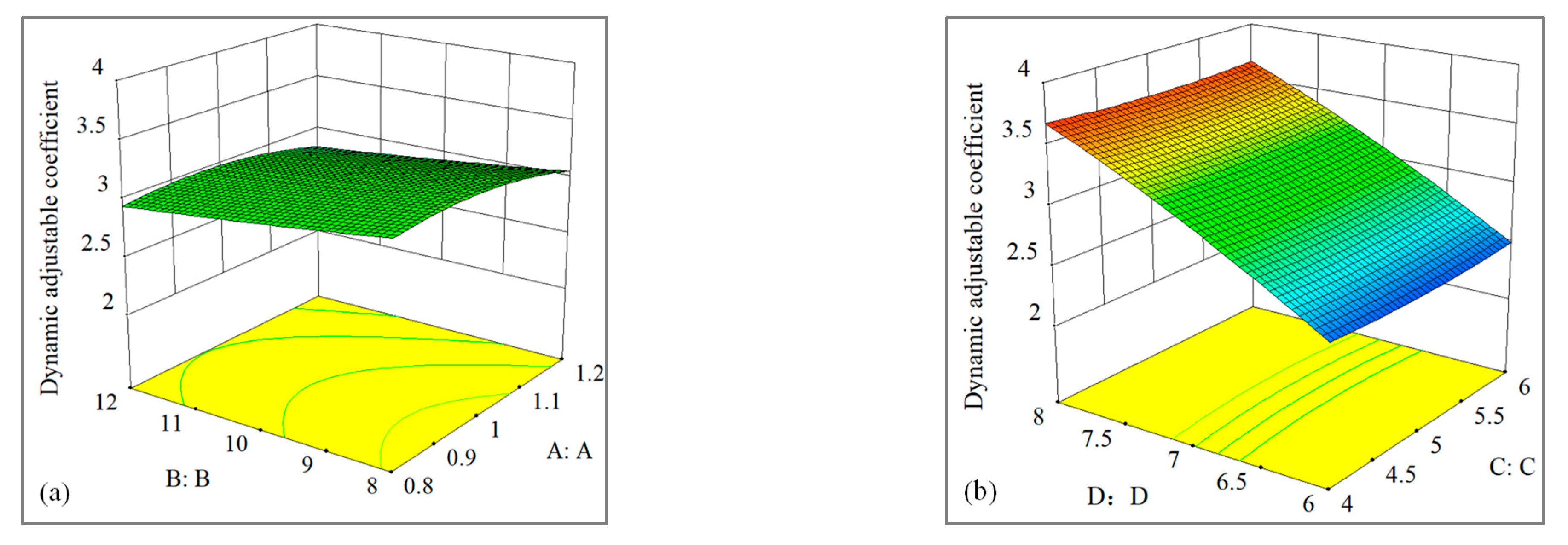
Figure 17.
Relationship between adjustable damping coefficient and design variables: (a) adjustable damping coefficient vs. A and B; and (b) adjustable damping coefficient vs. C and D.
Figure 17.
Relationship between adjustable damping coefficient and design variables: (a) adjustable damping coefficient vs. A and B; and (b) adjustable damping coefficient vs. C and D.
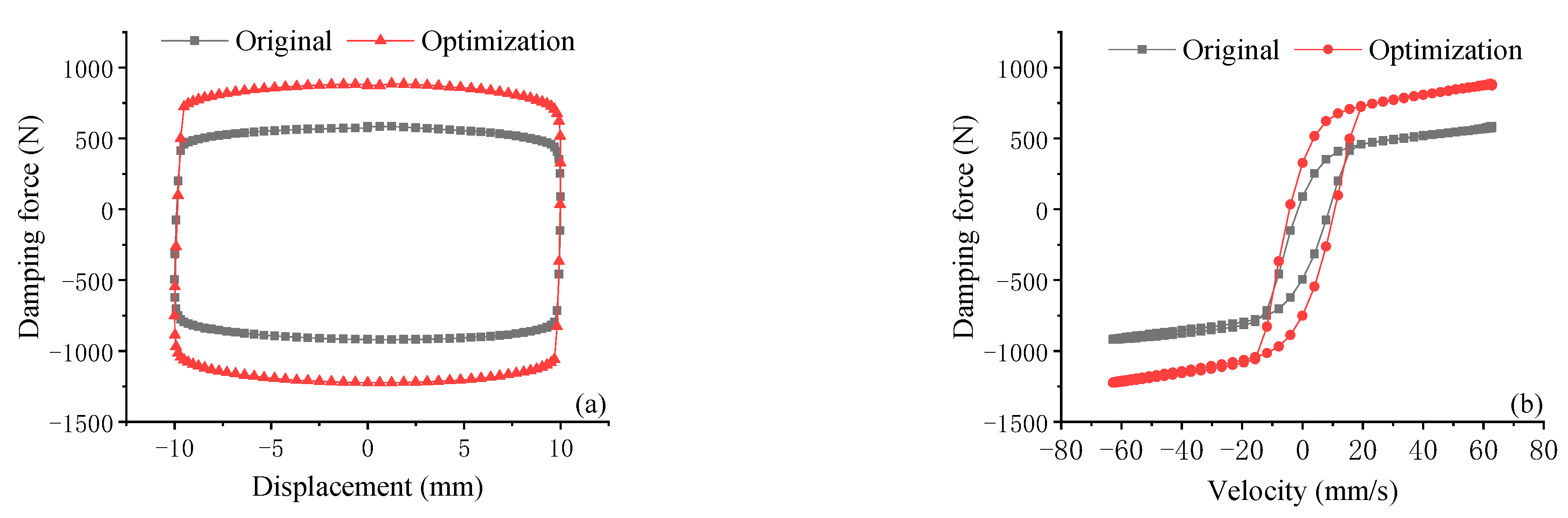
Figure 18.
Damping characteristics before and after optimization: (a) damping force–displacement; and (b) damping force–velocity.
Figure 18.
Damping characteristics before and after optimization: (a) damping force–displacement; and (b) damping force–velocity.
Table 1.
MR fluid properties.
Table 1.
MR fluid properties.
| Model Number | Properties | Value |
|---|
| MRF450 | density | 3550 (kg/m3) |
| viscosity (40 °C) | 0.69 (pa·s) |
| magnetizing curve | Figure 2b |
| shear stress vs. magnetic induction intensity | Figure 2c |
Table 2.
Main design parameters and initial values of the MRD.
Table 2.
Main design parameters and initial values of the MRD.
| Main Structural Parameters | Values |
|---|
| the thickness of the cylinder | 4 mm |
| piston rod diameter | 10 mm |
| piston diameter | 30 mm |
| yoke diameter | 14 mm |
| damping gap | 1 mm |
| magnetic pole length at both ends | 5 mm |
| magnetic pole length in the middle | 10 mm |
| loop length | 15 mm |
| current | 0.25 A, 0.5 A, 0.75 A, 1 A |
| number of turns per coil | 600 |
| compensation chamber pressure | 2.23 MPa |
Table 3.
Upper and lower limits of design variables of damper structure parameters.
Table 3.
Upper and lower limits of design variables of damper structure parameters.
| Code | Design Variable | Lower Limit | Middle | Upper Limit |
|---|
| A | damping gap | 0.8 | 1 | 1.2 |
| B | magnetic pole length in the middle | 8 | 10 | 12 |
| C | magnetic pole length at both ends | 4 | 5 | 6 |
| D | yoke diameter | 6 | 7 | 8 |
Table 4.
Design and results of response surface test.
Table 4.
Design and results of response surface test.
| Test Number | A (mm) | B (mm) | C (mm) | D (mm) | Fd(N) | |
|---|
| 1 | 0.8 | 8 | 5 | 14 | 1320.24 | 3.24 |
| 2 | 1.2 | 8 | 5 | 14 | 755.96 | 3.09 |
| 3 | 0.8 | 12 | 5 | 14 | 1212.54 | 2.93 |
| 4 | 1.2 | 12 | 5 | 14 | 694.25 | 2.81 |
| 5 | 1 | 10 | 4 | 12 | 723.45 | 2.46 |
| 6 | 1 | 10 | 6 | 12 | 721.09 | 2.42 |
| 7 | 1 | 10 | 4 | 16 | 1097.36 | 3.76 |
| 8 | 1 | 10 | 6 | 16 | 1097.07 | 3.71 |
| 9 | 0.8 | 10 | 5 | 12 | 1003.72 | 2.44 |
| 10 | 1.2 | 10 | 5 | 16 | 573.87 | 2.33 |
| 11 | 0.8 | 10 | 5 | 16 | 1457.94 | 3.55 |
| 12 | 1.2 | 10 | 5 | 16 | 827.86 | 3.37 |
| 13 | 1 | 8 | 4 | 14 | 953.38 | 3.3 |
| 14 | 1 | 12 | 4 | 14 | 875.49 | 2.96 |
| 15 | 1 | 8 | 6 | 14 | 967.97 | 3.27 |
| 16 | 1 | 12 | 6 | 14 | 886.74 | 3.01 |
| 17 | 0.8 | 10 | 4 | 14 | 1286.14 | 3.14 |
| 18 | 1.2 | 10 | 4 | 14 | 737.50 | 2.97 |
| 19 | 0.8 | 10 | 6 | 14 | 1281.74 | 3.11 |
| 20 | 1.2 | 10 | 6 | 14 | 734.41 | 2.99 |
| 21 | 1 | 8 | 5 | 12 | 766.36 | 2.59 |
| 22 | 1 | 12 | 5 | 12 | 705.98 | 2.39 |
| 23 | 1 | 8 | 5 | 16 | 1102.67 | 3.72 |
| 24 | 1 | 12 | 5 | 16 | 1136.07 | 3.61 |
| 25 | 1 | 10 | 5 | 14 | 918.05 | 3.10 |
Table 5.
Mathematical model of response surface.
Table 5.
Mathematical model of response surface.
| Response | Response Function |
|---|
| damping force | |
| dynamically adjustable coefficient | |
Table 6.
Variance analysis.
Table 6.
Variance analysis.
| Information | Standard | Fd | |
|---|
| Sum of squares | - | 1.34 × 10⁶ | 4.5 |
| Mean of aquare | - | 95,945 | 0.54 |
| F-Value | - | 145.57 | 68.01 |
| p-value | <0.05 | <0.0001 | <0.0001 |
| R2 | >0.9 | 0.98 | 0.98 |
Table 7.
Comparison of parameter values between the initial model and the optimized model.
Table 7.
Comparison of parameter values between the initial model and the optimized model.
| Parameters | A (mm) | B (mm) | C (mm) | D (mm) | Fd (N) | |
|---|
| before optimization | 1 | 10 | 5 | 14 | 918.58 | 3.10 |
| after optimization | 0.9 | 5 | 4 | 16 | 1222.34 | 3.63 |

 ,
, 


