Abstract
This article presents an innovative legged-wheeled system, designed to be applied in a hybrid robotic vehicle’s locomotion system, as its driving member. The proposed system will be capable to combine the advantages of legged and wheeled locomotion systems, having 3DOF connected through a combination of both rigid and non-rigid joints. This configuration provides the vehicle the ability to absorb impacts and selected external disturbances. A state space approach was adopted to control the joints, increasing the system’s stability and adaptability. Throughout this article, the entire design process of this robotic system will be presented, as well as its modeling and control. The proposed system’s design is biologically inspired, having as reference the human leg, resulting in the development of a prototype. The results of the testing process with the proposed prototype are also presented. This system was designed to be modular, low-cost, and to increase the autonomy of typical autonomous legged-wheeled locomotion systems.
1. Introduction
Autonomous robotic systems are increasingly present in our daily lives. From robotic vacuum cleaners for domestic use, to cargo transportation systems in industrial environments, there is a growing demand for automated and robotized systems. These are projected to have the ability to assist humans in their daily life, and even, to provide new possibilities, that until now would not have been possible.
One of the current trends is the growing use of mobile robots to perform tasks in different locations. The proof of this can be found in publications related to the development of autonomous robotic vehicles and in thousands of patents filed since 2010.
Hybrid locomotion systems are also an increasing trend, since these robotic systems exploit the advantages of using more than one locomotion system simultaneously. Their subsystem—the legs—makes their mobility unique, increasing their ability to move through difficult terrain, as well as increasing their stability, based on the multiple Degrees of Freedom (DOFs) use. Innovative and successful examples of vehicles of this type are described in this section.
The robot Momaro [1], developed by the University of Bonn, combines four legs and two wheels, and its base footprint has a size of 800 × 700 mm (L × W); its height was not mentioned. The authors used commercial off-the-shelf components, namely Robotis Dynamixel actuators. Each leg has 4DOFs, and each wheel adds 2DOFs to the configuration. It weighs 58 kg and its power supply is 22.2 V. Publication [1] did not mention the speeds reached, nor the payload, but a series of actions that the robot performed during a 2017 challenge.
CENTAURO [2] is a hybrid vehicle, developed at the Instituto Italiano di Tecnologia, with four legs and two arms measuring 610 × 615 × 1706 mm (L × W × H). The authors developed their own actuators to achieve a modular design, with a high power/strength density. The motion range of the legs was designed for the robot to operate in different formations, including inward and outward arrangements. Each leg has 5DOFs, combining spider-like and mammalian leg configurations. The robot weighs 92 kg and works at 48 V. In [2] two studies were presented, one achieving 0.1 m/s walking speed and another 1.6 m/s by moving on wheels, with a payload of 60 kg.
The team of the Robotic Systems Lab at ETH Zurich developed ANYmal [3], and the improved ANYmal on wheels [4], which is a quadrupedal robot, 0.5 m tall and weighing 30 kg. The ANYmal’s configuration involves 3DOF legs, being adapted to accommodate wheeled locomotion, achieving a speed of 2 m/s with hybrid locomotion, consuming 156 W.
Although not exactly in the same category, there are some other legged-wheeled locomotion projects, such as the robots ASGUARD [5], WR-3 [6], EHR [7], Quattroped [8], WheelTransformer [9], TH-Weng [10], and the work presented by Qiao et al. [11].
Another similar research topic involves the development of platforms for lower limb rehabilitation [12]. The work of Hu et al. [13] is another successful example of the use of a 3DOF solution for rehabilitation and impedance control. The work of Wu et al. [14] is another example of a 3DOF lower limb rehabilitation robot, with a structure similar to that used in the case of the solution presented in this article and that serves this purpose. Feng et al. [15] also proposed a similar solution, using static torque sensors.
Throughout this article, the design of an individual leg for the Legged-Wheeled system to achieve Hybrid locomotion is introduced, as well as the models and proposed controllers. Each leg uses a strategic combination of rigid and non-rigid joints, as well as a driving wheel and a support wheel. The latter enables a low-power mode and increases stability on regular terrain. A non-rigid joint increases the compliance of the leg, as well as its ability to deal with uneven terrain and unexpected disturbances.
Typical legged-wheeled systems have a great power consumption, since its joints need to be constantly moving, in order to maintain the position and stabilize the vehicle. On the other hand, these vehicles tend to be very expensive and highly customized for specific applications, being very difficult to modify. The presented work differs from these by being a low-cost solution and completely modular. It also differs from some brushless DC motor driving solutions, because the use of brushed DC motors with gearbox decreases the power consumption, thus increasing the robot autonomy, although providing less torque to the joint. In addition to this, a low-power configuration is also introduced, in order to further reduce the energy consumption.
Even though the built prototype can be controlled in the y axis, in addition to the wheel speed, in this paper the focus is on the state-space controllers of both the rigid and non-rigid joints. This option was taken because the control of the hip joint and the lower wheel is implemented using more traditional solutions, namely PID controllers.
The paper is structured as follows. After the introduction in Section 1, which presents the state-of-the-art, Section 2 presents the design and mechanical model of the developed leg, as well as its mathematical model and the kinematics of the members. Throughout Section 3, the developed tests are presented, as well as the obtained results. Finally, Section 4 presents the conclusions and future work.
2. Design, Modeling, and Control
The proposed system was designed to be applied on a platform based on a mobile hybrid locomotion system (provided later in Section 4). For this system to be suitable from a research point of view, it needed to be focused on three principles:
- Low-cost—The system must be affordable so that any changes that need to be made do not have a significant impact on the vehicle’s prototyping and maintenance budget.
- Expandable—The vehicle must be able to be expanded and thus it must be designed to have easy adaptability to allow, for example, the incorporation of new sensors, actuators, and tests with different systems and algorithms without much mechanical effort;
- Modular—The system must be easily changed only in one of its parts, which implies that its design has to be modular, in order to be able to be changed locally, not having the need to completely change the robot, thus this task is very time consuming.
In addition to these principles, it is also important to mention, as previously, that it is adequate for a hybrid vehicle to operate in environments with different characteristics. In this specific case, the vehicle should also be able to deal with nonstructured environments, as it is the closest to reality. So, taking these premises into account, the design of the locomotion system was developed, being presented below.
2.1. Mechanical Design
Regarding the mechanical part, it was necessary to make a set of decisions to allow the correct design right away. So, it was considered that the purpose of this solution for indoor, as well as outdoor navigation, is that it should be a low-cost and modular solution. In addition, it was taken into account that the proposed solution should use brushed DC motors and that the vehicles in which this system can be applied are aimed to be used in nonstructured environments. Thus, the following decisions were made:
- The system must be transportable in a regular car trunk, both in size and weight;
- The system will be included in a robot with four limbs, which must follow a legged-wheeled configuration, with the wheel at the end of the leg;
- The robot in which the legs will be used must be able to navigate in three modes: purely legged, purely wheeled, and hybrid;
- As a vehicle with energy consumption above the average for a mobile robot, it should incorporate a low-power configuration in which energy consumption is reduced to the minimum possible, being a particular case of the purely wheeled mode;
- Given the components’ size and the scale of the motors, it was decided that the legs would have approximately 1:3 on a human scale;
- Each one of the limbs and their integrated parts must be easily assembled and disassembled;
- The uppermost joint should be able to allow each limb to rotate from − 90° to 90°, allowing linear movement in x and y, rotation around the vehicle’s own axis, as well as steering the vehicle in purely wheeled navigation;
- To achieve the previous assumptions, each limb must have 3DOF, two of which are located on an upper point, considered one of the rotation axes of the hip and a second just below, which adds another axis of rotation in a perpendicular direction. Finally, a third DOF is added, considered the knee. In place of the foot there will be a wheel, which will be motorized;
- To be able to accommodate impacts, floor irregularities, and better deal with obstacles, one of the joints in each limb must be non-rigid;
- The limb configuration must be able to sensor force, allowing compliance in movements and attitudes;
Considering the desired scale for the dimensions of the leg-wheel, as well as an average human height of 1700 mm, it was decided that the total length should be around 550 mm, and therefore, each link should have about 275 mm.
Then, for the limbs design, taking into account the requirements of low cost, easy expansibility, and modularity, it was decided to use 3D printing as the main source of development of the mechanical parts. In addition, it was decided to use the material Polylactic Acid (PLA) for its quality-cost ratio. This solution greatly reduces the cost of obtaining parts for the vehicle, both economically and also temporally, since the material cost is considerably lower as well as the speed of 3D printing is considerably higher compared to, for example, CNC (Computer Numerical Control) machining.
Regarding the decision making, of which joints should be non-rigid, it was decided to define the one closer to the hip joint, as it increases the number of situations in which its properties can be useful. In a case of an obstacle surpassing like the one shown in Figure 1, it is understandable that the joint that moves the most and is capable of accommodating this irregularity is the top joint, since the lower joint z movement capability is reduced. As mentioned in the figure, it is noticeable that this configuration is capable of handling horizontal and vertical impacts, as well as floor irregularities. The only configuration where this joint does not exhibit its vertical absorption capability is when it is fully stretched. This non-rigid joint is the one described in a previously published work [16]. The rigid joint follows the same circular configuration and size; however, it connects directly to the motor shaft. Taking into account the modularity requisite, the half-link where the joint is screwed is the same for both joints, just changing the joint itself.
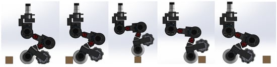
Figure 1.
Obstacle surpassing simulation.
Regarding the support parts and alignment of the joints, it was decided to use the internal bearing of the motor and its shaft to support one side and to use another bearing to support and reduce friction on the other side of the joint. Having considered that, a rotating shaft with a larger diameter adds strength and slightly reduces the possibility of clearances, it was decided to use a bearing with a 20 mm internal diameter (6004 2Z). For the alignment and support of the wheel, the same concept was used, differentiated by the use of a smaller (12 mm) diameter bearing (6001 2Z).
Since it is necessary to accurately sense the forces exerted on each leg link, it was decided to divide it in half and use a load cell to couple both. With this configuration, there are two complementary measures of the force exerted on the leg.
To fulfill the requirement of having a low-power configuration, in which the vehicle can navigate with a substantially reduction of its energy consumption, it was decided to design the last link with an inclination, as well as to use an omnidirectional wheel, allowing the leg to rest on the ground, eliminating the consumption of two motors, leaving only the wheel rotation motor and the leg steering motor. In addition, for this purpose, an omnidirectional wheel was added, allowing greater stability of the platform. In this traction configuration, the platform will have four driving wheels and will use four free support wheels on the ground. Although they have a fixed axle, when using omni wheels, it allows the vehicle, by rotating its legs, to also have omnidirectionality.
At the bottom of each leg, it was decided to use rubber wheels with a 100 mm diameter, since smaller wheels reduce the angle of action of the leg. This is explained since the wheel support easily started to hit the floor when the leg is rotated, although with a low angle.
One of the purposes of the applied leg configuration is that it can rotate at least 180° (90° for each side), thus allowing lateral movement. In addition, it was thought that for simpler kinematics, the wheel’s support point should be aligned with the rotation axis of the hip joint. That said, it was decided that the hip joint would use a C structure that would cover both specifications. The final solution, with the respective joint numbering and rotation axis is presented in Figure 2.
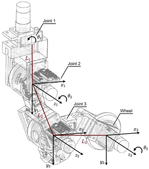
Figure 2.
Leg with axis, links, and joints numbering.
2.2. Electrical Design
Regarding the electrical design, there are some considerations to take into account. First of all is the type of motor to be applied. Considering that it is an objective to use the vehicle in autonomous mode, as well as the use of Series Elastic Actuators (SEA), it was decided to use DC motors with a gearbox. After some tests that were carried out and presented in previous publications (Ref. [17], preceded by Ref. [16]), it was found to be more convenient to use in-line gearboxes. The used motors were those from CQRobot, being decided to use different gearboxes. Namely, the motor used for joint 1 is the CQR37D64CPR70GR, with a gearbox ratio of 70:1 and top speed of 157 RPM, joints 2 and 3 have the same type of motor—CQRGL20180525-52GB—with ratio of 210:1 and top speed of 52 RPM, and finally for the wheel the used motor—CQR37D64CPR43.8GR—has a 43.8:1 gearbox with maximum speed of 251 RPM. Each motor uses its own driver—BTS7960—enabling the control of motors up to 30 V and 43 A. To transmit each joint angular position, each motor has an built-in incremental encoder, from which the relevant information for the motor control is collected. In addition to this, and taking into account that there are non-rigid joints, it was considered important to use an absolute encoder for each of the three upper joints (1, 2, and 3). For this purpose, a high resolution (14-bit) rotational position sensor—AMS AS5048A—was used, which communicates through the SPI (Serial Peripheral Interface) protocol to transmit the readings.
Connecting each of the L2 and L3 semilinks, two load cells—TAL220—of 10 kg are mounted, thus allowing to measure the strength that each of the links is sensing in real time, using this information to apply the closed-loop control. In order to increase its sensitivity, an Amplifier—SEN 13879—is used for each cell, which uses the HX711 integrated circuit.
To receive data from the sensors that each leg has, as well as to control the drivers associated with each motor, two Arduino Nano 33 IOT were used. In addition to being a small solution, at a relatively low cost, these microprocessors have an embedded IMU that can be used to know the joints orientation, in which they are mounted. To facilitate the connections to the respective peripherals, an I/O Shield was used in each Arduino, after which a large part of the connections were made through Jumper Wires.
In order to facilitate connections, but also because the number of I/O ports easily starts to be large due to the use of a high number of sensors, each leg is “divided” into two. The set of the two motors of Joint 3 and Wheel, its relative encoders, the absolute encoder of Joint 3 and the load cell of the L3 link are connected to the Arduino that is in the adapter of Joint 3, while the other motors and sensors are connected to the Arduino that is in Joint 2.
Finally, in order to synchronize both Arduinos, since the implementation of the inverse kinematics for the leg movement requires that the commands are sent for all the joints at the same time, serial port 1 (set on RX/TX pins) is used. For this, a connection between the two pins from each Arduino is performed.
The connections diagram for each leg is shown in Figure 3, while Figure 4 presents the electric diagram including all the physical connections between the hardware.
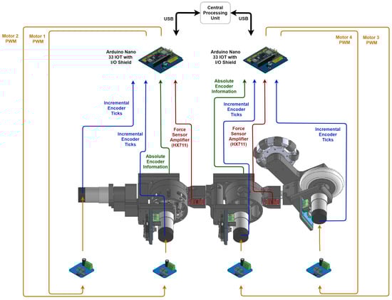
Figure 3.
Leg connections diagram.
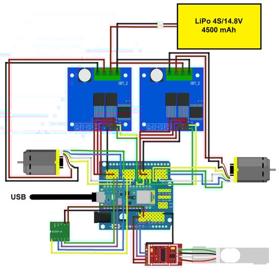
Figure 4.
Half-leg electric schematic connections.
After presenting all the theoretical characteristics of the mechanical design of the leg, Figure 5 presents the prototype built for testing. It is also presented in Table 1, including the components used to build this prototype, as well as their price range.
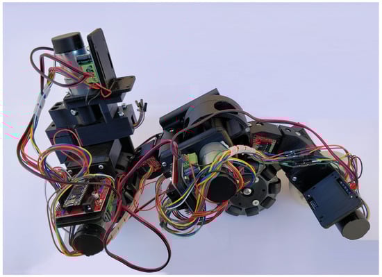
Figure 5.
Developed leg prototype example.

Table 1.
Components and price range for the prototype construction.
2.3. Modeling and Control
Considering that changing the configuration of just one joint to a complete leg changes the model presented in [16], it was necessary to expand the conceptual representation of each joint. Using these, it becomes possible to obtain the system of equations that follows. The motor model that was used for both models and conceptual representations was the one presented in Equation (1), that was then rearranged to the one presented in Equation (2) to be used further ahead. In these, u represents the system’s applied voltage (V), R the motor resistance (Ω), i the current that flows through it (A), k the motor constant (N·m/), and the angular speed (rad/s). The motor’s static friction torque (N·m) is given by the multiplication . It is important to state that the used motor model assumes that = while < , this way explaining the existence of the motor dead zone, which is a nonlinear element of the model. However, despite this, it can be neglected, given that it was proven in [16] that it is almost nonexistent and otherwise it will turn the defined system into a nonlinear one.
For control purposes, along the article, the first joint will be disregarded, being the controllers developed only for trajectories across the plane. This option is justified with the fact that the first joint will only be actuated with the other joints stopped so it will not be interesting to explore this DOF.
2.3.1. Non-Rigid Joint
Regarding the non-rigid joint, the respective conceptual representation is presented in Figure 6. Then, using it, one can obtain each joint model, presented in Equations (3) and (4), where are the moment of inertia (kg·m2), the motor torque (N·m), the respective angular speeds (rad/s), the viscous friction coefficients (N·m·s), the angular positions (rad), the springs constant (N/m), the damping coefficient (N·s/m), d the distance (m) between the joint and a mass m (kg) and finally g the gravity constant (m/s2).
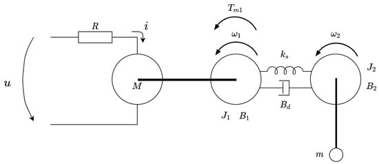
Figure 6.
Non-Rigid joint conceptual representation.
Now, using the rearranged Equation (2), it is possible to obtain the following equations, rearranged as well.
Using Equations (7) and (8) and transforming them into a state-space model in the form of Equation (9), it becomes:
The function applied to find the system’s transfer function was the one presented in Equation (13), and the obtained transfer function is presented in Equation (23).
To obtain the joint’s model parameters, a test was carried out where a sinusoidal sweep joint was applied, i.e., a sinusoidal signal was applied with a constant amplitude but with a variable frequency and maximum time. This option was taken to make it possible to excite the system in various regimes, so that its model is as close as possible to the reality. The whole process is parameterized to allow an excitation of the system in multiple modes.
For the non-rigid joint data collection, a wave with an amplitude of 60% was applied, with a starting frequency of 0.1 Hz, final frequency of 2.5 Hz, and a total time of 20 s. The following Equation (21) presents the values obtained for the beta parameters introduced in Equations (17) and (18). It is noticeable that these parameters seem well estimated since, for example, the values of and are practically symmetrical.
This model originated the following result, which can be compared to the data obtained in the test through the graphic on Figure 7.
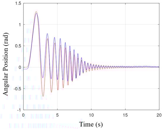
Figure 7.
Non-Rigid joint model vs. real angular positions.
Given this model, the obtained transfer function is presented below.
Another change from the solution proposed in [16] is the control. Bearing in mind the tuning limitations of the previously implemented controllers, which quickly became unstable, it was decided to use a state-space control technique. This technique is also better suited since the non-rigid joint has two different angular measurements, one from the relative and another from the absolute encoder. Thus, the state space controller uses both relative and absolute positions to calculate the plant controller’s output. Additionally, to reduce the noise from the sensor readings and to better the estimation of the variables that are not known directly, a state observer was implemented, thus improving the system’s performance. By applying the observer, the settling time was able to be decreased, as well as the trajectory and positioning errors reduced. For this joint, the considered reference signal is the absolute position and the block diagram for the implemented controller is presented in Figure 8 and it is further explored and explained.
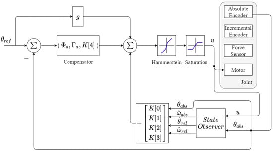
Figure 8.
State-space controller block diagram non-rigid joint.
The model presented above is a continuous time; however, the controller will be applied in a discrete system, so it is necessary to obtain the discrete time model. Using a Zero Order Hold (ZOH) equivalent to discretize the system, as proposed by Vaccaro [18], if the value of is known at some time :
where is the exponential matrix function and using and for the discretization, where T is considered the sampling period, the update equation becomes:
Since during the interval of integration the function is equal to , due to the ZOH being constant, Equation (25) becomes:
Thus, defining a discrete-time state vector and considering the new nomenclature , the discrete-time state-space equation becomes:
Using the Van Loan method to compute integrals involving the matrix exponential [19], a matrix M can be used to obtain the ones by computing the obtained matrix:
The designed controller is capable of following a step input, so it was decided that an additional dynamic will be introduced in the system to enable this feature. Another plus is that this additional dynamic also makes the system capable of dealing with disturbances of the same kind—unitary step disturbances. To add this to the state-space model, matrices must be defined as:
Now, a Bessel polynomial with a stabilizing time will be used, as presented in Equations (34)–(36).
Using the Ackermann’s formula [20], the controller constant vector can be found.
Finally, the calculated controller gains are obtained and introduced in the system. These gains are presented below in a matrix form.
As can be validated by the results presented in Figure 9, the controller provides very satisfactory results, reaching the reference value in about 1.5 s, a settling time of 0.9 s (considering 2% range), and an overshoot of approximately 1.5%.
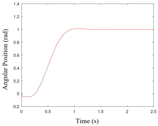
Figure 9.
Non-Rigid joint simulated controller.
2.3.2. Rigid Joint
Regarding the rigid joint, it was decided that it will be controlled using the relative encoder information, i.e., the relative angle and velocity. As previously mentioned, Equations (1) and (2) are still valid for this joint, since the physical motor and its model are the same; however, the proposed model is no longer the same as for the non-rigid joint. The new conceptual representation is shown in Figure 10 and originates the following equations.
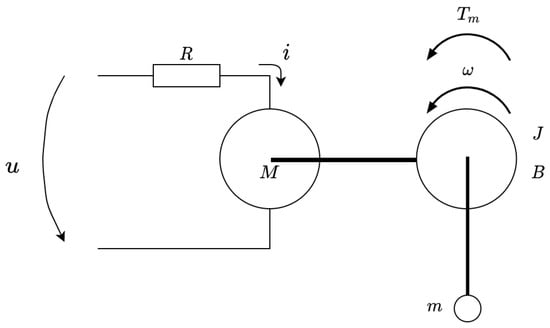
Figure 10.
Rigid joint conceptual representation.
The generic model for this joint is presented below, having considered the above equations to develop the matrix system.
For this joint a sinusoidal sweep was also used, with an amplitude of 40%, starting frequency of 0.2 Hz, final frequency of 5 Hz, and a total time of 10 s. The obtained parameters were the following.
Given this model, the obtained transfer function is then presented.
The additional dynamics matrices, as in the previous joint, are equal to 1 to implement the controller’s ability to deal with unit step disturbances.
The matrix containing the calculated controller gains is now presented.
The presented model originated the following result, which can be compared to the data obtained in the test through the graphic on Figure 11.
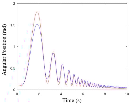
Figure 11.
Rigid joint model vs. real angular positions.
Although the rigid joint can have a more traditional control, using simpler controllers, it was decided to also use a state space approach. This is due to the fact that this joint, despite being rigid, may undergo more oscillations, due to its connection to the non-rigid joint but also to the fact that with this controller, the joint’s response is more comprehensive and is also able to deal with step disturbances. Unlike the non-rigid joint, the considered reference signal is the relative angular position, in order to reduce the noise from the absolute encoder, and the block diagram for the implemented controller is presented in Figure 12 and is further explored and explained.
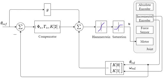
Figure 12.
State-space controller block diagram rigid joint.
As can be validated by the results in Figure 13, the simulation result, after the implementation of the described controller, reaches the reference value in about 0.7 s, a settling time of 0.5 s (considering 2% range) and without overshoot.
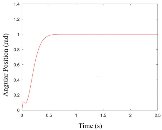
Figure 13.
Rigid joint simulated controller.
Knowing the data from the angular positions of a manipulator, the Denavit–Hartenberg method (DH) of direct kinematics can be used to obtain the values of the x and z points from the tip. Since the developed leg can be compared to an anthropomorphic manipulator, this method will be used to discover the coordinates of the wheel with respect to the measured angles. Considering the constants presented in Figure 2, Table 2 has the DH parameters for the developed leg.
Table 2.
DH parameters for the leg.
Considering the lengths measured and presented in Table 3, the coordinate transformation matrix obtained through the DH method is shown in Equation (54).
Table 3.
Lengths of the leg links.
On the other hand, to obtain the appropriate angular positions for the wheel to reach the desired position, it is necessary to apply the inverse kinematics, which can be obtained through the set of equations presented below, that was deduced using the representation shown in Figure 14.
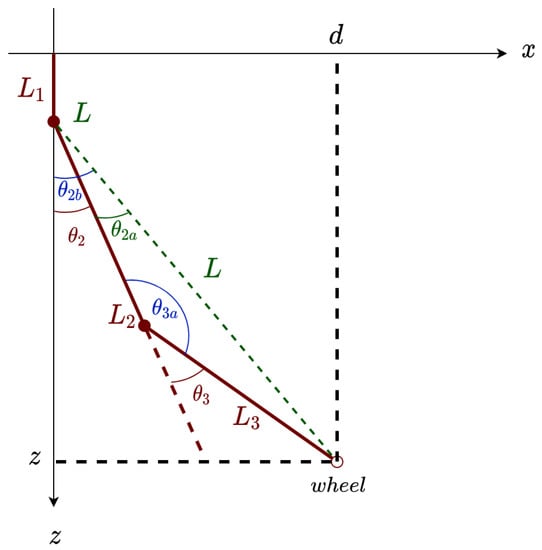
Figure 14.
Inverse kinematics representation.
Finally, by applying a profile generator to the desired positions, similar to the one presented in [16], and using the previously mentioned Inverse Kinematics implementation as input to the previously presented controllers solutions, the system can now produce the desired wheel positions. The full controller block diagram is presented in Figure 15.
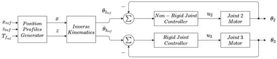
Figure 15.
Complete control block diagram.
3. Results
In order to test the controllers and validate the results obtained in simulation, a test set of points was defined that was applied to the leg trajectory planner. The tested points are shown in Table 4.
Table 4.
Set of positions.
Graphically, Figure 16, Figure 17 and Figure 18 illustrate the leg’s physical behavior when some test sets of reference points are required to the system. As the graphical representations demonstrate, the desired points can be reached, although with some associated error. Analyzing more specifically each of the tests carried out, it is possible to obtain the following errors presented in Table 5 and Table 6, namely the average and maximum absolute errors in x, z, and , as well as the maximum error of each in steady state (SS).
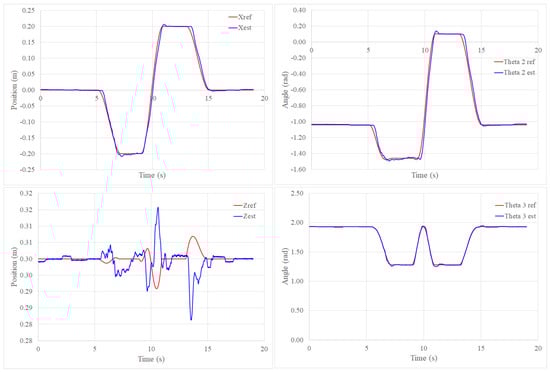
Figure 16.
Trajectory Following Results—Test Set 1.
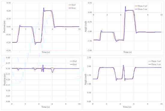
Figure 17.
Trajectory Following Results—Test Set 2.
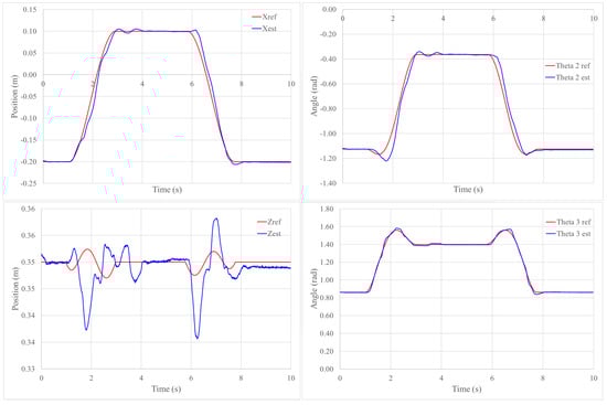
Figure 18.
Trajectory Following Results—Test Set 3.
Table 5.
Errors in Positioning.
Table 6.
Errors in Positioning.
Evaluating the registered error values, the maximum average error in positioning in x is 0.00042 m, in z is 0.00046 m, in is 0.00207 rad, and in is 0.00016 rad. Regarding the maximum absolute error values, there are some larger values, in x is 0.10211 m, in z is 0.04302 m, in is 0.51481 rad, and in is 0.14368 rad. Finally, the maximum errors in steady state are in x is 0.00367 m, in z is 0.00238 m, in is 0.02158 rad, and in is 0.02268 rad. The average values are low, indicating that the maximum absolute error values are residual, and it can be analyzed that these values are obtained due to the overshoot of the system when the final time () is set to 0.5 s. In steady state the maximum errors are below 0.3 cm in x and z and lower than 0.02 rad in and . Regarding the final time to reach the desired value, which is also a variable that can be changed, the three test sets use different values, confirming that the positioning can take different settling times. However, it is also noticeable that the error decreases when this time is increased, not requiring as much performance in the movement of the joints.
Another aspect is the smooth positioning profiles created to move the joints without requiring too much initial speed or torque, and sudden movements, which can damage the mechanical construction or the electrical powering elements.
4. Conclusions and Future Work
Throughout this article, a robotic legged-wheeled system designed to be applied on a hybrid mobile robot locomotion system was presented. Theoretically, all steps of the mechanical and electronic designs, physical modeling of the system, control of each used joint, and the combined control of both were presented. Besides this, a physical prototype was built, which allowed the practical test of the theoretically developed controllers. Thus, it is considered that the entire development structure was successfully achieved.
The modeling phase was also considered successfully reached, being able to obtain a model of each of the joints with a relatively high degree of precision, as can be verified by the obtained data, when compared with the simulation one.
Regarding the controller, it can be seen in practice that the developed design presented successful results, achieving a maximum positioning error in steady state of approximately 0.37 cm. The smooth profiles are a valuable asset in the preservation of the equipment integrity and also to avoid sudden movements.
Regarding the future work, the authors intend to conduct more tests, in order to improve the obtained models, especially at low frequencies, in which the model does not fit so well. Another relevant point is that this system will be applied, in the near future, in a configuration of a hybrid mobile robot to test its full capacity, predictably in a quadruped robotic configuration, like the CAD rendering presented in Figure 19.
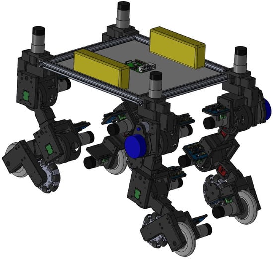
Figure 19.
Quadruped configuration CAD rendering.
Following the latter, the developed software structure will have to be expanded to allow the use of several legs simultaneously, in order to allow the control of the vehicle. Considering the possible future mechanical improvements, it will also be important to add at least 1 more DOF, on the hip, in order to allow rotation along the x axis.
Author Contributions
Conceptualization, V.H.P. and P.C.; methodology, V.H.P., J.G. and P.C.; software, P.C. and V.H.P.; validation, V.H.P. and P.C.; investigation, V.H.P.; writing—original draft preparation, V.H.P.; writing—review and editing, V.H.P., J.G. and P.C. All authors have read and agreed to the published version of the manuscript.
Funding
This work is financed by National Funds through the Portuguese funding agency, FCT - Fundação para a Ciência e a Tecnologia, within project UIDB/50014/2020.
Conflicts of Interest
The authors declare no conflict of interest.
References
- Schwarz, M.; Rodehutskors, T.; Droeschel, D.; Beul, M.; Schreiber, M.; Araslanov, N.; Ivanov, I.; Lenz, C.; Razlaw, J.; Schüller, S.; et al. NimbRo Rescue: Solving disaster-response tasks with the mobile manipulation robot Momaro. J. Field Robot. 2017, 34, 400–425. [Google Scholar] [CrossRef]
- Kashiri, N.; Baccelliere, L.; Muratore, L.; Laurenzi, A.; Ren, Z.; Hoffman, E.M.; Kamedula, M.; Rigano, G.F.; Malzahn, J.; Cordasco, S.; et al. CENTAURO: A hybrid locomotion and high power resilient manipulation platform. IEEE Robot. Autom. Lett. 2019, 4, 1595–1602. [Google Scholar] [CrossRef]
- Hutter, M.; Gehring, C.; Jud, D.; Lauber, A.; Bellicoso, C.D.; Tsounis, V.; Hwangbo, J.; Bodie, K.; Fankhauser, P.; Bloesch, M.; et al. ANYmal—A highly mobile and dynamic quadrupedal robot. In Proceedings of the 2016 IEEE/RSJ International Conference on Intelligent Robots and Systems (IROS), Daejeon, Korea, 9–14 October 2016; pp. 38–44. [Google Scholar]
- Bjelonic, M.; Sankar, P.K.; Bellicoso, C.D.; Vallery, H.; Hutter, M. Rolling in the Deep–Hybrid Locomotion for Wheeled-Legged Robots using Online Trajectory Optimization. IEEE Robot. Autom. Lett. 2020, 5, 3626–3633. [Google Scholar] [CrossRef]
- Eich, M.; Grimminger, F.; Bosse, S.; Spenneberg, D.; Kirchner, F. Asguard: A hybrid-wheel security and sar-robot using bio-inspired locomotion for rough terrain. In Proceedings of the ROBIO 2008, Bangkok, Thailand, 22–25 February 2009; pp. 774–779. [Google Scholar]
- Shi, Q.; Miyagishima, S.; Konno, S.; Fumino, S.; Ishii, H.; Takanishii, A.; Laschi, C.; Mazzolai, B.; Mattoli, V.; Dario, P. Development of the hybrid wheel-legged mobile robot WR-3 designed to interact with rats. In Proceedings of the 2010 3rd IEEE RAS & EMBS International Conference on Biomedical Robotics and Biomechatronics, Tokyo, Japan, 26–29 September 2010; pp. 887–892. [Google Scholar]
- Freitas, G.; Lizarralde, F.; Hsu, L.; Paranhos, V.; Dos Reis, N.R.S.; Bergerman, M. Design, modeling, and control of a wheel-legged locomotion system for the environmental hybrid robot. In Proceedings of the IASTED International Conference, Pittsburgh, Penn, 7–9 November 2011; pp. 7–9. [Google Scholar]
- Chen, S.C.; Huang, K.J.; Chen, W.H.; Shen, S.Y.; Li, C.H.; Lin, P.C. Quattroped: A leg–wheel transformable robot. IEEE/ASME Trans. Mechatron. 2013, 19, 730–742. [Google Scholar] [CrossRef]
- Kim, Y.S.; Jung, G.P.; Kim, H.; Cho, K.J.; Chu, C.N. Wheel transformer: A wheel-leg hybrid robot with passive transformable wheels. IEEE Trans. Robot. 2014, 30, 1487–1498. [Google Scholar] [CrossRef]
- Zheng, C.; Liu, J.; Grift, T.E.; Zhang, Z.; Sheng, T.; Zhou, J.; Ma, Y.; Yin, M. Design and analysis of a wheel-legged hybrid locomotion mechanism. Adv. Mech. Eng. 2015, 7, 1687814015616908. [Google Scholar] [CrossRef]
- Qiao, G.; Song, G.; Zhang, Y.; Zhang, J.; Li, Z. A wheel-legged robot with active waist joint: Design, analysis, and experimental results. J. Intell. Robot. Syst. 2016, 83, 485–502. [Google Scholar] [CrossRef]
- Hu, W.; Li, G.; Sun, Y.; Jiang, G.; Kong, J.; Ju, Z.; Jiang, D. A review of upper and lower limb rehabilitation training robot. In International Conference on Intelligent Robotics and Applications; Springer: Berlin/Heidelberg, Germany, 2017; pp. 570–580. [Google Scholar]
- Hu, J.; Hou, Z.; Zhang, F.; Chen, Y.; Li, P. Training strategies for a lower limb rehabilitation robot based on impedance control. In Proceedings of the 2012 Annual International Conference of the IEEE Engineering in Medicine and Biology Society, San Diego, CA, USA, 28 August–1 September 2012; pp. 6032–6035. [Google Scholar]
- Wu, J.; Gao, J.; Song, R.; Li, R.; Li, Y.; Jiang, L. The design and control of a 3DOF lower limb rehabilitation robot. Mechatronics 2016, 33, 13–22. [Google Scholar] [CrossRef]
- Feng, Y.; Wang, H.; Vladareanu, L.; Chen, Z.; Jin, D. New Motion Intention Acquisition Method of Lower Limb Rehabilitation Robot Based on Static Torque Sensors. Sensors 2019, 19, 3439. [Google Scholar] [CrossRef] [PubMed]
- Pinto, V.H.; Gonçalves, J.; Costa, P. Towards a More Robust Non-Rigid Robotic Joint. Appl. Syst. Innov. 2020, 3, 45. [Google Scholar] [CrossRef]
- Pinto, V.H.; Gonçalves, J.; Costa, P. Modeling and Control of a DC Motor Coupled to a Non-Rigid Joint. Appl. Syst. Innov. 2020, 3, 24. [Google Scholar] [CrossRef]
- Vaccaro, R.J. Digital Control: A State-Space Approach; McGraw-Hill Higher Education: New York, NY, USA, 1995. [Google Scholar]
- Van Loan, C. Computing integrals involving the matrix exponential. IEEE Trans. Autom. Control 1978, 23, 395–404. [Google Scholar] [CrossRef]
- Ackermann, J. The design of linear control systems in the state space. At-Automatisierungstechnik 1972, 20, 297–300. [Google Scholar]
Publisher’s Note: MDPI stays neutral with regard to jurisdictional claims in published maps and institutional affiliations. |
© 2021 by the authors. Licensee MDPI, Basel, Switzerland. This article is an open access article distributed under the terms and conditions of the Creative Commons Attribution (CC BY) license (http://creativecommons.org/licenses/by/4.0/).