
Research on Low-Speed Driving Model of Ultrasonic Motor Based on Beat Traveling Wave Theory


State Key Laboratory of Mechanics, Control of Mechanical Structure, Nanjing University of Aeronautics and Astronautics, Nanjing 210016, China
*
Author to whom correspondence should be addressed.
Actuators 2021, 10(11), 304; https://doi.org/10.3390/act10110304
Submission received: 16 October 2021
/
Revised: 10 November 2021
/
Accepted: 12 November 2021
/
Published: 19 November 2021
(This article belongs to the Section Aircraft Actuators)
Abstract
:This paper proposes a driving method, the superimposed pulse driving method, that can make an ultrasonic motor run at a low speed. Although this method solves the periodic oscillation of speed in a traditional low-speed driving motor, it still has a small periodic fluctuation, which affects the stability of the speed. To reduce the fluctuation rate of the motor speed, the structure model and driving model of the motor are established, based on the theory of a beat traveling wave, and the motion characteristics of the particle point are analyzed in this paper. The simulation curve of the motor speed is obtained according to the stator and rotor contact model and the transfer model. The research shows that the driving method introduced in this paper causes the stator surface to generate a traveling beat wave, and the driving end of the stator generates an intermittent reciprocating vibration and drives the rotor rotation, which is the mechanism of low-speed operation when the driving method is used to drive the motor, as well as the reason for the periodic fluctuation of the motor speed. To improve the speed stability, this paper controlled the output performance of the motor by changing the two control variables—prepressure and frequency difference—and concluded that the variation trend of the average speed and speed volatility were consistent with the variation trend of the motor’s average speed determinant and the speed volatility determinant, respectively, which is verified by the velocity measurement experiment and the vibration measurement experiment. These insights lay the theoretical foundation for the velocity adjustment and stability optimization and, finally, the application of the new driving method is prospected.
1. Introduction
The single-gimbal control moment gyro (SGCMG) is the main spacecraft attitude controller [1,2]. Considering the wide application of satellites in scientific research and commercial and military fields, the attitude control capability of satellites with high precision and high stability is important. The accuracy and stability of the control moment gyro (CMG) are determined by the gimbal’s angular velocity [3,4]. The existing framework of the CMG electromagnetic motor servo system is used by the harmonic reducer driving [5] with a slow system response and small power-to-weight ratio, but the fixed-angle locking power consumption and electromagnetic radiation do not overcome these shortcomings. These defects can lead to the CMG framework producing a “lag” phenomenon [6], and the interference phenomenon will cause instability in the operation of the system. With the improvement of maneuverability, stability, and the integration of the spacecraft, such as space satellites, it is necessary to find a new power source to make up for the aforementioned deficiencies. Compared with the electromagnetic motor, the traveling wave rotary ultrasonic motor (TRUM) has the following characteristics: small size, light weight, high torque at low speeds, and no electromagnetic interference [7]. These unique characteristics are concerns of the aviation field. Therefore, the unstable operation of the system can be solved by replacing the electromagnetic motor to control the speed of the CMG frame with the ultrasonic motor.
The TRUM is a complicated nonlinear coupling system, and the speed and speed stability of the motor are closely related to the contact interface between the stator and rotor. There are many factors affecting the contact interface, such as structural parameters, material parameters, load torque, driving power supply voltage, and prepressure and driving frequency. The last two factors—on the output characteristics of the motor—are particularly prominent. The prepressure determines the contact state of the stator and rotor, which has a profound influence on the dynamic characteristics of the stator, the friction and wear characteristics of the rotor, and the mechanical characteristics of the ultrasonic motor. The driving frequency range of the traveling wave ultrasonic motor is determined by the resonant frequency of the stator. By adjusting the driving frequency of the traveling wave ultrasonic motor, the difference between the driving frequency and the mechanical resonant frequency can be changed and, thus, speed regulation can be achieved. Compared with the phase difference and voltage regulation, a small range of frequency regulation can achieve linear speed regulation [8]. Many researchers regard the influence of the aforementioned factors on the speed and speed stability of the ultrasonic motor as research content. Chen et al. [9] studied the influence of prepressure on the key performance of the traveling wave ultrasonic motor through the simulation and experiment of the motor model. Mcfarland et al. [10] control the motor by applying different load torques, prepressure, and piezoelectric driving voltages to obtain the parameters of the speed, input power, output power, and efficiency to obtain the prepressure and height of the stator teeth when the motor achieves the best performance. Chau et al. [11] use the pulse width modulation and neural fuzzy control to control the speed trajectory of the sinusoidal curve of the motor. Kobayashi et al. [12] use the method of adjusting the driving frequency via the sampled-data H∞ control to realize the speed trajectory control of the trapezoidal wave curve.
The optimization of the aforementioned control variables is realized on the basis of the normal speed; however, the SGCMG framework requires operation at a low speed or an ultralow speed, and the speed regulation ratio needs to reach 1000:1 [13]. Therefore, the ability of the ultrasonic motor to work at an ultralow speed becomes the prerequisite to replacing the electromagnetic motor and to accurately adjusting the attitude of the satellite. To achieve this goal, some scholars have proposed a microstepping driving method to control the ultrasonic motor [14,15,16,17,18]. Omura et al. [14] realized the low-speed control of the traveling wave ultrasonic motor by adjusting the voltage and phase. Shi et al. [15] selected the driving voltage of the motor as the control variable and adopted a fuzzy PID control to adjust it in real time to realize the low-speed control of the linear motor. Senjyu et al. [16] adopted the motor speed control method, combining frequency conversion speed regulation and DC power PWM control to achieve the highest efficiency speed regulation control. Chen et al. [17] managed the motor speed and displacement by controlling the number and driving period of the driving wave. Wang et al. [18] controlled the motor speed and displacement by stimulating the first longitudinal vibration and the second bending vibration of the motor, and by controlling the number of driving waves, driving voltages, and the prepressure and driving frequencies. Although the microstep driving method can realize the ultralow speed operation of the motor, the speed will have a large periodic oscillation [19], which has a considerable impact on the stability of the motor speed, but there is limited relevant literature that can solve the aforementioned problems.
To eliminate the velocity fluctuation caused by the driving mechanism, a new driving method—the superimposed pulse driving method—was proposed [19], and the experimental results show that, compared with the microstepping driving method, a new driving method obviously reduces the inertia the mechanical system brings to the motor speed of the adverse impact of the cyclical shocks and greatly reduces the volatility of their speed, and the specific driving principle has been described in detail in the literature [19]. When the new driving method is used to drive the motor, although the motor speed does not experience periodic oscillation, it still has a small amplitude of periodic jitter phenomenon, which has an impact on the speed stability, so it is necessary to establish a mathematical model to study and discuss its mechanism. So far, a great deal of research using different methods has been published in the literature on the modeling and simulation of the TRUM.
In this paper, the two variables—prepressure and frequency difference—between the driving frequency and resonant frequency are considered the input variables, and the driving model of the ultrasonic motor is established, which lays a theoretical foundation for speed regulation and stability optimization.
This paper is divided into nine sections. In Section 2, the equivalent model of the motor stator is established and the expression of the resonant frequency of the stator under prepressure is obtained. In Section 3, the theoretical model, based on the superimposed pulse driving method, is established and the driving mechanism is described. In Section 4, the contact model and transfer model of the stator and rotor, based on the superimposed pulse driving method, are established. In Section 5, the motion characteristics of the particle points on the stator surface in the three regions of the driving method are simulated, and the trajectory and displacement curves of the particle point in vertical directions are obtained when the beating wave propagates on the stator surface. In Section 6, by changing the prepressure and frequency difference, the instantaneous speed simulation curve of the motor, and the simulation curve that reflects the expression of the determining factor of the motor’s average speed and fluctuation, are drawn. In Section 7, the vibration measurement experiments are carried out to verify the correctness of the simulation model theory. In Section 8, the univariate and multivariable motor speed control is carried out, the motor speed measurement chart and the trend chart of the characteristic variables are drawn, and the conclusions are given. At last, the experiment and simulation conclusions are summarized, and the prospective research ideas are stated.
2. Structure of the Stator
The stator is the core of the motor, and the change in the stator natural frequency and the particle point motion characteristics under prepressure can determine the output performance of the ultrasonic motor. Therefore, this paper uses the TRUM-60 as the research object and analyzes the influence of the stator structure on the natural frequency.
2.1. Equivalent Model and Stator
The stator of the traveling wave ultrasonic motor is composed of a piezoelectric ceramic and ring metal elastomer with teeth, as shown in Figure 1a. The role of the teeth is to increase the vibration amplitude of the stator and to improve the friction transmission efficiency of the stator and rotor without affecting the bending stiffness and natural frequency of the stator composite beam. To facilitate the analysis, the composite stator ring is expanded into an equal-straight beam in this paper, as shown in Figure 1b.
Because the back of the stator ring is affixed with piezoelectric ceramics, the stator ring is a composite beam, as shown in Figure 1c, and the distance from the upper surface of the composite beam to the neutral layer is as follows [20]:
where , and, additionally, denotes the number of teeth of the stator ring; denotes the ratio of the tooth height of the stator, , to the thickness of the elastic beam, ; denotes the ratio of the sum of the width of the stator’s grooves, , to the circumference of the stator, ; denotes the material density of the elastic beam; denotes the width of the elastic beam; and denote the tooth height and beam thickness of the elastic beam, respectively; and denote Young’s modulus and the shear modulus of the stator metal, respectively; and and denote the thickness and width of the piezoelectric ceramics, respectively. The Young’s modulus, , the average density, , the moment of inertia, , and the shear modulus of the composite beam, , are shown below [21]:
where .
2.2. Natural Frequency Analysis
The stator vibration, on the basis of the Timoshenko model theory, is analyzed in this paper, and the coupling equation is obtained according to the D’Alembert principle [22,23]:
where denotes the cross-sectional area; denotes the mass density of the beam material; denotes the load along the beam; denotes the shear correction coefficient; and denotes the bending angle between the beam axis and the x axis. According to the boundary conditions, the modal response of the beam with the modal order, , is shown below.
where , denotes the stator radius denotes the modal order of the stator vibration; denotes the natural frequency of the stator without prepressure; and denotes the response amplitude of the stator to the excitation. According to Newton’s second law, the vibration equation under prepressure can be described as:
where , denotes the vertical equivalent spring stiffness of the friction materials denotes the elastic modulus of the friction material denotes the length of the contact zone between the stator and rotor; and and denote the width and thickness of the friction material layer, respectively. Submitting Equations (2) and (4) into Equation (5), the stator resonant angular frequency, , under prepressure can be simplified as:
Prepressure is one of the key parameters that limits the performance of the ultrasonic motor, and it can affect the resonant frequency of the stator [8]. The frequency characteristic analyzer will be used to measure the resonant frequency of the stator under different prepressures to verify the reliability of Equation (5) in Section 7.
2.3. Amplitude Analysis under Prepressure
The stator vibration waveform is formed by the superposition of the standing waves excited by two groups of piezoelectric plates, and the stator is a linear system, so the amplitude of the stator vibration only needs to consider the amplitude generated by the excitation of one group of piezoelectric plates. According to the piezoelectric equation [8], the maximum particle point amplitude without prepressure can be described as:
where , denotes the length of a piezoelectric partition denotes the sinusoidal voltage applied vertically to the piezoelectric plate; denotes the strain constants of the piezoelectric ceramic materials denotes the flexibility factor denotes the damping ratio of the stator; and denotes the driving angular frequency of the piezoelectric ceramic vibration. The prepressure affects the resonant frequency of the stator and has a great influence on the amplitude of the stator particle point [24]. The amplitude of the stator decreases gradually with the increase in prepressure. The relationship between the particle point amplitude of the stator surface, , and the prepressure under different prepressures, , can be described as:
The amplitude of the stator under different prepressures will be measured by using the scanning laser vibration measurement system in Section 7, and the values of the constants, and ς, in Equation (8), can be obtained by curve fitting.
3. Theoretical Analysis of Ultrasonic Motor Driving Method
3.1. Stator Particle Point Setting
There is a layer of relatively soft friction material between the stator and rotor of the ultrasonic motor. When the ultrasonic motor works, the contour line of the stator surface is a sinusoidal wave shape because of the generation of traveling waves. Under the prepressure, because the material of the stator and rotor is hard and the prepressure is small, it can be assumed that there is no contact deformation between the stator and rotor. Only the friction layer produces corresponding deformation, and the deformation of the friction layer is consistent with the contour line of the stator surface [25,26]. The contact interface between the stator and rotor of the traveling wave ultrasonic motor is shown in Figure 2b.
When the motor is driven by the superimposed pulse driving method, the main objective of this paper is to detect the variation trend of the motor speed and speed fluctuation by changing the difference in the prepressure and the angular frequency.
The movement characteristics of the particle point (e.g., particle point Q in Figure 2) can reflect the variation in the motor speed and the speed of the volatility trends because of the speed of the rotor and the elliptical motion of the stator particle point transfer. In particular, the motion characteristics of the wave peak particle point (particle point H in Figure 2) have been in contact with the friction material of the rotor and can determine the output performance of the motor. It should be noted that particle point Q, defined in this paper, is any fixed particle point of the stator, and the abscissa position of the particle point does not change with time, while the abscissa position of the particle point, H, does, as shown in Figure 2c.
3.2. Partition Introduction to the Driving Method
One cycle of the superimposed pulse driving method is divided into three regions, namely, the traveling standing wave increasing region, , the traveling standing wave amplitude reduction region, , and the traveling standing wave amplitude increasing and decreasing transition region, , respectively, as shown in Figure 3.
3.2.1. Traveling Standing Wave Amplitude Reduction Region ()
According to the principle of mechanical vibration [17], before the A-phase of the stator is de-energized (the period before in Figure 3), the particle point, Q, on the stator near the equilibrium position, has a constant-amplitude vibration with driving frequency, , and the amplitude of . However, after the power is cut off (the period after in Figure 3), the particle point does not decay to the equilibrium position immediately. Instead, it vibrates near the equilibrium position with resonant frequency and decreasing vibration amplitude. The particle point of the stator B-phase vibrates at a constant amplitude, with the driving frequency and the vibration amplitude, , near the equilibrium position. The whole aforementioned process is in .
3.2.2. Traveling Standing Wave Amplitude Increasing and Decreasing Transition Region ()
Before the amplitude of particle point Q decays to the equilibrium position, the A-phase of the stator starts to charge up, and the particle point on the stator will vibrate back and forth with increasing amplitude near the equilibrium position. The whole aforementioned process is in .
3.2.3. The Traveling Standing Wave Increasing Region ()
According to the working principle of the traveling wave ultrasonic motor, the piezoelectric ceramics are driven by a sinusoidal voltage with a phase difference of 90 degrees. Because of the motor stator for the underdamped system, the amplitude of the stator for the A-phase particle points maintain . However, after the B-phase of the stator is charged, the particle point, Q, will experience a reciprocating vibration with increasing amplitude near the equilibrium position, and the two-phase standing waves with the same oscillation frequency, but different vibration amplitudes will be superimposed to synthesize the traveling wave and to propagate on the stator. The whole aforementioned process is in .
3.3. Motion Characteristics of the Stator Particle Points in
According to the theory of free vibration and the forced vibration of the underdamped system [23], the modal responses, and , in the vertical direction of the stator’s two phases are obtained as follows (see the electronic Supplementary Material for the specific derivation formulas):
where denotes the response amplitude of the stator to the excitation of the A-phase. Additionally, denotes the response amplitude of the stator to the excitation of phase A, and ,, and denote the initial response phase of the stator to the excitation of the A-phase in the three regions (, , and ) of the driving method. Further, ,,, and denote the shift angle of the phase difference (see the electronic Supplementary Material for specific derivation formulas).
According to the superposition principle, the vertical and tangential displacements of particle point Q can be described as:
According to the rotation vector method, the amplitude, , of point Q in the vertical direction is expressed as follows:
where and denote the amplitude vectors of the stator two-phase mode function in the three regions of the driving method, respectively, and the expressions in the three regions of the driving method are as follows:
In Equation (12), ,, and denote the angular frequency difference, the initial time value, and the phase difference of the stator’s two phases, respectively. The expressions in the three regions of the driving method are as follows:
where , , and denote the angular frequency difference in the three regions of the driving method, respectively. In Equation (14), , , and also denote the shift angle of the phase difference (see the electronic Supplementary Material for the specific derivation formulas). When the motor is driven based on the superposition driving method, the expressions of the period of the beat traveling wave on the stator surface in the three regions of the driving method are shown as follows (see Equation (A9) in Appendix A):
The tangential velocity of a particle can be expressed as:
where and denote the amplitude and phase angle of the tangential velocity of the particle, respectively, and the expressions are demonstrated in the three regions of the driving method.
where
3.4. Motion Characteristics of Particle Point H of the Stator Wave Crest
When the stator particle point is at the wave peak, the vertical velocity is zero, which is [8]. Substitute Equation (11) into the equation to obtain the x-coordinate of particle point H for the stator wave crest, as follows:
Substitute Equation (20) into Equation (11) to obtain the vertical displacement of the particle point at the wave peak:
Substituting Equation (20) into Equation (11), the tangential velocity of the particle at the wave peak is expressed as:
3.5. The Elliptical Trajectory of the Stator Particle Point Q
As shown in Figure 4a, the coordinate of any point in the coordinate system is in the coordinate system .
The general equation of the ellipse obtained by combining Equation (11) with Equation (A13) in Appendix B is shown as follows:
where
According to Equation (A8) in Appendix A, the determining factor for the direction of the elliptical motion is:
where
Additionally, and denote the determinants of the motion direction of the ellipse in and , respectively, as shown in Figure 4b,c. In each beat wave period, the elliptical motion of a particle will have two phases of rotation in the clockwise direction and counterclockwise direction, and the time for both phases is half of the beat wave period. Notably, is the determining factor of the elliptical motion direction in , as shown in Figure 4d. Because the propagation waveform on the stator surface is a traveling wave with changing amplitude—instead of the beat traveling wave—particle Q rotates clockwise around the center point of the ellipse.
4. Stator and Rotor Contact Model and Transfer Model
Contact force is generated when the stator and rotor contact each other. It is necessary to conduct contact modeling to evaluate the contact force. Friction materials are used to adhere to the surface of the rotor to improve the interfacial force of the motor. When the rotor is pressed against the stator surface, a deformation occurs on the friction material surface. When the stator is excited, the traveling waves are excited on the surface of the stator, and the upper surface takes on a sine-wave shape [27]. Because of the different elastic moduli of the friction materials and the stator, the contact surface is considered the Hertz contact model of the rigid stator and flexible rotor [25]. The contact interface between the stator and rotor of the TRUM is expanded in two dimensions along the circumferential direction, as shown in Figure 5.
The peak of the wave will penetrate into the friction material, and the contact area is not a point, but a region. At this point, the two resultant forces, the normal force and the tangential force, act on the contact surface. The contact model and transfer model are analyzed below.
4.1. Analysis of Stator and Rotor Contact Model
When the motor is driven by a superimposed pulse driving method, the stator will excite mode . According to the Hertz contact theory, the stator is a cylinder with an equal-radius curvature at the peak of the row wave. When the rotor is assumed to be an elastic plane, the contact area length of the contact interface between the motor and the rotor is under the action of prepressure . The contact position of the interface between the stator and rotor changes with time, along with the shape, and the relative motion and the interaction force of the contact area between the stator and rotor, so the particle point amplitude of the stator wave peak will change with time. According to the Hertz contact theory, the equivalent curvature diameter, , is expressed as follows [26]:
where denotes the equivalent radius of the stator, and the contact area length, , of the contact interface between the stator and rotor under the action of prepressure, , is shown below [26]:
where , and, additionally, denotes the parameters related to the material properties; and and denote the Poisson’s ratio of the stator to the friction material, respectively [26,28]. Combining Equation (20) and Equation (26), the x-coordinate expression of the contact critical point between the motor stator and rotor in one period of the superimposed pulse driving method is shown as follows:
As shown in Figure 5, stands for the distance between the lower surface of the friction material and the central axis of the waveform of the stator surface without deformation. This paper adopts instead of to express the contact range, which will be more conducive to describing the contact degree between the stator and rotor. Substitute Equation (27) into Equation (11) to obtain the expression shown below.
The tangential velocity of the contact critical point is shown as follows:
Because the pressure distribution function is proportional to the vertical displacement of the stator particle point [29], the obtained expression is shown as follows:
The expression derived from Hooke’s law [30] is shown below.
Combining Equation (28), Equation (30), and Equation (31), the pressure distribution functions of the three regions of the superimposed pulse driving method are shown as follows:
4.2. Transfer Model Analysis of the Stator and Rotor
4.2.1. Analysis of the Nonslip Point
The force of the friction is generated between the stator and rotor and drives the rotor to rotate under prepressure in Figure 5, and the tangential velocity of the particle points on the contact surface of the stator and rotor is set as . and are set as edge contact points, and the tangential velocity of the two particle points is set as . is set as the contact point of the wave crest, and the tangential velocity of the particle point is set as . Additionally, and are set as the two contact points with the same tangential velocity on the contact surface of the stator and rotor, that is, . Because there is no relative sliding between the stator and friction material here, the stator particle point has no hindering or driving effect on the rotor. This point is also called the nonsliding point, which is the critical point [31] dividing the driving area and the braking area, and the speed at this point is set as .
4.2.2. Position Value of Nonsliding Point
Instantaneous tangential velocities of the stator particles in the three regions of the driving method are drawn according to Equation (16) and are shown in Figure 6.
The abscissa of the velocity peaks and troughs in the three regions of the driving method is obtained according to the aforementioned equation as follows:
When the tangential velocity of the nonsliding point is set to , the expression of the abscissa of the nonsliding point is obtained according to the definition of the inverse function as follows:
According to the definition of the inverse, the range of the inverse tangent function is. However, because the wave peak particle point propagates on the stator surface with a wavelength of , the abscissa range of the nonsliding point is set as , according to Figure 4. On the basis of the fact that the x-coordinate of the nonsliding point, X, is the value between the x-coordinate of the wave peak (Equation (34)) and the x-coordinate of the critical point of the contact surface (Equation (27)), the expression of the nonsliding point corresponding to the only nonsliding point of the tangential velocity is as follows:
4.2.3. Analysis of Driving Torque
Because Coulomb’s friction is considered friction force, , this one can be expressed by Equation (36) [32]:
where
When the traveling wave propagates on the stator surface, the velocity direction remains the same [8]. However, when the beat traveling wave propagates on the stator surface, the tangential velocity direction of the particle point, H, of the wave peak in contact with the rotor changes periodically. Taking the nonsliding point as the critical point, the braking zone and driving zone of the transfer model are divided according to the aforementioned definition. In this paper, when the velocity direction of the nonsliding point is to the right, it is positive, and when the velocity direction of the nonsliding point is to the left, it is negative. Additionally, when the velocity direction of the nonsliding point is to the left, the transfer model of the stator and rotor is a reverse nonsliding point transfer model. When the velocity direction of the nonsliding point is to the right, the transfer model of the stator and rotor is a forward nonsliding point transfer model. The following is a detailed analysis of the two transfer models.
a. Forward Nonslip Point Transfer Model
In this paper, the tangential velocity, , of the edge contact point, the tangential velocity, , of the crest contact point, and tangential velocity zero are taken as special points of the stator particle point, and the tangential velocity, , of the nonsliding point is compared with that of the nonsliding point and then inserted into Equation (37) to obtain the eight transfer models shown in Figure 7.
The transfer model in Figure 7 determines the direction of friction according to the calculation results of the formulas, , and . When the tangential velocity, , of the edge contact point or the tangential velocity, , of the crest contact point are greater than the tangential velocity, , of the nonsliding point, this region is the driving zone (the area of the plus sign), and vice versa is the braking zone (the area of the minus sign).
b. Reverse Sliding Point Transfer Model
A same modeling method as the forward nonslip point transfer model is used to obtain the eight reverse nonsliding point transfer models, as shown in Figure 8.
When the tangential velocity, , of the edge contact point, or the tangential velocity, , of the crest contact point are less than the tangential velocity, , of the nonsliding point, this region is the driving zone (the area of the plus sign), and vice versa is the braking zone (the area of the minus sign). According to the torque balance equation, the expression is shown as follows:
where ,,, denotes the resultant force of friction, denotes the loading moment, denotes the moment of inertia for the rotor, and denotes the angular velocity of the rotor’s rotation.
5. Simulation of Motion Characteristics of the Stator Particle Point
According to the aforementioned contact model of the stator on the surface of the particle point, the movement characteristics can reflect the output performance of the motor, and the following will use MATLAB to simulate the motion trajectory, tangential velocity, and vertical displacement of the stator particle simulation curve.
5.1. Motor Simulation Parameter Setting
This paper makes use of TUSM-60 to conduct the model simulation, and the parameters of the ultrasonic motor are in Table 1.
5.2. Simulation of Particle Point Motion Characteristics
5.2.1. Simulation of Particle Point Motion Characteristics in
Particle point Q is selected as the reference point below, and the number of periodic pulses, , and the single-phase output pulses, , are set to 100 and 55, respectively. When the pressure is set to N, the difference in the angular frequency is set to rad/s, according to Equation (23), and the elliptical trajectory of particle point Q is shown in Figure 9.
According to Equation (12) and Equation (24), the simulation curves of the vertical displacement of particle point Q, , and the determining factor equation of the elliptical motion direction, , are obtained, respectively.
As shown in Figure 10, there is one beat period in is , and one beat period is divided into four-beat miniperiods, , on average (see Figure 9). The particle point Q moves clockwise in the first and fourth beat miniperiods ( and ), while the middle two small periods of the beat wave ( and ) move counterclockwise. In this paper, the clockwise direction is set as the positive direction, and the counterclockwise direction is set as the negative direction. It can be found that the change trend of the positive and negative signs of the determinant value of Formula is consistent with the rotation direction of particle Q in Figure 11. Additionally, the change trend for the value of the determining factor of the elliptical motion direction, , and the tangential velocity of particle point H, , at the wave peak is also consistent.
5.2.2. Simulation of the Particle Point Motion Characteristics in
Particle point Q is still selected as the reference point below. The number of periodic pulses, , the number of single-phase output pulses, , the prepressure, , and the angular frequency difference, , are consistent with those set above (the specific content is located in Section 5.2.1). The elliptical trajectory of particle point Q is shown in Figure 12.
According to Equations (11) and (24), the simulation curves of the vertical displacement of particle point Q, , and the determining factor equation of the elliptical motion direction, , are obtained, respectively.
As shown in Figure 13, there is one beat period in is , and a beat period is divided into four-beat miniperiods, , on average (see Figure 12). The particle point Q moves counterclockwise in the first two stages of the beat miniperiod ( and ), while the other two small periods of the beat wave ( and ) move clockwise. According to the change in the particle point’s motion and the positive and negative signs of the result of Formula in Figure 14, the change in the positive and negative signs of the determinant value of Formula is consistent with the rotation direction of particle Q in Figure 14. Additionally, the change in the trend of the value of the determining factor of the elliptical motion direction, , and the tangential velocity of particle point H, , at the wave peak, is also consistent.
5.2.3. Simulation of Particle Point Motion Characteristics in
Particle point Q is still selected as the reference point below. The number of periodic pulses, and the number of single-phase output pulses, are set to 100 and 75, respectively, and the prepressure, , and the difference in the angular frequency, , are consistent with those set above (the specific content is located in Section 5.2.1). The elliptical trajectory of particle point Q is shown in Figure 15.
According to Equations (11) and (24), the simulation curves of the vertical displacement of particle point Q, , and the determining factor equation of the elliptical motion direction, , were obtained, respectively.
Although the beat period of the vertical displacement is , as shown in Figure 16, the beat vibration of the stator surface is not caused by the frequency difference but by the constant change in the amplitude of the stator’s two phases. When the stator surface is in , as the stator surface propagates in the form of traveling waves, particle point Q does not change the rotation direction intermittently but keeps moving in a clockwise elliptical trajectory, which is consistent with the positive value of formula in Figure 17. Additionally, the change trend for the value of the determining factor of the elliptical motion and the tangential velocity of the particle point H at the wave peak is also consistent in Figure 17.
5.3. Simulation Characteristics of the Drive Method
From the waveform of the aforementioned simulation curve, it can be seen that the determining factor in any region of the superimposed pulse driving method can reflect the rotation direction of the particle point of the stator, as well as reflect the tangential velocity of the particle point at the peak of the wave. Because the friction material between the wave peak particle point and the rotor is always in contact, the tangential velocity and vertical displacement of the particle obtained by the contact model and the transfer model will directly affect the motor speed and the fluctuation of the speed. In the following, a series of expressions are obtained to reflect the output performance of the motor by changing the prepressure, , and frequency difference, , based on the characteristics of the determining factor of the direction of the elliptical motion in Section 6.
6. Simulation of the Motor Output Characteristics
6.1. Setting of Characteristic Variables
In this paper, four characteristic variables are set up to pave the way for the following analysis. The expression for the average of the motor speed is shown in Figure 18.
where denotes the instantaneous speed of the motor; and denotes the number of sampling points.
The expression for the motor speed volatility, , is shown below.
where denotes the variance of motor speed fluctuation, and the expression is shown below.
As shown in Figure 19, , and the instantaneous tangential velocity are defined as the forward velocity when the direction is to the right, and the backward velocity when the direction is to the left, in the three regions of the driving method. and denote the algebraic sum of and , respectively, and denotes the one-cycle time of the superimposed pulse driving method. denotes the time for the stator particle to rotate in the clockwise direction within , and denotes the time for the stator particle to rotate in the counterclockwise direction within .
According to Equations (11) and (24), the relationship between the determinants of the elliptical motion direction, , the tangential velocity of the peak particle point H, , and vertical displacement of the peak particle point H, , in the three regions of the driving method is obtained and shown as follows:
Since the rotor and the stator are in contact at the wave peak, the two parameters, the amplitude and the tangential velocity of the particle at the wave peak, jointly determine the rotor speed [8], and the two parameters are directly proportional to the rotor speed. According to Equation (42), the determining factor, , is the product of the above two parameters, so the determining factor determines the rotational speed of the rotor. According to the definition of the scale factor, when is larger, the clockwise rotation speed of the stator particle is larger, resulting in the greater forward velocity of the rotor, and vice versa. According to the definition of the average speed and volatility (Equations (39) and (40)), the expressions for the motor’s average speed determining factor, , and the speed fluctuation determining factor , which respectively reflect the average speed and fluctuation of the motor, are calculated as follows:
where and denote the algebraic sum of and , respectively.
6.2. Simulation of Motor Output Characteristics
The number of periodic pulses, , and the single-phase output pulses, , are set to 20 and 14, respectively, and the simulation of the motor instantaneous speed, , and the elliptical motion direction determination factor, , was performed under the condition that only one of the two parameters (angular frequency difference, , and prepressure, ) was changed, and the other parameter remained unchanged.
6.2.1. Simulation of Motor Speed and Determining Factor with Angular Frequency Difference
When the prepressure is set as N, and the angular frequency difference, , changes within the range of rad/s, the simulation curve is as shown in Figure 20.
After analyzing the simulation experiment according to the aforementioned definitions of the characteristic variables, the conclusion is as shown in Figure 21.
It can be seen from Figure 20b that decreases with the increase in the angular frequency difference, while increases with the increase in the angular frequency difference, . However, the cycle time for the superimposed pulse driving method, , remains almost constant. According to Equation (A14) in Appendix C.1, will decrease with the increase in the angular frequency difference. According to Equation (A16) in Appendix C.2, when , the determining factor for the rotation speed volatility, , will increase with the increase in the angular frequency difference, . Therefore, when the angular frequency difference, , changes, the variation trend for the average speed, , and the speed volatility, , were consistent with the variation trend for the motor’s average speed determinant, , and the speed volatility determinant, , respectively, as shown in Figure 21.
6.2.2. Simulation of Motor Speed and Determining Factor Change with Prepressure
When the angular frequency difference is set as rad/s, and the prepressure, , changes within the range of N, the simulation curve is as shown in Figure 22.
After analyzing the six groups of simulation experiments, according to the definition of the aforementioned variables, the conclusions were made and are as shown in Figure 23.
It can be seen from Figure 22b that decreases with the increase in prepressure, , and decreases with the increase in prepressure, , while the time of in one cycle of the superimposed pulse driving method remains almost unchanged. According to Equation (A14) in Appendix C.1, when increases with the increase in , increases with the increase in . According to Equation (A16) in Appendix C.2, when , the determining factor for the rotation speed volatility, , decreases with the increase in prepressure, . Therefore, when the prepressure, , changes, the variation trend for the average speed, , and the speed volatility, , were consistent with the variation trend of the motor’s average speed determinant, , and the speed volatility determinant, , respectively, as shown in Figure 23.
7. Vibration Test of Motor
7.1. Amplitude Analysis Experiment
As shown in Figure 24, the shell of the existing motor with prepressure is first cut into a small slot and part of the stator tooth surface is exposed. Then, the prepressure is changed by adjusting the motor’s adjustment nut. The PV-500-3D high-frequency scanning laser vibrometer, developed by the German company, Polytec, irradiates the scanning laser point on the tooth surface. Finally, after the prepressure adjustment is completed, the amplitude of the lower stator particle point under the 400 single-phase sinusoidal excitation is measured through the reflection of the tooth surface, as shown in Table 2.
When there is no prepressure on the stator, the amplitude measured, , is almost the same as the calculated result of Equation (7), and the data in Table 2 are inserted into Equation (8) and fitted to get the values for the constants, .
7.2. Prepressure Analysis Experiment
As shown in Figure 25a, to test the reliability of the calculation results of Equation (6), this paper adjusts the prepressure by adjusting the debugging nut of the motor and uses the frequency characteristic analyzer, FRA5087, to measure the resonant frequency of the stator changing with the prepressure under the 400 single-phase sinusoidal excitation. Then, the measured results of the experiment and theoretical calculation are compared to obtain the resonance frequency measurement graph with prepressure, as shown in Figure 25b.
According to Figure 25, the error value between the resonance frequency simulation result and the experimental test conclusion under prepressure is very small, which indicates that the calculation result of Equation (6) is reliable.
7.3. Single-Phase Power-Off Vibration Measurement Experiment
Because the motor stator is an underdamped system, when the stator single-phase power is cut off, the particle point on the stator will not immediately decay to the equilibrium position. Instead, it will experience a reciprocating vibration with the resonance frequency near the equilibrium position while its vibration amplitude is constantly decaying. To verify the correctness of this theory, as shown in Figure 26a, the signal generator sends out a pulse signal with a time length of , and then the sinusoidal signal, with a frequency of is amplified to by the power amplifier and applied to the A-phase piezoelectric ceramic plate of the stator to make the stator particle point vibrate with a standing wave and constant amplitude. Finally, the scanning laser vibrometer was used to measure the vertical velocity of the stator tooth particle point (point M in Figure 24) near the outage time point, , as shown in Figure 26b.
The vibration frequency of the particle point (point M) on the stator surface of the A-phase piezoelectric ceramic wafer is the driving frequency, ω_q (45 kHz), at the time period, T single, before the power failure. However, at the time period T_single redu, after the power failure, the amplitude of the particle point’s vertical velocity decreases continuously and the vibration frequency changes from the driving frequency, ω_q (45 kHz), to the resonance frequency, ω_n (39.703 kHz). Through a single-phase power-off vibration measurement experiment, it is verified that the stator forced-vibration frequency is the driving frequency, and the stator free-vibration frequency is the resonant frequency, which lays a theoretical foundation for the following two-phase power-off experiment.
In addition, since the motor stator is an underdamped system, the amplitude of free vibration decays exponentially. Therefore, this paper determines the damping ratio, ξ, in Table 1, according to the velocity attenuation rate of the particle point (point M) in the vertical direction.
7.4. Two-Phase Power-Off Vibration Measurement Experiment
To verify the correctness of the beat traveling wave period in Section 5, the experimental process is as follows: first, the sinusoidal signal, with a voltage of , and a frequency of 45 kHz, is applied to the B-phase piezoelectric ceramic plate of the stator to make the stator particle points vibrate with the standing wave and equal amplitude (blue line in Figure 27a), and then the sinusoidal signal with the same frequency and voltage amplitude, and a phase difference of 90 degrees, is applied to the A-phase piezoelectric ceramic plate of the stator (red line in Figure 27a). Finally, the A-phase piezoelectric ceramic chip is powered off at the moment of time point .
According to the experimental measurement, the vibration frequency of the stator tooth particle point (point M in Figure 24), before the outage time point, , is the driving frequency, (45 kHz), while after the outage time point , the envelope of the longitudinal velocity and amplitude of the particle point is displayed as a beat wave contour. According to Equation (15), the period of the beat wave is as follows:
As shown in Figure 27b, the beating wave period obtained from the vibration measurement experiment is, which is close to the calculation result of Equation (15). It verifies the correctness of the theory that, when standing waves of different frequencies and amplitudes are applied to the two phases of the motor, the beating traveling wave will be generated on the stator surface.
8. Experiment Research
8.1. The Establishment of the Experimental Platform
As shown in Figure 28, the experimental platform consists of a data acquisition device, a drive control board, and an upper computer. In this experiment platform, a high-precision encoder is used to measure the low speed of the motor, string is used to drag the weight in the outer ring of the torque plate, and the product of the pressure measured by the pressure sensor and the radius of the rotor is used to obtain the load moment.
8.2. Setting of Experimental Control Variables and Analysis of Experimental Results
The driving controller is composed of a control block and a driving block. The driving block used a four-phase push-pull circuit, and the control block used a single-chip microcomputer, DSP-TMS320F28335. The parameters listed in Table 3 are taken as an example to test the motor speed to verify the correctness of the aforementioned speed simulation conclusions.
8.3. Univariate and Multivariable Control Motor Experiments and Analysis of Experiments
Three groups of experiments were conducted to verify the correctness of the variation trend of the simulation curves in Figure 21 and Figure 23.
8.3.1. Open-Loop Control of Single Variable Variation
In the following experiment, only one control variable (prepressure, , or the angular frequency difference, ) was changed, and the other control variable remained unchanged.
a. Open-Loop Control of Angular Frequency Difference
In this group of experiments, the prepressure, , was set as N, and the range of the angular frequency difference, , was . The experimental conclusion is shown in Figure 30.
By comparing the analysis results in Figure 30 and Figure 21, it can be found that when the frequency difference changes, the experimental analysis results of the velocity and volatility are slightly higher than the simulation results because the assembly of temperature, air humidity, and coaxiality is not taken into account in the simulation process, but these factors can obviously affect the output characteristics of the motor. As shown in Figure 30, the change in the angular frequency difference, , the variation trend of the average speed, , and the speed volatility, , were consistent with the variation trend of the motor’s average speed determinant, , and the speed volatility determinant, , respectively, which is consistent with the conclusion of the simulation experiment results analysis in Figure 21.
b. Open-Loop Control of the Prepressure Change
In this group of experiments, the angular frequency difference, , was set as , and the range of prepressure, , was N. The experimental conclusion is shown in Figure 31.
By comparing the analysis results in Figure 31 and Figure 23, it can be found that when the prepressure changes, the experimental analysis results of the velocity and volatility are also slightly higher than the simulation results, also due to the fact that environmental factors and assembly errors are not taken into account in the simulation process. As shown in Figure 31, the change in prepressure, , the variation trend of the average speed, , and the speed volatility, , were consistent with the variation trend of the motor’s average speed determinant, , and the speed volatility determinant, , respectively, which is consistent with the conclusion of the simulation experiment results analysis in Figure 23.
8.3.2. Open-Loop Control of Multivariable Change
Six experiments were conducted under the premise that the two control variables had changed. The set values of the two variables are shown in Table 5.
The experimental platform controls the motor operation according to the variables in Table 5, and the experimental results are shown in the figure below.
According to the deduction of the contact model and the transfer model theory above, when one of the values of the two variables changes, or changes simultaneously, the two parameters (amplitude and tangential velocity of the particle) may become larger or smaller at the same time, or one may become larger and the other may become smaller. Because the above two parameters are proportional to the motor speed, and the deciding factor is the product of the two parameters, according to Equation (42), when the multivariate changes, the determining factor, , is also able to reflect the trend of the motor speed change. In order to prove the correctness of the conclusion, multivariable control experiments were carried out in this paper, as shown in Figure 32, when the two control variables of the angular frequency difference, , and prepressure, , change simultaneously, the variation trend of the average speed, , and the speed volatility, , were consistent with the variation trend of the motor’s average speed determinant, , and the speed volatility determinant, , respectively. Through the conclusion of this experiment, it can be concluded that whether changing the multivariable or the single variable, the determining factor can reflect the change trend of the motor speed and the fluctuation.
9. Conclusions
In this paper, the driving principle of the superimposed pulse driving method is introduced, and the motor can operate at a low speed through the characteristic of the method, which solves the periodic oscillation of the motor speed when the traditional method (microstep driving method) drives the motor. Because of the driving mechanism, the speed will also have a small range of periodic jitter. To improve the speed stability, this paper established a motor driving model based on the superimposed pulse driving method. After a simulation drawing, vibration measurement experiment, and speed test experiment, the following conclusions were obtained:
- According to the model of the stator structure with teeth, the relation of the stator resonant frequency with prepressure is obtained.
- By changing the control variable of the frequency difference, a theoretical analysis, simulation drawing, and vibration measurement experiment are carried out on the motion characteristics of the stator particle points, and, finally, the correctness of the theory of the beat traveling wave is proven, according to the conclusion.
- On the basis of the Hertz contact theory, to establish the contact model and transfer model of the stator and rotor, when the motor is driven by the superposition pulse drive method, the stator surface generates a traveling beat wave, which causes the driving end of the stator to experience an intermittent reciprocating vibration and drives the rotor rotation, which is the driving method when the drive motor realizes a low-speed running mechanism, and is the cause of motor speed cyclical fluctuations. To reduce the speed volatility, this paper changed the two control variables (prepressure and frequency difference), and when the angular frequency difference and prepressure changed in the range of and N, respectively—whether the motor speed was controlled by a single control variable or a multivariable control—the variation trend in the average speed, , and the speed volatility, , were consistent with the variation trend of the motor’s average speed determinant, , and thge speed volatility determinant, , respectively, which is verified by the velocity measurement experiment and the vibration measurement experiment, and lays a theoretical foundation for velocity adjustment and stability optimization.
- The significance of this study is that the researchers only needed to calculate the values of the two determinants to get the variation trend for the motor’s speed and volatility, and adjust the prepressure and driving frequency according to this trend to finally obtain the required results, thus avoiding tedious experiments and saving a lot of time for scientific research.
Supplementary Materials
The following are available online at https://www.mdpi.com/article/10.3390/act10110304/s1. Equation derivation of motion characteristics of the stator particle points in the three regions of the driving method.
Author Contributions
Conceptualization, W.Z. and S.P.; methodology, W.Z. and S.P.; software, L.C.; validation, S.P. and W.Z.; formal analysis, W.Z.; investigation, S.P.; resources, W.R. and X.H.; data curation, W.R. and X.H.; writing—original draft preparation, W.Z.; writing—review and editing, W.Z. and S.P.; visualization, W.Z.; supervision, S.P.; project administration, S.P.; funding acquisition, S.P. All authors have read and agreed to the published version of the manuscript.
Funding
This research was funded by National Natural Science Foundation of China, grant number 51575260 and by National Natural Science Foundation of China-Aerospace Advanced Manufacturing Technology Research Joint Fund integration project, grant number U2037603.
Data Availability Statement
The data presented in this study are available on request from the corresponding author. The data are not publicly available due to the experimental data in this paper are related to the aviation projects involving secrecy.
Conflicts of Interest
The authors declare no conflict of interest.
Appendix A
The two-phase modal response of the motor can be described as:
where and denote the response amplitudes of the two-phase excitation, respectively, and and denote the phases of the two-phase excitation, respectively. According to the superposition theorem, the displacement of the stator particle in the vertical direction and tangential direction are shown below.
Under the action of the beating traveling waves, the motion of the particles on the stator surface is still an elliptical motion. According to Figure 5, the tangent value of the corner, , in the polar coordinate system is shown below.
The partial derivative of both sides of Equation (A3) is obtained and is as shown below.
In the polar coordinate system, the derivative of the corner, represents the rotation direction of the particle on the stator surface in an elliptical motion. Because the denominator of Equation (A4) is always positive, the determining factor of the direction of the elliptical motion is expressed as:
Substitute Equation (A2) into Equation (A5) to obtain the simplified expression as follows:
As the modal frequency of the stator of the ultrasonic motor is about 40 KHz, the following conclusions can be drawn:
After simplifying Equation (A6), the simplified formula for determining the direction of the elliptical motion is shown as follows:
According to the properties of the harmonic function, the period of Equation (A8) is shown as follows:
The ellipse of a beat wave is divided into two periods, namely, the forward ellipse and the reverse ellipse, at each beat period, , and the time of each period is .
Appendix B
The general equation derivation process of the ellipse is shown below, and the two-phase modal response of the motor is shown below.
The vertical and tangential displacements of particle point Q on the stator surface.
where . After simplification and arrangement, Formula (A11) is shown as follows:
The general equation of the ellipse obtained after finishing Equation (A12) according to the operation method, , is shown as follows:
Appendix C
Appendix C.1. Derivation of Equation (43) Monotonicity
The monotonicity of Equation (43) is proven as follows:
where , and the derivative of Formula (A14) is shown below.
It can be concluded that Equation (A14) is a monotonically increasing function, so decreases as decreases.
Appendix C.2. Derivation of Equation (44) Monotonicity
The monotonicity of Equation (44) is proven as follows:
where , , , and the derivative of Equation (A16) is shown below.
In Equation (A16), according to the property of the function monotonicity, when , is a monotone decreasing function, and when , is a monotone increasing function. Because is a monotonically increasing function, decreases as increases when , and increases as increases when .
References
- Zheng, S.; Han, B.; Guo, L. Composite hierarchical antidisturbance control for magnetic bearing system subject to multiple external disturbances. IEEE Trans. Ind. Electron. 2014, 61, 7004–7012. [Google Scholar] [CrossRef]
- Han, B.; Zheng, S.; Wang, Z.; Le, Y. Design, Modeling, Fabrication, Test of A Large Scale Single-Gimbal Magnetically Suspended Control Moment Gyro. IEEE Trans. Ind. Electron. 2015, 62, 7424–7435. [Google Scholar] [CrossRef]
- Pan, S.; Zhang, J.H.; Huang, W.Q. Robust controller design of SGCMG driven by hollow USM. Microsyst. Technol. 2016, 22, 741–746. [Google Scholar] [CrossRef]
- Wie, B. Singularity escape/avoidance steering logic for control moment gyro systems. Guid. Control Dyn. 2005, 28, 948–956. [Google Scholar] [CrossRef]
- Yu, L.H.; Fang, J.C.; Wu, C. Magnetically suspended control moment gyro gimbal servo-system using adaptive inverse control during disturbances. Electron. Lett. 2005, 41, 950–951. [Google Scholar] [CrossRef]
- Armstrong-Helouvry, B. Stick slip and control in low-speed motion. IEEE Trans. Autom. Control 1993, 38, 1483–1496. [Google Scholar] [CrossRef]
- Liu, J.; Liu, Y.; Zhao, L.; Xu, D.; Chen, W.; Deng, J. Design and Experiments of a Single-foot Linear Piezoelectric Actuator Operated in Stepping Mode. IEEE Trans. Ind. Electron. 2018, 65, 8063–8071. [Google Scholar] [CrossRef]
- Zhao, C.S. Ultrasonic Motors: Technologies and Applications; Springer: Berlin/Heidelberg, Germany, 2011. [Google Scholar]
- Chen, N.; Zheng, J.; Fan, D. Pre-Pressure Optimization for Ultrasonic Motors Based on Multi-Sensor Fusion. Sensors 2020, 20, 2096. [Google Scholar] [CrossRef] [Green Version]
- Iv, N.; Mcfarland, A.J. Modeling of a piezoelectric rotary ultrasonic motor. IEEE Trans. Ultrason. Ferroelectr. Freq. Control 1995, 42, 210–224. [Google Scholar]
- Chau, K.T.; Chung, S.W.; Chan, C.C. Neuro-Fuzzy Speed Tracking Control of Traveling-Wave Ultrasonic Motor Drives Using Direct Pulsewidth Modulation. In Proceedings of the 2002 IEEE Industry Applications Conference, 37th IAS Annual Meeting (Cat. No. 02CH37344), Pittsburgh, PA, USA, 13–18 October 2002. [Google Scholar]
- Kobayashi, Y.; Hujioka, H.; Vongsaroj, T. A precise speed tracking control of ultrasonic motors via sampled-data H∞ control. SICE J. Control Meas. Syst. Integration. 2009, 2, 27–31. [Google Scholar]
- Shenoi, T.R.A. Gyrostabilizer Vehicular Technology. Appl. Mech. Rev. 2011, 64, 010801. [Google Scholar]
- Omura, T.; Tanabe, M.; Okubo, K.; Tagawa, N. Study on rotation speed control of coiled stator ultrasonic motor using pulse width modulation. In Proceedings of the 2011 IEEE International Ultrasonics Symposium, Orlando, FL, USA, 18–21 October 2011. [Google Scholar]
- Shi, Y.; Zhang, J.; Lin, Y.; Wu, W. Improvement of Low-Speed Precision Control of a Butterfly-Shaped Linear Ultrasonic Motor. IEEE Access 2020, 8, 135131–135137. [Google Scholar] [CrossRef]
- Senjyu, T.; Yokoda, S.; Uezato, K. A study on high efficiency drive of ultrasonic motors. In Proceedings of the Second International Conference on Power Electronics and Drive Systems, Singapore, 26–29 May 1997; Volume 1, pp. 365–370. [Google Scholar]
- Chen, N.; Zheng, J.; Jiang, X.; Fan, S.; Fan, D. Analysis and control of micro-stepping characteristics of ultrasonic motor. Front. Mech. Eng. 2020, 15, 585–899. [Google Scholar] [CrossRef] [Green Version]
- Wang, L.; Liu, Y.; Li, K.; Chen, S.; Tian, X. Development of a resonant type piezoelectric stepping motor using longitudinal and bending hybrid bolt-clamped transducer. Sens. Actuators A 2019, 285, 182–189. [Google Scholar] [CrossRef]
- Zeng, W.; Pan, S.; Chen, L.; Xu, Z.; Xiao, Z.; Zhang, J. Research on Ultra-low Speed Driving Method of Traveling Wave Ultrasonic Motor for CMG. Ultrasonics 2020, 103, 106088. [Google Scholar] [CrossRef]
- Oh, J.H.; Yuk, H.S.; Lim, K.J. Study on the Ring Type Stator Design Technique for a Traveling Wave Rotary Type Ultrasonic Motor. Jpn. J. Appl. Phys. 2012, 51, 09MD13. [Google Scholar] [CrossRef]
- Achenbach, J.D. Reciprocity in Elastodynamics; Cambridge University Press: Cambridge, UK, 2004. [Google Scholar]
- Majkut, L. Free and forced vibrations of timoshenko beams described by single difference equation. J. Teor. Appl. Mech. 2009, 47, 193–210. [Google Scholar]
- Mei, C.; Karpenko, Y.; Moody, S.; Allen, D. Analytical approach to free and forced vibrations of axially loaded cracked Timoshenko beams. J. Sound Vib. 2006, 291, 1041–1060. [Google Scholar] [CrossRef]
- Wang, H.; Pan, Z.; Zhu, H.; Guo, Y. Pre-pressure influences on the traveling wave ultrasonic motor performance: A theoretical analysis with experimental verification. AIP Adv. 2020, 10, 115211. [Google Scholar] [CrossRef]
- Lu, F.; Lee, H.P.; Lim, S.P. Modeling of contact with projections on rotor surfaces for ultrasonic traveling wave motors. Smart Mater. Struct. 2001, 10, 860. [Google Scholar] [CrossRef]
- Pirrotta, S.; Sinatra, R.; Meschini, A. A novel simulation model for ring type ultrasonic motor. Meccanica 2007, 42, 127–139. [Google Scholar] [CrossRef]
- Li, S.; Li, D.; Yang, M.; Cao, W. Parameters identification and contact analysis of traveling wave ultrasonic motor based on measured force and feedback voltage. Sens. Actuators A Phys. 2018, 284, 201–208. [Google Scholar] [CrossRef]
- Practical consideration of shear strain correction factor and Rayleigh damping in models of piezoelectric transducers. Sens. Actuators A Phys. 2004, 115, 202–208. [CrossRef]
- Djaghloul, M.; Boumous, Z.; Belkhiat, S. Driving Forces Study in the Ultrasonic Motor; American Institute of Physics: College Park, MD, USA, 2008. [Google Scholar]
- Wen, Z.; He, Q.; Qiao, G. An insight into the flexible drive mechanism in short cylinder ultrasonic piezoelectric vibrator. Rev. Sci. Instrum. 2020, 91, 055003. [Google Scholar] [CrossRef]
- Zhu, Y.; Yang, T.; Fang, Z.; Shiyang, L.; Cunyue, L.; Yang, M. Contact modeling for control design of traveling wave ultrasonic motors. Sens. Actuators A Phys. 2020, 310, 112037. [Google Scholar] [CrossRef]
- Boumous, Z.; Belkhiat, S.; Kebbab, F.Z. Effect of shearing deformation on the transient response of a traveling wave ultrasonic motor. Sens. Actuators A 2009, 150, 243–250. [Google Scholar] [CrossRef]
Figure 1.
Schematic diagram of the stator structure of the ultrasonic motor: (a) stator structure with teeth; (b) expanded equivalent model diagram of the piezoelectric composite stator; and (c) tooth groove section diagram.
Figure 1.
Schematic diagram of the stator structure of the ultrasonic motor: (a) stator structure with teeth; (b) expanded equivalent model diagram of the piezoelectric composite stator; and (c) tooth groove section diagram.
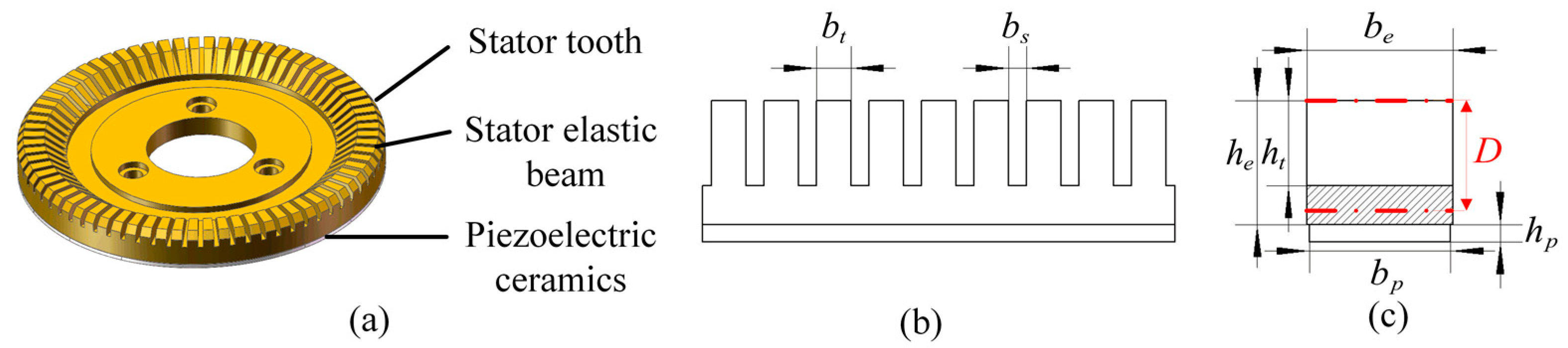
Figure 2.
A schematic diagram of the stator vibration mode and contact state: (a) schematic diagram of the stator vibration mode; (b) a schematic diagram of the stator and rotor contact state; and (c) a motion diagram of the particle point at the stator drive end.
Figure 2.
A schematic diagram of the stator vibration mode and contact state: (a) schematic diagram of the stator vibration mode; (b) a schematic diagram of the stator and rotor contact state; and (c) a motion diagram of the particle point at the stator drive end.
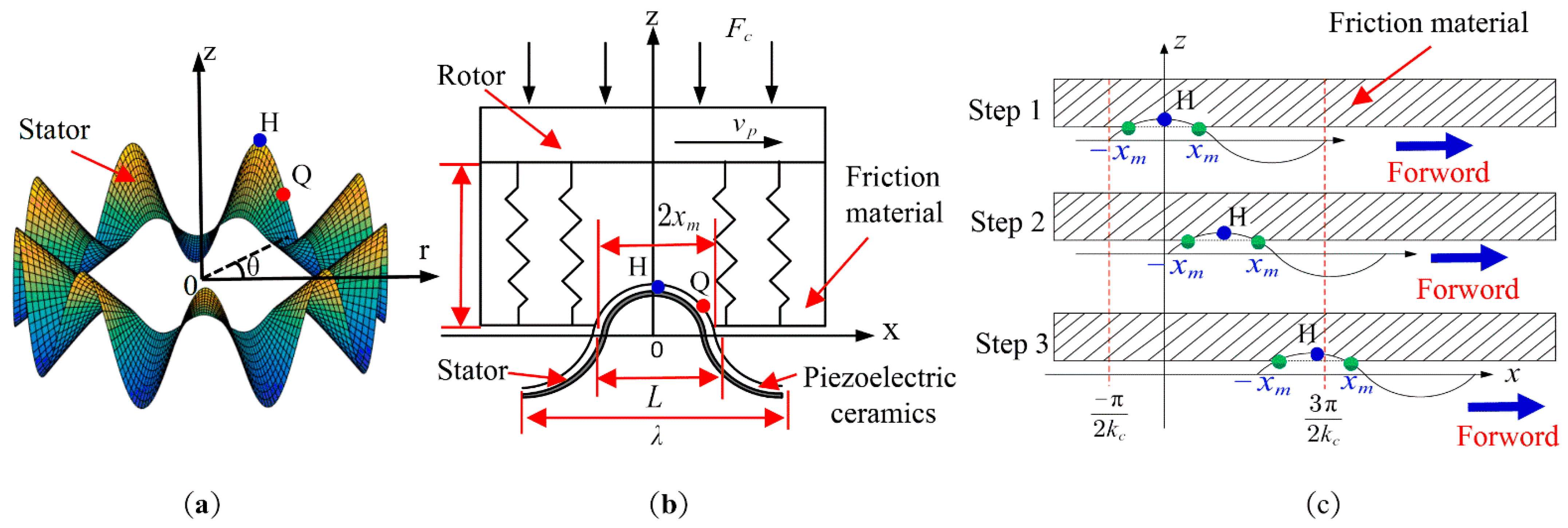
Figure 3.
A schematic diagram of the two-phase excitation response based on the superimposed pulse driving method: (a) a schematic diagram of the two-phase excitation response; and (b) a simulation diagram of the stator modal shape.
Figure 3.
A schematic diagram of the two-phase excitation response based on the superimposed pulse driving method: (a) a schematic diagram of the two-phase excitation response; and (b) a simulation diagram of the stator modal shape.
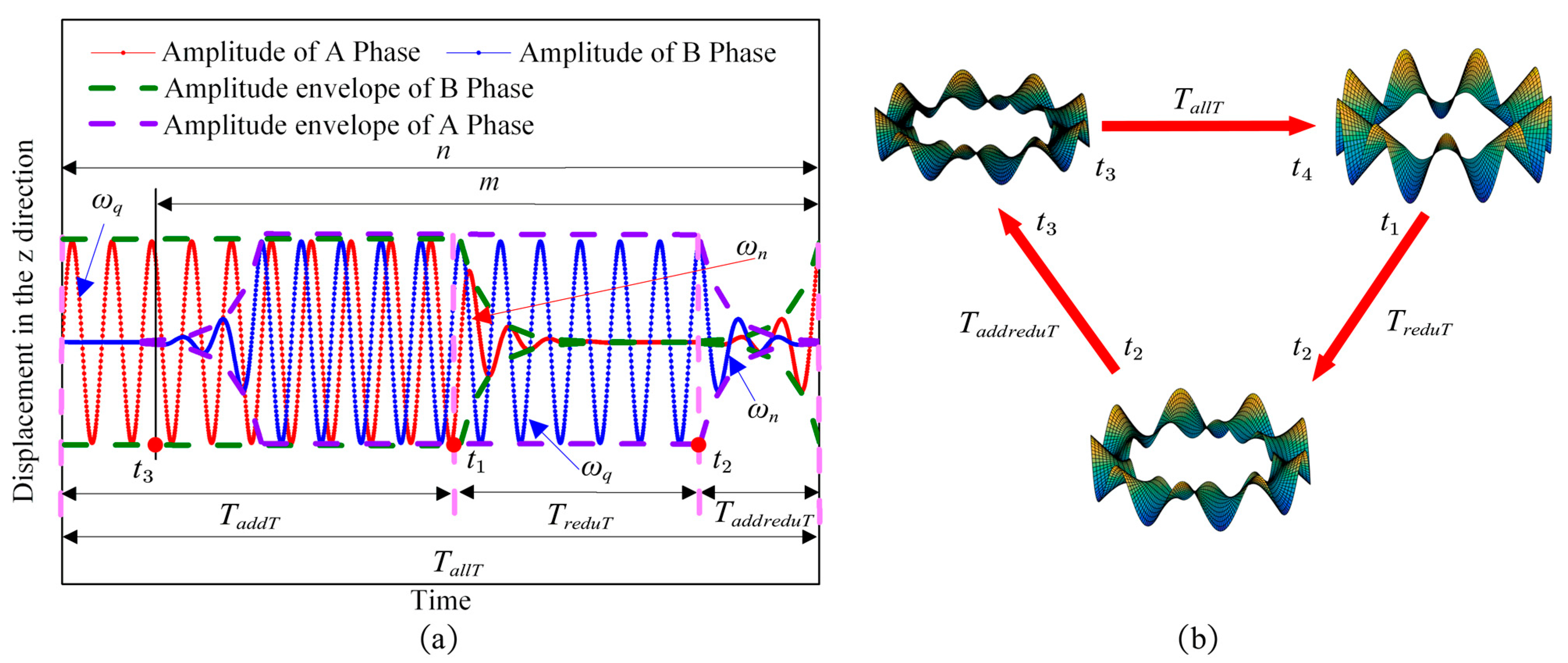
Figure 4.
Schematic diagram of the elliptical coordinate system and determinant coordinate system: (a) schematic diagram of the elliptical coordinate system; (b) schematic diagram for the determining factors of the elliptical motion direction in ; (c) schematic diagram for the determining factors of the elliptical motion direction in ; and (d) schematic diagram for the determining factors of the elliptical motion direction in .

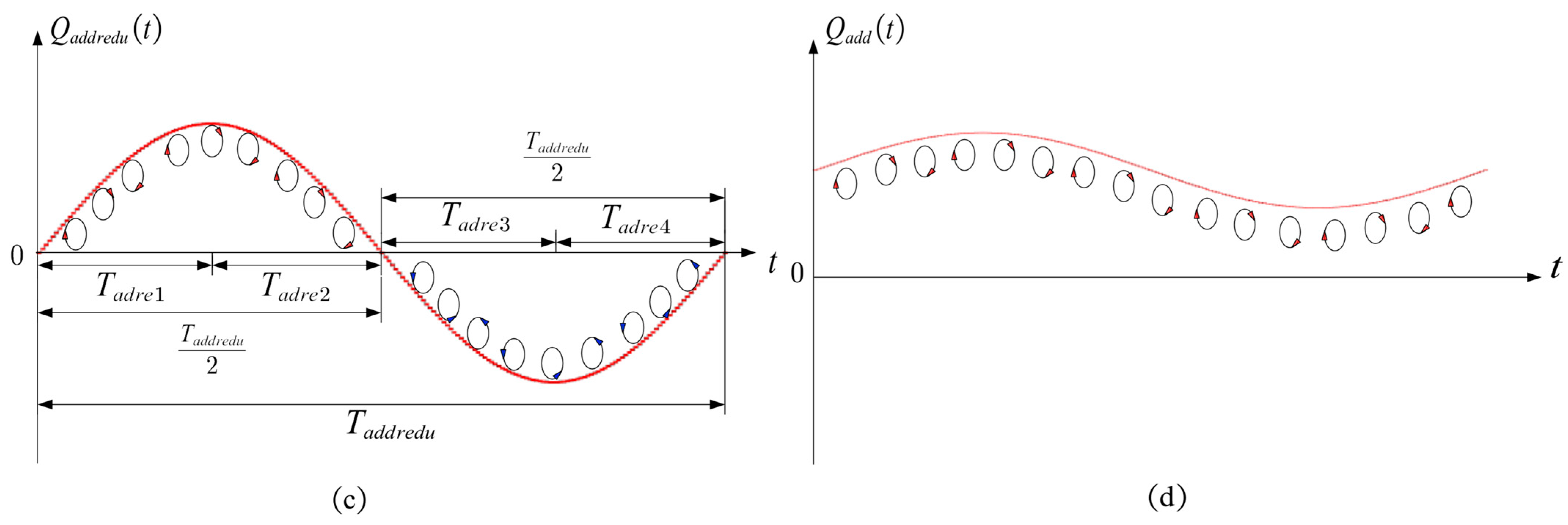
Figure 5.
Contact models of the interface between the stator and the rotor.
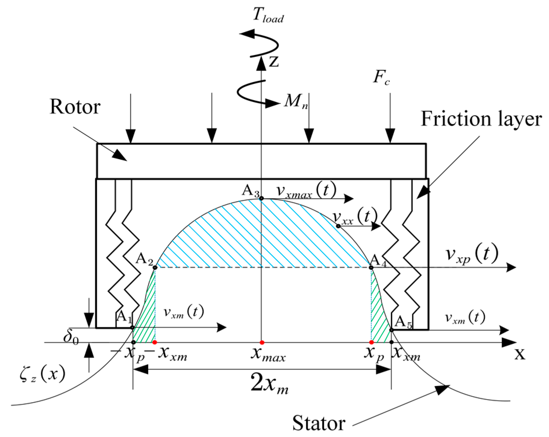
Figure 6.
Instantaneous tangential velocity of particle point Q.
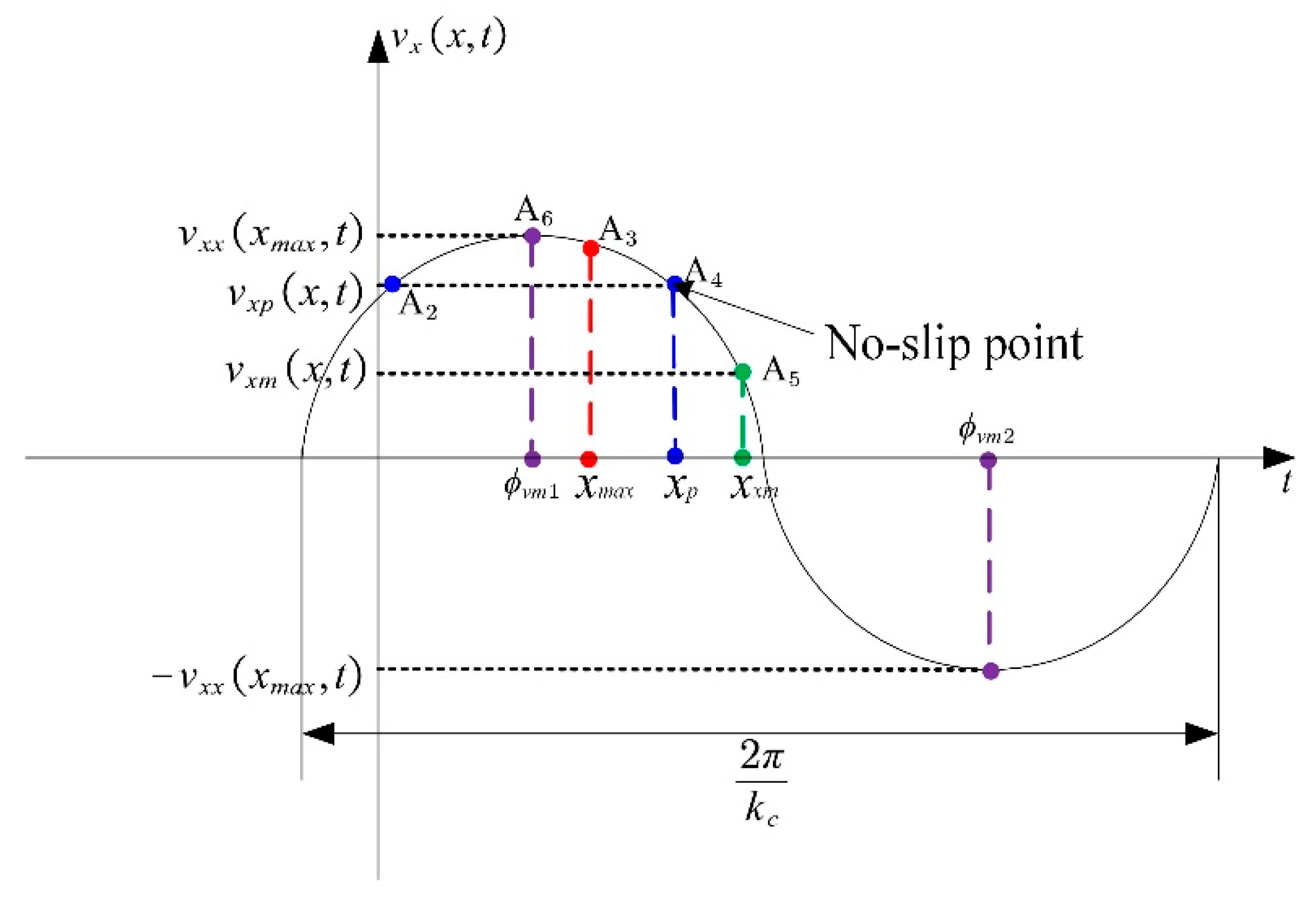
Figure 7.
Forward nonsliding point transfer model.
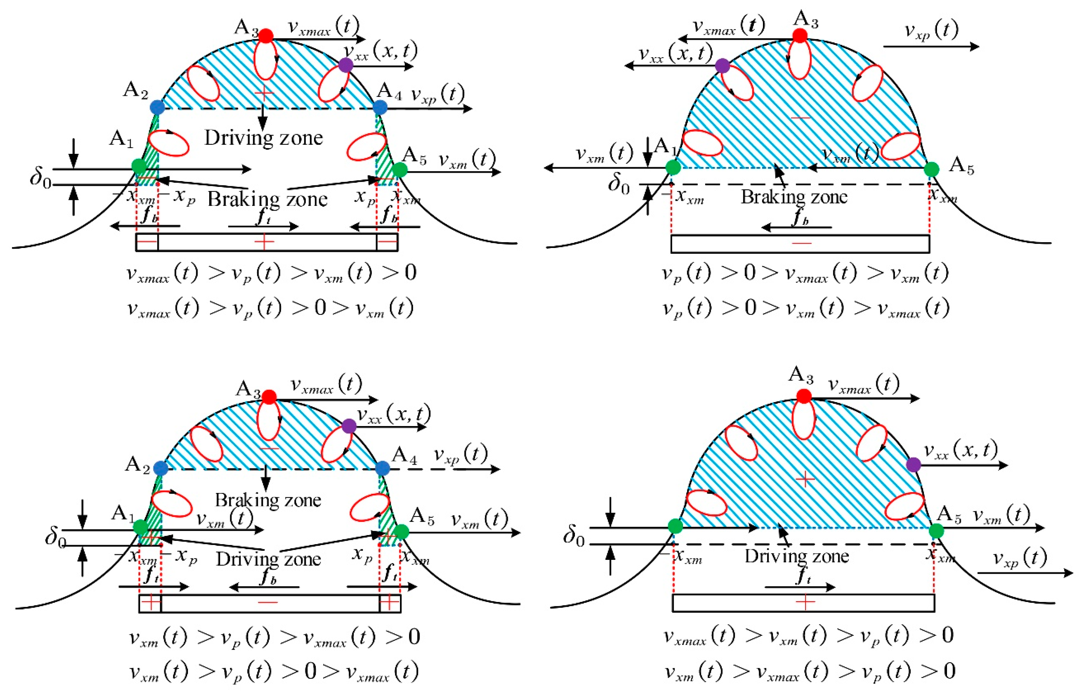
Figure 8.
Reverse sliding point transfer model.

Figure 9.
Elliptical trajectory of particle Q.

Figure 10.
Displacement variation curve of the vertical direction.
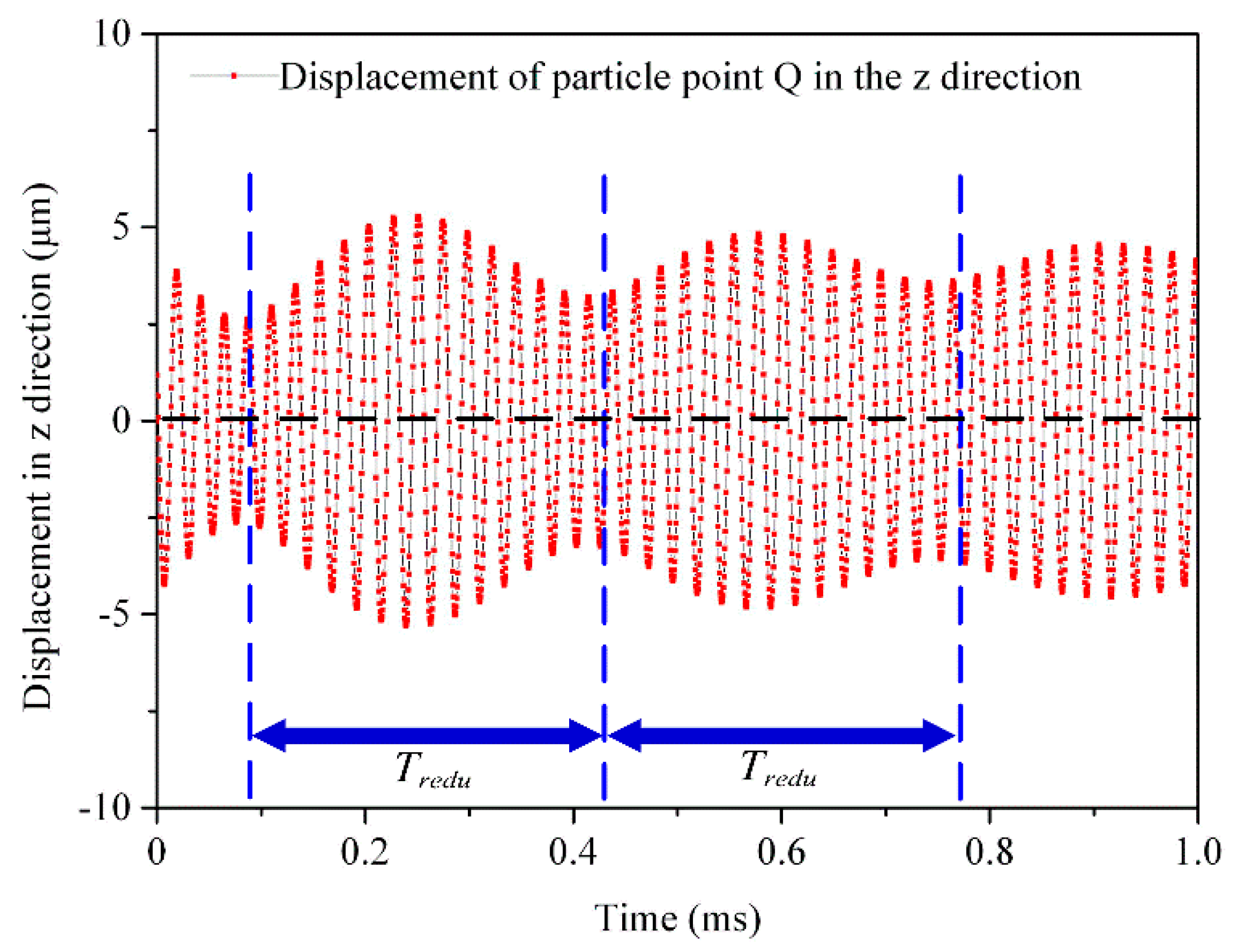
Figure 11.
Variation curve of the determining factor equation for the elliptical motion direction.
Figure 12.
Elliptical trajectory of particle Q.
Figure 13.
Displacement variation curve of the vertical direction.

Figure 14.
Variation curve determining factor equation for the elliptical motion direction.
Figure 15.
Elliptical trajectory of particle Q.

Figure 16.
Displacement variation curve for the vertical direction.

Figure 17.
Variation curve of the determining factor equation for the elliptical motion direction.
Figure 18.
Schematic diagram for the instantaneous velocity of the rotor.

Figure 19.
Schematic diagram of determining factors for the direction of the motion.

Figure 20.
The simulation curve for the determining factors of motor instantaneous speed and elliptical direction of motion with frequency difference: (a) simulation curve of motor instantaneous speed; and (b) simulation curve of determining factors for the elliptical direction of motion within one cycle of the superimposed pulse driving method.
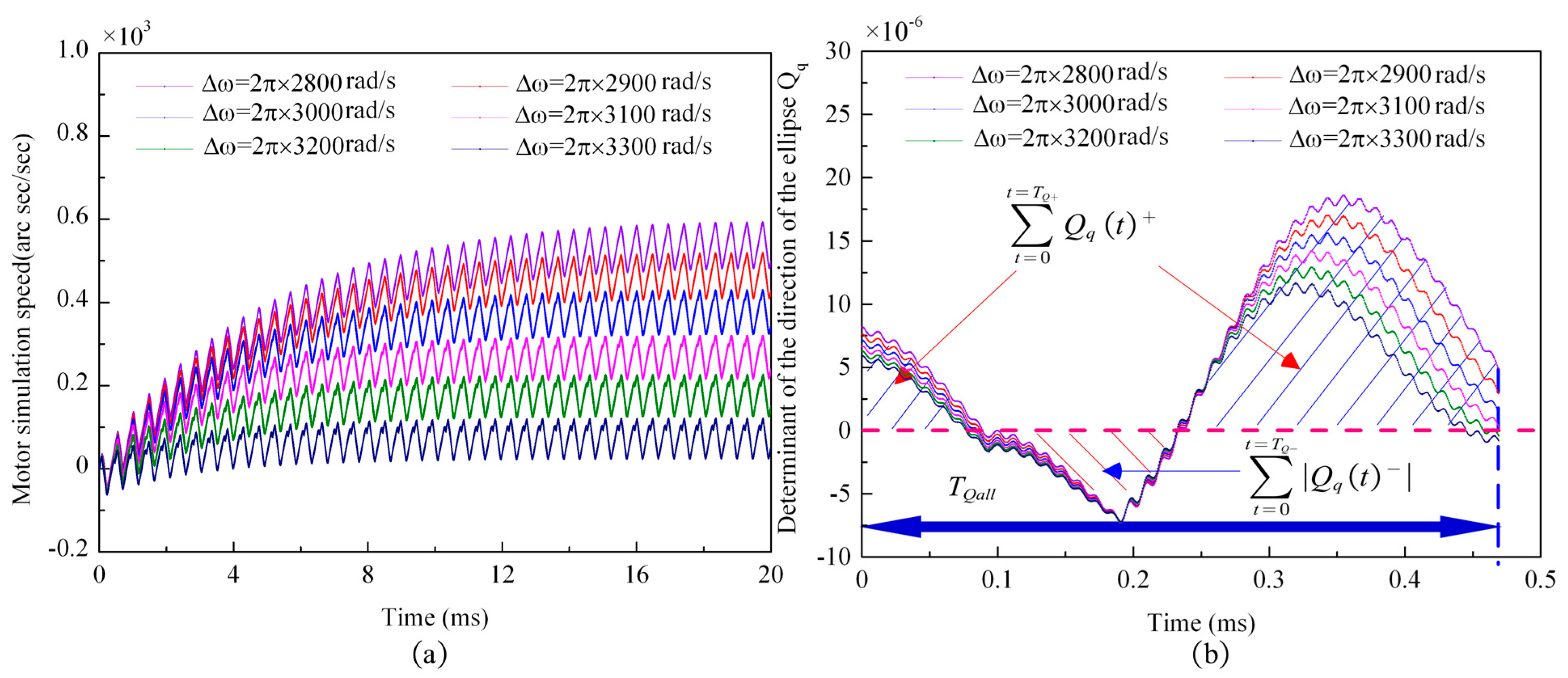
Figure 21.
Simulation diagram of characteristic variables changing with frequency difference: (a) a simulation diagram of the motor’s average speed, , and the motor’s average speed determinant, , changing with the frequency difference; and (b) a simulation diagram of the speed volatility determinant, , and the speed volatility, , changing with the frequency difference.
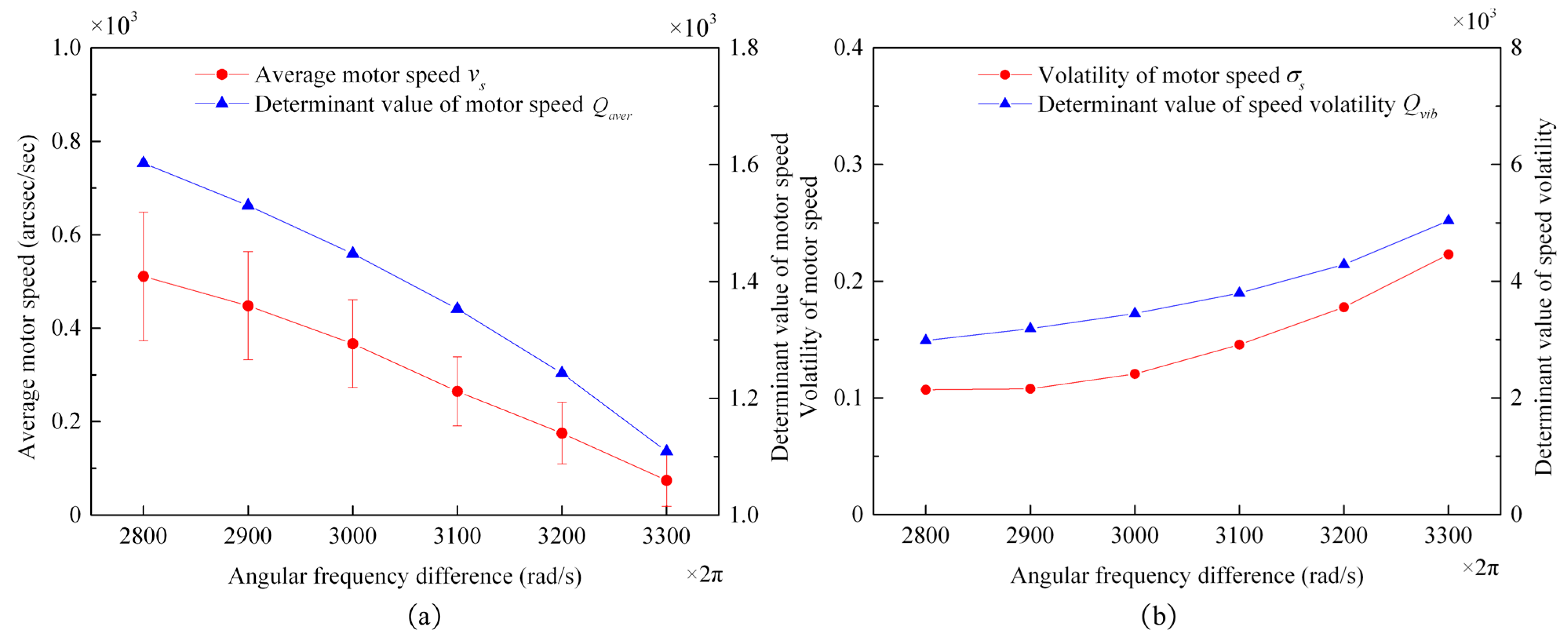
Figure 22.
Simulation diagram of the characteristic variables changing with prepressure: (a) a simulation diagram of the motor’s average speed, , and the motor’s average speed determinant, , changing with the prepressure; and (b) a simulation diagram of the speed volatility determinant, , and the speed volatility, , changing with the prepressure.
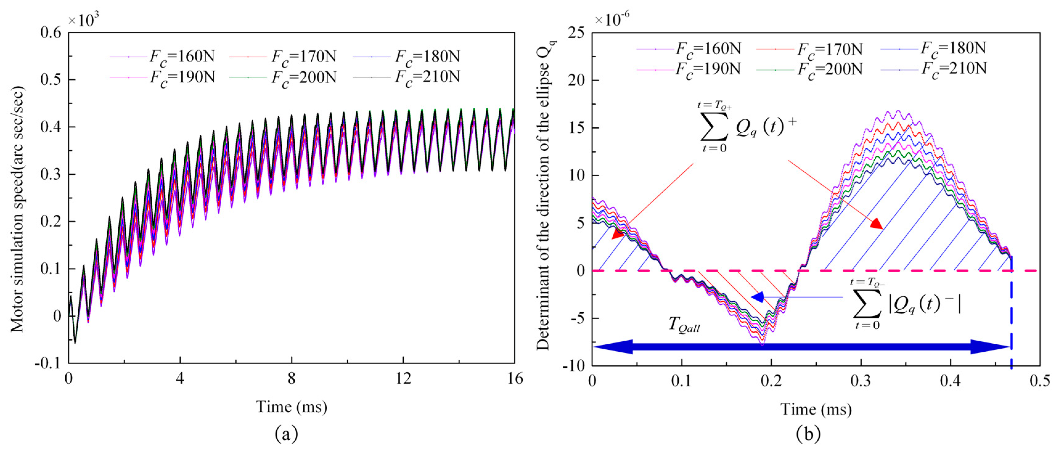
Figure 23.
Simulation diagram of the characteristic variables changing with prepressure: (a) a simulation diagram of the motor’s average speed, , and the motor’s average speed determinant, , changing with the prepressure; and (b) a simulation diagram of the speed volatility determinant, , and the speed volatility, , changing with the prepressure.
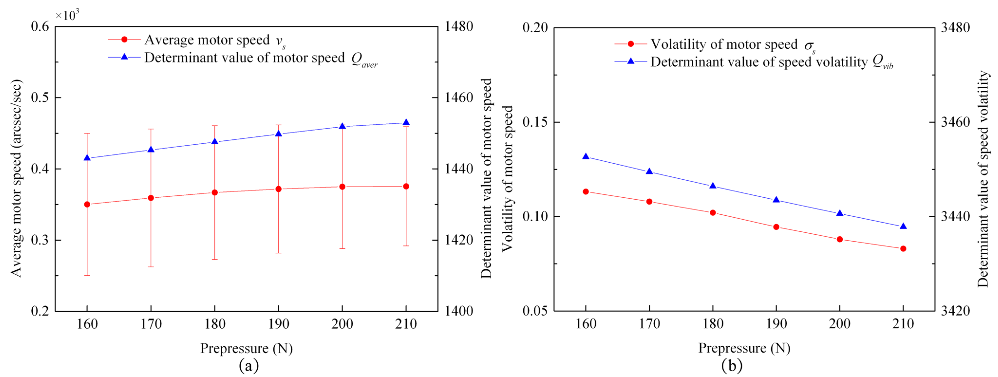
Figure 24.
Tooling diagram of stator amplitude test with prepressure.

Figure 25.
Resonance frequency measurement diagram with prepressure: (a) a resonance frequency test kit diagram with prepressure; and (b) a comparison diagram of the experimental test results and theoretical calculation results with the change in prepressure.
Figure 25.
Resonance frequency measurement diagram with prepressure: (a) a resonance frequency test kit diagram with prepressure; and (b) a comparison diagram of the experimental test results and theoretical calculation results with the change in prepressure.
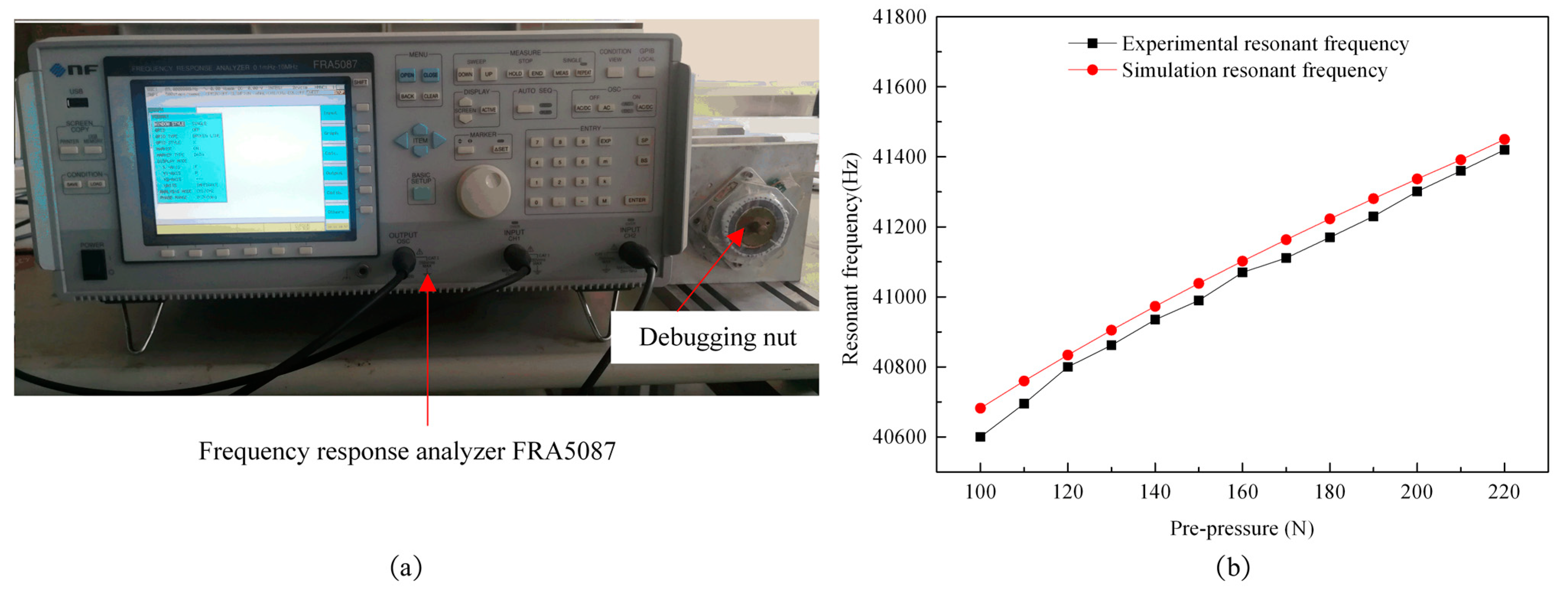
Figure 26.
A stator single-phase vibration measurement experiment diagram: (a) vibration measurement fixture diagram; and (b) velocity measurement diagram of particle M on the stator surface in the vertical direction.
Figure 26.
A stator single-phase vibration measurement experiment diagram: (a) vibration measurement fixture diagram; and (b) velocity measurement diagram of particle M on the stator surface in the vertical direction.
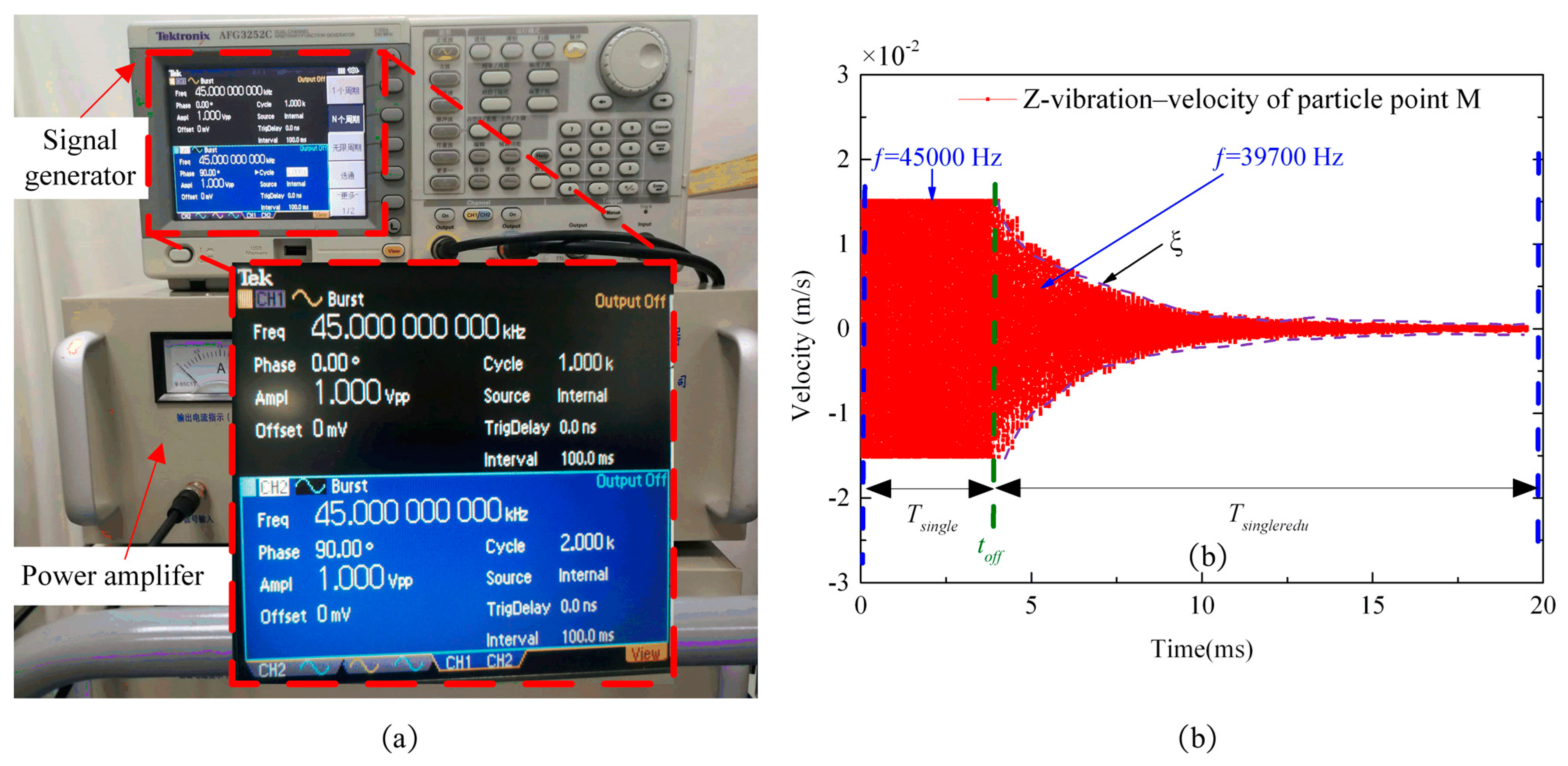
Figure 27.
Schematic diagram of the two-phase excitation response in the stator two-phase vibration measurement experiment: (a) a schematic diagram of the two-phase excitation response; and (b) a measurement diagram of the vertical velocity of particle point M on the stator surface.
Figure 27.
Schematic diagram of the two-phase excitation response in the stator two-phase vibration measurement experiment: (a) a schematic diagram of the two-phase excitation response; and (b) a measurement diagram of the vertical velocity of particle point M on the stator surface.
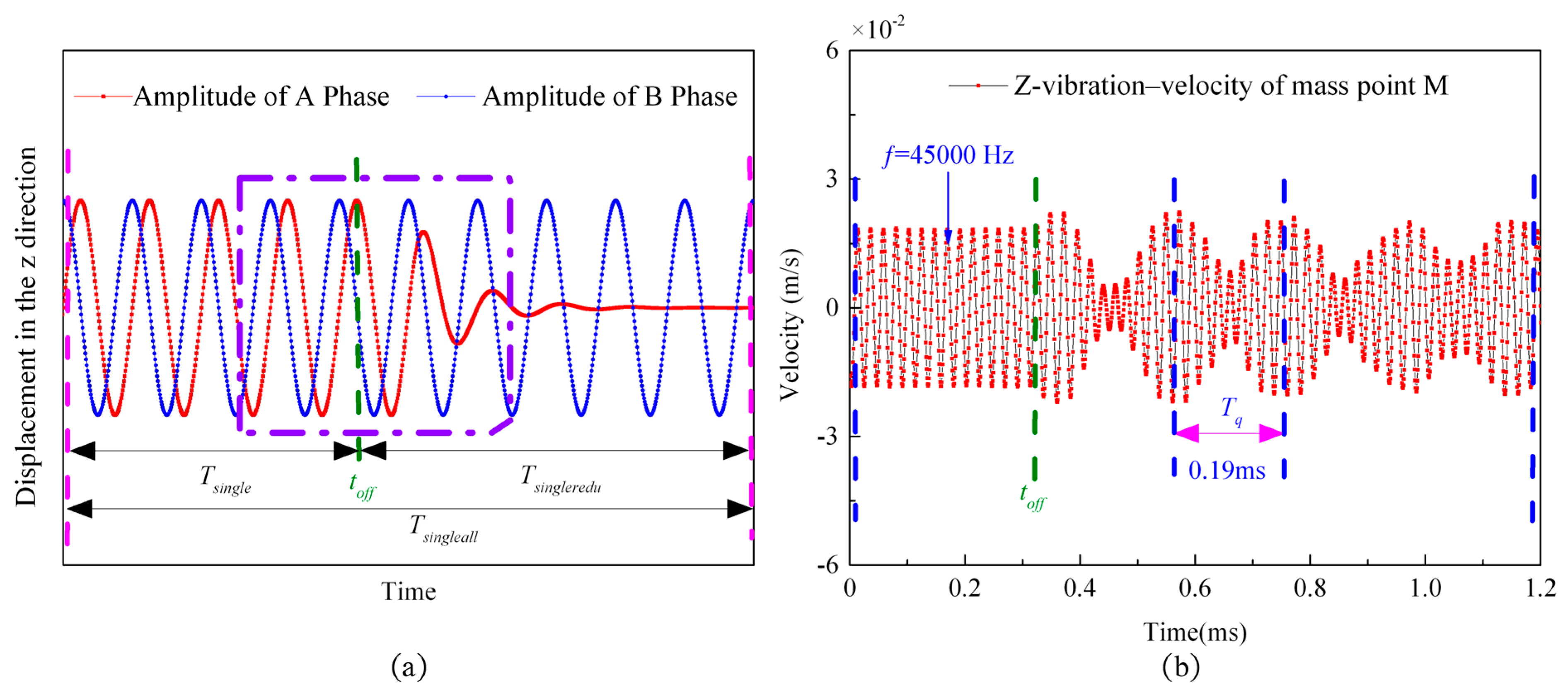
Figure 28.
Configuration of the experiment platform.
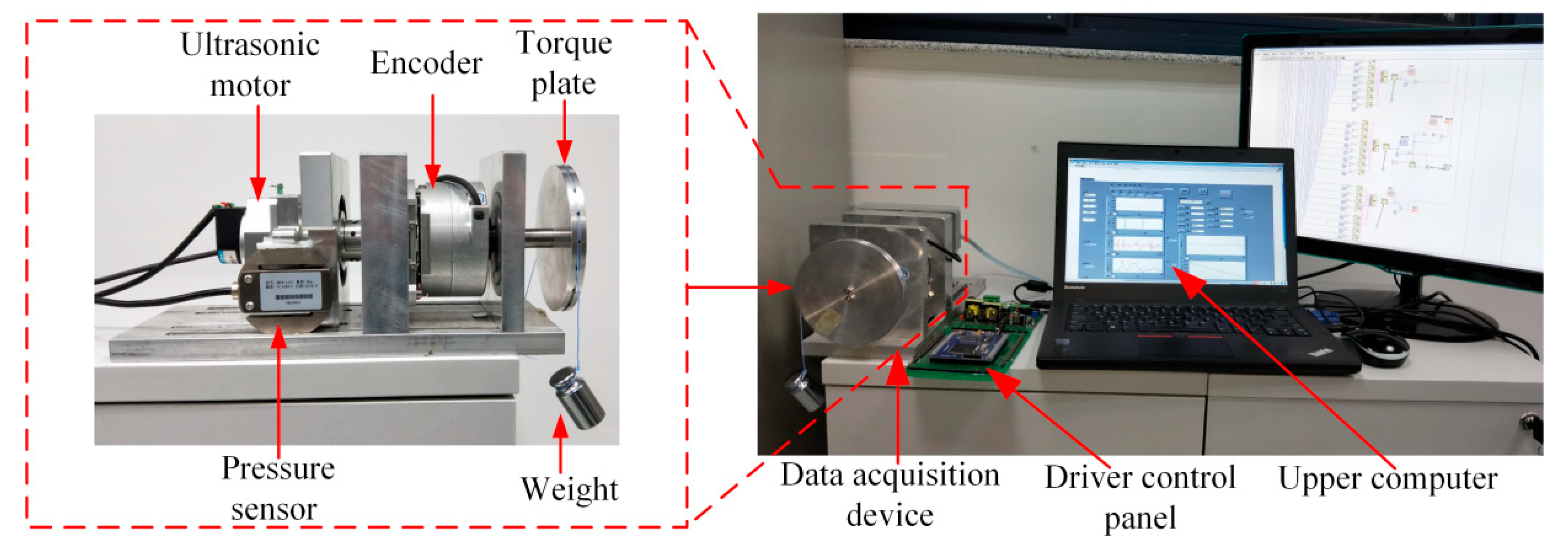
Figure 29.
Motor speed measurement diagram.

Figure 30.
An experimental diagram of the variation trend of characteristic variables with frequency difference: (a) an experimental diagram of the motor’s average speed, , and the motor’s average speed determining factor, , with frequency difference; and (b) an experimental diagram of the speed volatility, , and the speed volatility determinant, , with frequency difference.
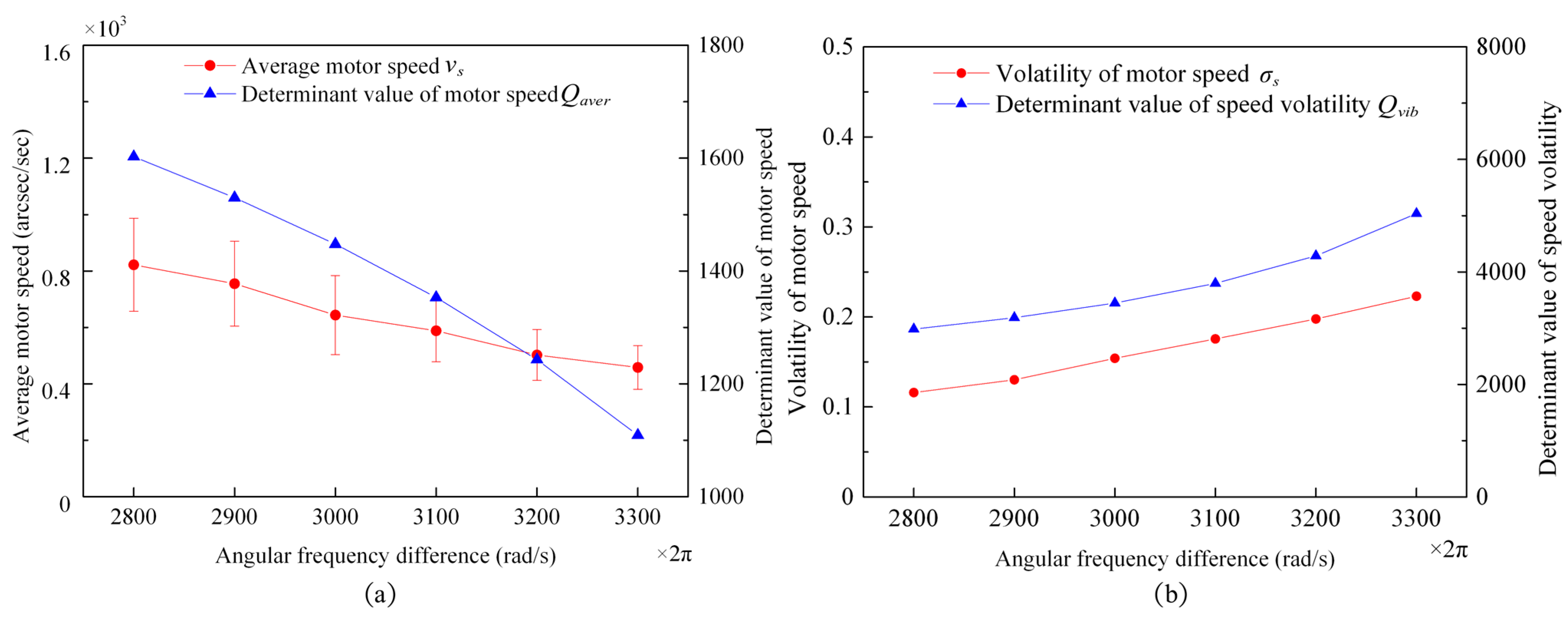
Figure 31.
An experimental diagram of the variation trend of characteristic variables with prepressure: (a) an experimental diagram of the motor’s average speed, , and the motor’s average speed determining factor, , with prepressure; and (b) an experimental diagram of the speed volatility, , and the speed volatility determinant, , with prepressure.
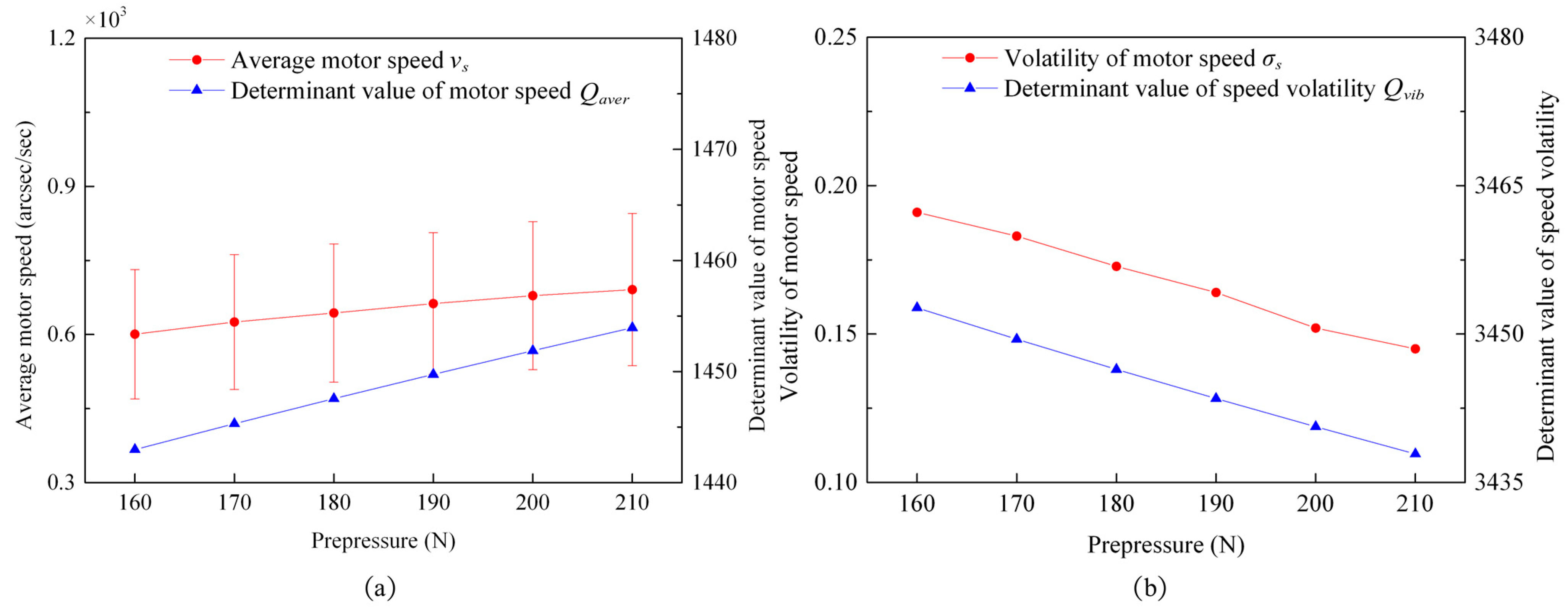
Figure 32.
Experimental diagram of the trend in characteristic variables changing with multiple control variables: (a) an experimental diagram of the motor’s average speed, , and the motor’s average speed determining factor, ; and (b) an experimental diagram of the tendency of the speed volatility, , and the speed volatility determinant, .


Table 1.
The simulation parameters of TRUM60.
| Parameter | Description | Numerical Value (Unite) |
|---|---|---|
| Stator radius | ||
| Number of stator teeth | 72 | |
| Stator perimeter | ||
| Stator slot width | ||
| Stator elastic beam width | ||
| Friction material width | ||
| Stator elastic beam thickness | ||
| Stator teeth thickness | ||
| Piezoelectric material thickness | ||
| Friction material thickness | ||
| Stator elastic beam density | ||
| Piezoelectric material density | ||
| Friction material density | ||
| Stator elastic beam Young’s modulus | ||
| Piezoelectric material Young’s modulus | ||
| Friction material Young’s modulus | ||
| Stator elastic beam shear modulus | ||
| Piezoelectric material shear modulus | ||
| Stator elastic beam Poisson’s ratio | 0.33 | |
| Piezoelectric material Poisson’s ratio | 0.31 | |
| Friction material Poisson’s ratio | 0.3 | |
| Damping ratio | 0.006 | |
| Height-width ratio of the beam section | 0.9 | |
| Piezoelectric voltage | ||
| Mortor load | 0.3 (N·m) | |
| Moment of inertia of the rotor | 4.5 × 10⁻⁶ | |
| κ | Shear correction coefficient | 0.9 |
Table 2.
Stator amplitude test results under different prepressures.
| (N) | 100 | 120 | 140 | 160 | 180 | 200 | 220 |
| (μm) | 8.3 | 7.3 | 6.6 | 6.0 | 5.5 | 5.2 | 4.8 |
Table 3.
Parameter setting table.
| Parameters | Value |
|---|---|
| 14 | |
| 20 | |
| 0.3 (N·m) | |
| 180 (N) |
Table 4.
Result analysis table.
| Parameters | Value |
|---|---|
| 633 (acr s) | |
| 400 (arc s/s) | |
| 1447.5 | |
| 17.3% | |
| 3446.4 |
Table 5.
Multicontrol variable set values table.
| Experimental Test Number | 1 | 2 | 3 | 4 | 5 | 6 |
|---|---|---|---|---|---|---|
| (N) | 180 | 170 | 160 | 190 | 200 | 210 |
| (rad/s) | 3300 | 3100 | 3000 | 2800 | 2900 | 3200 |
Publisher’s Note: MDPI stays neutral with regard to jurisdictional claims in published maps and institutional affiliations. |
© 2021 by the authors. Licensee MDPI, Basel, Switzerland. This article is an open access article distributed under the terms and conditions of the Creative Commons Attribution (CC BY) license (https://creativecommons.org/licenses/by/4.0/).
Share and Cite
MDPI and ACS Style
Zeng, W.; Pan, S.; Chen, L.; Ren, W.; Hu, X. Research on Low-Speed Driving Model of Ultrasonic Motor Based on Beat Traveling Wave Theory. Actuators 2021, 10, 304. https://doi.org/10.3390/act10110304
AMA Style
Zeng W, Pan S, Chen L, Ren W, Hu X. Research on Low-Speed Driving Model of Ultrasonic Motor Based on Beat Traveling Wave Theory. Actuators. 2021; 10(11):304. https://doi.org/10.3390/act10110304
Chicago/Turabian StyleZeng, Weijun, Song Pan, Lei Chen, Weihao Ren, and Xiaobin Hu. 2021. "Research on Low-Speed Driving Model of Ultrasonic Motor Based on Beat Traveling Wave Theory" Actuators 10, no. 11: 304. https://doi.org/10.3390/act10110304
Note that from the first issue of 2016, this journal uses article numbers instead of page numbers. See further details here.