Article

Position Control of the Dielectric Elastomer Actuator Based on Fractional Derivatives in Modelling and Control

Faculty of Mechanical Engineering, University of Maribor, 2000 Maribor, Slovenia
*
Author to whom correspondence should be addressed.
Actuators 2021, 10(1), 18; https://doi.org/10.3390/act10010018
Submission received: 28 December 2020 / Revised: 11 January 2021 / Accepted: 18 January 2021 / Published: 19 January 2021
(This article belongs to the Special Issue Artificial Muscles and Soft Actuation)

Abstract

:
Successful control of a dielectric elastomer actuator (DEA) can be a challenging task, especially if no overshoot is desired. The work presents the first use of the P I λ D μ control for a dielectric elastomer actuator to eliminate the overshoot. The mathematical model of the dielectric elastomer was established using the fractional Kelvin-Voigt model. Step responses are first tested in the Laplace domain, which gave the most satisfactory results. However, they did not represent the real model. It cannot have negative force acting on the dielectric elastomer actuator. Simulations in Matlab/Simulink were performed to obtain more realistic responses, where output of the P I λ D μ controller was limited. Initial parameters for a PID control were obtained by the Wang–Juang–Chan algorithm for the first order plus death time function approximation to the step response of the model, and reused as the basis for the P I λ D μ actuator control. A quasi-anti-windup method was introduced to the final control algorithm. Step responses of the PID and the P I λ D μ in different domains were verified by simulation and validated by experiments. Experiments proved that the fractional calculus P I λ D μ step responses exceeded performance of the basic PID controller for DEA in terms of response time, settling time, and overshoot elimination.

1. Introduction

Soft actuators are actuators whose performance tries to mimic the behavior of a biological muscle. A biological muscle performs only two simple motions: contraction and relaxation. Even though this movement seems very simple, the reality is quite the opposite. The basic structure of a biological muscle is a bundle of muscle fibers. Muscle fibers are a compound of myofibrils, of which the basics are sarcomeres. A sarcomere has two parts: myosin filaments and actin filaments. They interact with each other with the help of C a 2 + ions. The presence of C a 2 + ions contracts the muscle fiber by δ L , whereby the duration of the contraction depends on the amount of these ions [1]. Contraction of the muscle generates F force; the product of contraction and force is A = δ L   ·   F . If A is measured over time, one can obtain power P = F   ·   δ L / δ t generated by the contraction of a muscle.
Regarding the activation principle, soft actuators that are most like biological muscles are ionic electroactive polymers [2,3]. They deform their principal shape when there is an internal difference in the ionic state. Even though the principle is similar, its deformation differs from biological muscles. They usually exhibit bending movement with a very slow deformation rate. Activation energy to change ionic state is applied by electrical energy. It is a reverse process, but it has a slow recovery rate.
On the other hand, there is another group of soft actuators called dielectric elastomer actuators, also known as DEAs. Their activation energy is also electricity with 1000 times higher potential then in ionic actuators. The principle of the activation of the structure differs from ionic actuators. DEA has a similar structure as a parallel plated capacitor. It has upper and lower conductive electrodes with elastomer used as the dielectric. Elastomer is considered incompressible. Its Poisson number is 0.5. Only direct current can be applied on a DEA. When DC voltage is applied, attractive force is generated between the positive and negative potentials. This is also called the Maxwell stress. Figure 1 shows the basic structure and principle of activation of a planar DEA. When DC voltage is applied, the elastomer dimensions change from l 1 l 1 , l 2 l 2 , and l 3 l 3 according to Figure 1. The ratio of change in each direction can be described as δ 1 = l 1 / l 1 , δ 2 = l 2 / l 2 , and δ 3 = l 3 / l 3 , respectively. Since elastomer is incompressible, the following applies: 1 = δ 1 δ 2 δ 3 .
The basic principles of DEAs’ movement are not the same as for biological muscles, but, in comparison with ionic actuators, they move much faster and exhibit larger movements. Under applied voltage they can also hold the tension or position. As such, they can be used as soft actuators with similar behavior as biological muscles.
The introduction of fractional calculus dates back to the 17th century, where Leibniz addressed a letter to L’Hopital asking him about the existence of a half derivative [4]. This date is marked as the beginning of fractional calculus. Fractional calculus defines integrals and derivatives with non-integer orders, so the name might be a bit confusing, but since then, this term has been generally accepted. Two centuries later the proper definition was developed, with the works of Riemann et al. [5].
Fractional calculus can be used in different areas. Lately it is being used in describing the bursting of the two pancreatic β-cells working in synchronization. With the help of changing only fractional orders, they are able to model different bursting activities of insulin [6]. Studying biological conditions with memory characteristics that can be defined with the fractional calculus is another interesting area of use [7]. Readers interested in areas where fractional calculus is expanding should refer to the work of Sun et al. [8]. Among others, the main areas of research with fractional calculus are in physics, control, signal and image processing, mechanics and dynamic systems, biology, environmental science, materials, viscoelasticity, and economics [8]. Fractional calculus is also being used to describe fractional order chaotic systems, systems that are very sensitive to initial conditions [9]. One such interesting area for using fractional calculus is rheology, part of which is viscoelasticity. The behavior of viscoelastic materials can be simulated using fractional calculus in rheological models, where basic rheological models can be converted into fractional ones [10]. It can also be used in control theory to convert a classical PID controller into a fractional one [5,11,12]. Expressed as P I λ D μ , the fractional controller has five tuning parameters, which enables a wider fitting range for fine tuning.
Since most dielectrics used in DEA applications perform viscoelastic behavior, it is challenging to achieve satisfactory position control without overshoot. Babič et al. [13] used a basic Kelvin-Voigt model for material parametrization and self-tuning PID control. They got the first parameters for PID from the Ziegler–Nichols open-loop method. An experiment was conducted with DEA attached to a servo linear motor that maintained a constant force for pre-stretching. They were able to generate displacements up to 2 mm. Position control had 10–20% of overshoot and 0% of stationary error.
In the work of Sarban et al. [14], they used a Kelvin-Voigt model with three springs in series, where two springs had dampers in parallel connections for material parametrization of an adaptive vibrational isolator in cylindrical form. They used feedforward control, a method based on knowing the mechanical behavior of the plant. The feedforward adaptive control approach was used to predict the mechanical behavior of the isolator. They achieved active vibrational isolation but had no measured step responses.
The Gent model is also commonly used for the parametrization of viscoelastic materials, and it has one spring and a pair of spring dampers in parallel connection. It was used in the work of Li et al. [15] for DEA parametrization. They used PID control on the proposed model on a sine wave reference signal. They were able to capture amplitude and frequency, but with a phase shift of 90°.
In the work of Ngujen et al. [16], they used the Mooney–Rivlin model for the material parametrization of cylindrically configured DEA. They used a PWM-PID control that did not eliminate overshoot and still performed small oscillation around the reference point.
In the work of Mustaza et al. [17], they used a modified Voigt model for the material parametrization of a DEA compound of three equally spaced cylinders disposed at 120° in a symmetrical radial configuration. The modified Voigt model had been already introduced by Yeoh [18]. Displacement control was implemented with the help of model-based control. The performance of the control depended on the accuracy of the material parametrization. Experiments show that although control is possible, overshoot and static error are not eliminated.
A worm-like soft actuator was created as well as a controller in the work of Cao et al. [19]. For material parametrization they used a multi-layer Kelvin-Voigt model. They used feedforward plus feedback control schemes. They used a PI control in the feedback loop. Its parameters were gained with the help of the Nichols–Ziegler method. Simulations were tested in MATLAB/Simulink, where step responses were given without overshoot or static errors. Once tested on a real model, the performance of the proposed control algorithm showed poor performance regarding overshoot and static error.
In the work of Rizzello et al. [20,21], DEA in the shape of an annular membrane was used for position control. It was pre-stretched on the disc, so there was no need for additional load. However, a spring and an additional load were attached to the actuator. The model was derived with the help of Helmholtz free energy and a nonlinear version of a standard linear solid model. Position control was performed with PID, with the linearization of the model with PID, and with a robust H control algorithm. Although PID control gave satisfactory results, overshoot was not eliminated. On the other hand, linearized PID and H control gave excellent performance with little to no overshoot.
As can be seen, it is quite challenging to eliminate overshoot when dealing with position control on viscoelastic materials.
The use of fractional calculus in mathematical modeling and position control of the DEA is presented for the first time to improve the step response of the DEA and to eliminate the overshoot. The planar structure of DEA is used where pre-stretch is maintained with the help of appropriate weight. Since the performance of the PID control did not give satisfactory results, the control was upgraded to fractional control with the help of the P I λ D μ . The step response of the model was compared to the step response of the first order plus death time (FOPDT) function. The parameters for the PID controller were obtained with the help of FOPDT and the Wang–Juang–Chan algorithm. These parameters and λ = μ = 0.5 are starting parameters for a P I λ D μ controller. Nevertheless, the FOMCON toolbox was used in the search for the optimal parameters for the P I λ D μ controller [22]. With its help, different starting parameters were chosen to find the optimal parameters. The step responses of optimal parameters were tested in Laplace, time, and discrete domains, where responses were, surprisingly, not the same. Consequently, all optimized parameters needed to be validated with a real experiment. For the implementation of P I λ D μ to a real controller, its fractional order of integration and derivation needs to be approximated with an Oustaloup filter. The new transfer function of P I λ D μ with fractional orders approximated can be transformed into a discrete domain and implemented into the microcontroller. Implementing the standard PID Simulink block on a microcontroller provides an anti-windup method for limiting the output of the integrator. However, the possibility of integral windup is not eliminated by implementing P I λ D μ in the form of an approximated discrete transfer function. Consequently, a quasi-anti-windup method was developed and implemented on the microcontroller. Real experiments showed the advantages of using P I λ D μ over a PID controller regarding response time, settling time, and overshoot.
In the Materials and Methods section, a summary is given of the fractional calculus applied to the Kelvin-Voigt model and on parameter identification. Some basics are also presented for the use of fractional calculus in control theory. A Laplace transformation was employed to transform the fractional Kelvin-Voigt model into the s-domain. The step response was analyzed and compared with the step response of the first order plus death time (FOPDT) function. After the parameters of the FOPDT function were identified, the Wang–Juang–Chan algorithm was introduced to identify parameters of the PID controller [23]. The identified parameters represented the starting points for parameter identification of the P I λ D μ controller. The optimization of the P I λ D μ controller was explained using the FOMCON toolbox in Matlab [22]. The P I λ D μ controller needed to be transformed into the Laplace and discrete domain from the time domain. Also presented is the implementation of the P I λ D μ controller to a microcomputer. A quasi-anti-windup method was introduced to limit windup output of the approximated controller in the real experiment.
The simulation results were validated by experiments and deviations in different domain models are presented in the Results section.
The Discussion section highlights conclusions and outlines proposals for future work.

2. Materials and Methods

2.1. Using Fractional Calculus in Rheology and Control Theory

To apply a dielectric elastomer actuator (DEA) as a controlled soft actuator one needs to develop the governing equations of the system. The DEA uses the elastomer as the main platform on which conductive electrodes are applied. The elastomer VHB 4910 from the company 3M was used in this specific case [24]. The planar structure of the DEA was used as shown in Figure 1. The elastomer was cut to the initial non stretched dimensions of (50 × 49 × 1) mm according to the coordinate system used in Figure 1. After inserting the elastomer into the gripping jaws the dimensions between the jaws was (10 × 49 × 1) mm. Conductive paste from Bare Conductive [25] was applied to the stretched elastomer, where the dimensions changed to (60 × 49 × 0.16) mm. Since high voltage can spark over the edge, creating a short circuit, the active surface of the DEA was reduced to (60 × 40) mm. Figure 2 shows the planar configuration of the stretched elastomer and active surface of the DEA, as well as the applied coordinate system. When DC voltage is applied, the elastomer expands in the longitudinal or x direction. However, small movement is also seen in the y direction, which represents the loss of energy in the system.

2.1.1. Fractional Calculus in Rheology

Dynamic analysis of the used elastomer revealed viscoelastic behavior, which means that the elastomer performed with both elastic and viscous behavior. According to [10,26,27], one can model material behavior with fractional calculus and rheology. Using the Kelvin-Voigt model and fractional calculus, one can modify the basic Kelvin-Voigt model to a fractional Kelvin-Voigt model, which consists of two parts: a spring and a springpot. The springpot is an element that is a combination of a spring and a dashpot. Its characteristic is determined with the springpot constant and the derivative order
F ( t ) = k x ( t ) + c d α x ( t ) d t α
which is its main advantage over the basic Kelvin-Voigt model [5,10,27]. In Equation (1) the Grünwald–Letnikov definition of fractional derivative is used
a D t p f ( t ) = lim h 0 h p r = 0 n ( 1 ) r ( p r ) f ( t r h ) .
The Grünwald–Letnikov definition is chosen since it can easily handle fractional derivation (p) and integration (−p), and it is also suitable for the numerical calculation of fractional derivatives and does not lead to difficulties when applying it to real-world problems [5,28].
If the derivative order of a springpot equals 1, the element represents a dashpot; if the derivative order equals 0, the element represents a spring. With fractional calculus the derivative order is no longer limited to integers and can be any real number between 0 and 1.

2.1.2. Fractional Calculus in Control Theory

To show that the fractional Kelvin-Voigt model is stable it must be transformed into the Laplace domain and written in the form of commensurate order.
A Laplace transform in fractional calculus transforms fractional derivation into fractional multiplication and fractional integration into fractional division. The following equation,
{ d 0.47 f ( t ) d t 0.47 } = s 0.47 { f ( t ) }
represents the Laplace transform of a fractional derivative with zero initial conditions.
The following equation,
x ( s ) F ( s ) = 1 c s α + k
represents the transfer function of the fractional Kelvin-Voigt model. The dynamic characteristics of the elastomer VHB 4910 were identified in our previous work [29,30], where the parameters were described in the relationship of δ ε and can be used for any specific dimensions. The constants for the fractional Kelvin-Voigt model were calculated for the specified DEA according to
E = σ ε = F · L A · Δ l = k · L A k = E · L A
and
σ = η · d α ε d t α η = σ d α ε d t α = F A d α ( Δ l L ) d t α = F A 1 L d α ( Δ l ) d t α = c · L A c = η · L A .
In Equations (5) and (6), E = 1.06106   N / m m 2 , η = 0.086904   N s / m m 2 , and L = 60   m m and is the extended length in the x direction, and A = 49 × 0.16 m m 2 and is the cross-section of the elastomer.
After recalculation, the parameters were k = 0.138645   N / m m , c = 0.086904   N s / m m , and α = 0.47 , where α is the same as in the δ ε relationship. To transform it into commensurate order parameter α needs to be written in the form of α = 47 / 100 and α = β × 47 , where β = 1 / 100 [31]. If complex variable s β = σ , one can form the commensurate order transfer function of the fractional Kelvin-Voigt model:
x ( σ ) F ( σ ) = 1 c σ 47 + k
Since the order of the transfer function changed, the stability criterion also changes from
| arg ( T F ( s ) ) | > π 2
to
| arg ( T F ( σ ) ) | > β π 2 .
As can be seen in Figure 3, all poles of the commensurate order transfer function of the fractional Kelvin-Voigt model satisfied the stability criterion in Equation (9), which shows that the fractional order Kelvin-Voigt model is mathematically stable.
The equation of motion expressed with the fractional Kelvin-Voigt model is given as
F ( t ) = m x ¨ ( t ) + c d α x ( t ) d t α + k x ( t )
where m = 0.0001 kg and represents the mass of the elastomer.
Using the Laplace transform on Equation (10) one obtains the following equation:
x ( s ) F ( s ) = 1 m s 2 + c s α + k
while using the fractional derivative plant model, a logical conclusion was to use fractional PID control, which is written in the form of P I λ D μ , since more adjustable parameters are available for the fine tuning of the controller. The fractional P I λ D μ has the same parameters for gains as the basic PID, except that it has two additional parameters: derivation and integration order. Since fractional calculus is used, orders are limited to real numbers between 0 and 1. It should be noted that derivation and integration are reciprocal operations. According to the Grünwald–Letnikov definition of fractional calculus, positive order describes derivation, whereas negative order describes integration. In the case of the P I λ D μ , in the control theory it is commonly known that the integral part should be negative, even though, in most literature, it is positive.
When using fractional calculus in the plant model as well as for P I λ D μ control, one can expect different slopes in the Bode diagram. Fractional derivatives impose a phase shift of α π / 2 , where α is the derivation order. It also changes the slope to 20 α   d B / d e c . Figure 4 shows Bode diagrams for the fractional ( k = 0.138645   N / m m , c = 0.086904   N s / m m , and α = 0.47 ) and the basic Kelvin-Voigt model ( k = 0.138645   N / m m and c = 0.086904   N s / m m ). It can be seen how the slope of the fractional Kelvin-Voigt changes. To create Bode plots it is recommended to use the FOTF Matlab Toolbox [32] or the FOMCON Toolbox [22].
The next step in identifying parameters for the P I λ D μ controller was to compare the step responses of the plant model with the FOPDT function. Equation (12) shows the FOPDT function and its parameters.
G p ( s ) = k e L s T s + 1
k process   gain L process   time   delay   [ s ] T process   time   constant   [ s ]
Comparing the step responses of both functions, one can obtain the parameters of FOPDT as k = 5.6652 , L = 0.0055   s , and T = 0.7891   s . Using the Wang–Juang–Chan algorithm [23] for PID parameters identification, the following parameters were obtained: k p = 7.179 , k i = 5.665 , and k d = 0.03107 . After the parameters of the PID controller were obtained, the parameters of the P I λ D μ gains were taken from the PID, and derivative and integral orders were chosen to be both at 0.5 [33,34]. Figure 5 shows the step responses of the plant model with the PID and the P I λ D μ controller in the Laplace domain. Both controllers gave fast responses. The PID controller produced no steady-state error, whereas the P I λ D μ produced a small steady-state error of about 0.5% of the desired value, which makes sense since only half of the integrator was used.

2.2. Optimization of Parameters for the P I λ D μ Controller by the Use of the FOMCON Toolbox in Matlab and Implementation of the P I λ D μ Controller on a Microprocessor

Optimization of Parameters for the P I λ D μ Controller

The initial parameters for gains of the P I λ D μ controller were calculated with the Wang–Juang–Chan algorithm, whereas derivation and integration orders were chosen freely. Optimization of P I λ D μ parameters can be performed according to the work of Tepljakov [22,33], who developed the FOMCON toolbox, which stands for Fractional Order Modeling and Control. Figure 5 shows the FOMCON toolbox for the P I λ D μ parameter optimization. According to Tepljakov, the best way to find optimized parameters is to fix the gains of P I λ D μ and to vary the integration and derivation orders [33]. The plant model, which is defined as a fractional order transfer function, can be optimized according to the gain and phase margin of the open-loop control model. Different optimization algorithms are available, as well as different performance metrics. In this specific case, the Nelder–Mead optimization method was used, since it is a direct search method and is therefore well suited to optimizing a function with unknown derivatives [33,35]. A gain margin of 10 dB and a phase margin of 45° were selected as the optimal responses of the closed-loop plant model. Different initial parameters were taken to be optimized with the FOMCON. It can optimize only gains, only orders, or all parameters at once.
The methodology of the optimization is such that fractional transfer function of the plant is first approximated with the Oustaloup filter with the selected order of approximation and frequency range. Open-loop frequency response is then performed with an approximated transfer function where the gain and phase margins are calculated. The Nelder–Mead optimization method was selected to optimize gains and order parameters. It varies gains and order parameters inside constraints for each parameter, where gains were constrained between 0 and 100, and orders were constrained between 0 and 1. The integral square error (ISE) method was selected to evaluate the error between the desired and calculated phase and gain margins. The Nelder–Mead method calculates the centroid of all points regarding the optimized parameters. If the calculated error ISE is greater than in the previous step, then the method contracts points for finding the optimum. If the calculated error ISE is smaller than in the previous step, then the method expands points for finding the optimum [33]. The first optimization was performed and tested with a step function in the Laplace domain with initial parameters k p = 1 , k i = 1 , k d = 1 , λ = 0.5 , and μ = 0.5 . Response time T r [ s ] , settling time T s [ s ] , and overshoot P   [ % ] were measured and observed for both controllers. The fastest response time, settling time, and no overshoot were demanded. The second optimization was performed with initial parameters that were calculated with the help of the Wang–Juang–Chan algorithm, namely, k p = 5.665 , k i = 7.179 , k d = 0.031 , λ = 0.5 , and μ = 0.5 . Once again, the best response was obtained when optimizing all parameters at once. The observed differences in the step responses of the controlled plant optimized with different initial parameters were small, and may be neglected in the Laplace domain.

2.3. Continuous and Discrete Simulink Models of DEA

To obtain a functional controlled DEA actuator, the optimized parameters need to be tested in Simulink, since the real DEA is controlled with a Simulink model uploaded to the DSP controller.
P I λ D μ in the Laplace domain must be approximated with a filter for implementation into Simulink. The Oustaloup filter was used for the P I λ D μ approximation [23,36]. Its mathematical expression is represented as
G f ( s ) = K k = N N s + ω k s + ω k ,
  • ω k = ω b ( ω h ω b ) k + N + 1 / 2 ( 1 γ ) 2 N + 1 ,   ω k = ω b ( ω h ω b ) k + N + 1 / 2 ( 1 + γ ) 2 N + 1
  • K = ω h γ
  • ω b lower   frequency   bound ω h upper   frequency   bound N order   of   approximation product   of   sequence k order   of   product   of   sequence γ order   of   fractional   derivative
It must be pointed out that the Oustaloup filter only approximates the integration and derivation orders, rather than the complete transfer function. The final transfer function of the approximated P I λ D μ controller is then computed with individual approximation. The combined order of the approximated transfer function unfortunately becomes very high. The order of transfer function depends on the N order of approximation. The higher the order of approximation, the more accurate it is.
A continuous Simulink plant model of the DEA with the P I λ D μ approximation was built with the use of the FOTF toolbox. To implement the P I λ D μ control to the DSP microcontroller, a continuous time approximation with an Oustaloup filter must be converted into a discrete model. This is achieved with the Matlab function c2d and by defining the sampling time.
The discrete Simulink model was built with the FOMCON toolbox, as it includes blocks for discrete P I λ D μ controller implementation. The output of the controller is the force with which it is applied on the DEA. In the continuous and in the discrete Simulink model the controller output is saturated between 0 and 1.5. Negative values of the controller output must not have any impact on the DEA model in the Simulink simulation, since only internal connections of polymers can retract elastomer. The output represents a generated force of 1.5 N, which is the maximum force that can be generated on the real DEA model with the applied voltage source. The maximum force was calculated with the help of the Maxwell stress equation, where stress was converted into force with the specified dimensions of the elastomer in use [3]. The Maxwell stress generated on the DEA when voltage is applied is expressed as
P = ε 0 ε r E 2 = ε 0 ε r ( V z ) 2   [ N / mm 2 ]
Force can be calculated from multiplying Equation (11) with the active surface as
F M a x = ε 0 ε r E 2 l 1 l 2 = ε 0 ε r ( V z ) 2 l 1 l 2   [ N ]
In Equation (13), ε r = 4.7 is relative permittivity according to [37], and l 1 , l 2   and   z are the dimensions of the active surface and the thickness of the DEA, respectively.

2.4. Implementation of P I λ D μ on the DSP Microcontroller

In the discrete Simulink model, the discrete P I λ D μ block from the FOMCON toolbox was used, which performs an Oustaloup approximation of individual parameters automatically. However, as this block does not enable resetting the P I λ D μ controller outputs, an integral windup problem can occur. In order to implement the P I λ D μ controller into the DSP microcontroller TMS320F28069M from Texas Instruments [38], the P I λ D μ needed to be approximated with an Oustaloup filter, written as a transfer function and then translated into a discrete transfer function with the ability to reset it. This is called the quasi-anti-windup method. Figure 6 and Figure 7 show the Simulink model for DSP implementation with serial communication to Matlab/Simulink, and real time monitoring. Figure 8 shows the structure of the ADC_ISR block, where ADC and control are performed. Figure 9 shows the approximated transfer function of fractional control updated with the quasi-anti-windup method implemented on DSP.
The quasi-anti-windup method resets the discrete transfer function when the output of the approximated discrete P I λ D μ controller exceeds two times the maximum output from saturation, which represents a force of 4 N. The method proved to be very successful, which becomes more evident in the Results section, where the experimental results are shown.

3. Results

The step responses of optimized P I λ D μ parameters on average had the same rise time, the settling time was approximately 5.5 times faster, and overshoot was nearly eliminated in comparison to its PID counterpart, as can be seen in Table 1. However, the Laplace domain can easily handle fractional orders since derivative is translated into multiplication and integration into division. Even more, the output of the regulator in the Laplace domain is not limited, which means its output can be infinite. Configuring the model in Simulink where the output of the controller must be limited is vital to testing optimized parameters before performing the real experiment. The most promising parameters for the real experiment are highlighted with yellow and the best parameters are highlighted with green in Table 1.
The step responses of the continuous and the discrete Simulink model were compared with the step responses of the Laplace domain model for all optimized parameters. Table 2 shows the results of the step responses of the same controller plant model built and tested in different domains with optimized parameters.
The best results were obviously obtained in the Laplace domain. There are more explanations for this. Fractional derivatives and integrals can be transformed easily into the Laplace domain. This could be understood as having an exact plant model with a P I λ D μ controller. The second reason is that the output of the P I λ D μ controller in the Laplace domain is not saturated between 0 and 1.5 N to limit its output to the maximum force that could be applied on the DEA. Not only is its output not limited, but it also enables the output to be negative. Negative output from the controller means negative force acting on the DEA model, which reduced the settling time and the overshoot. On the other hand, the continuous Simulink model uses a high order Oustaloup filter for P I λ D μ approximation since direct use is not possible in Simulink. The output of the approximated P I λ D μ controller was saturated between 0 and 1.5, which was responsible for the longer settling time and the overshoot of the DEA model. For the simulation of the continuous Simulink model, a variable simulation step was chosen. The simulation step in the discrete model was set to 0.1   μ s , which was the same as the step used in the microprocessor. When a grater step was chosen, discrete simulation in Simulink did not converge successfully or it had large settling time. If a small enough step size is chosen for the discrete simulation then the differences between the continuous and the discrete Simulink models are significantly lowered. Otherwise, the differences can be obvious.
Optimal parameters for the model built in the Laplace domain were also optimal for the continuous and discrete Simulink model. The best parameters for all domains are highlighted in green, and the worst parameters used for PID control in all domains are highlighted in red in Table 2.
After the DEA was set up for the experimental part it was then mounted on the platform in a vertical position and loaded with 315 g weight. According to previously conducted experiments, this is the appropriate weight to hold the DEA in the desired position, otherwise its internal polymers’ connections would bring it back to the initial unloaded state [29]. Laser position sensor Wenglor YP05MGV80 [39] was mounted on the DEA. A laser was used since it offers contactless measurements. A high voltage supply was generated from DC to the HVDC converter E1-P600/Y [40]. Figure 10 shows the experimental setup for the real DEA.

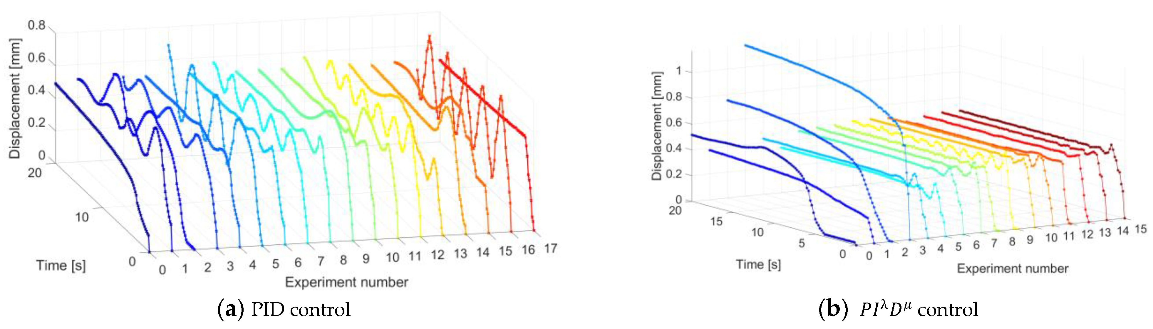
3.1. Step Responses of the Real DEA with PID and P I λ D μ Control

The step responses of the DEA were separated into step responses with PID control and step responses with P I λ D μ control. Figure 11 shows the step responses of individual sets of PID parameters. Eighteen experiments were performed, where different parameters were used. Promising parameters were experimented multiple times. Response time and settling time were measured as well as overshoot (P[%]) and steady-state error. Table 3 shows the results of the step responses of the DEA with PID control. It can be seen from Figure 11 that not all successful step responses performed in the Laplace domain and in the Simulink model gave good results with the real DEA. The best results were obtained with the experiments of numbers 4, 6, 8, 10, and 17. The average rise time was 1.9 s. The average settling time was 10.4 s. The average overshoot was 8.1% of the desired value. Some experiments also produced a steady-state error. The best performers in Table 3 are marked with the same color as in Figure 11a.
Figure 11b shows the step responses of the P I λ D μ control of the real DEA. An integral windup problem can be seen at the first four experiment numbers. In some experiments (4 to 9) the integral windup problem did not occur, but this did not guarantee the stability of the controller. Experiments with numbers 10 to 15 show step responses with the quasi-anti-windup method applied. The results were greatly improved, as rise times and settling times were reduced, and overshoots were reduced to an average 2.6% of the desired value. Table 4 shows the parameters used for individual experiments, as well as the results. The best results are highlighted with the same color as in Figure 11b.

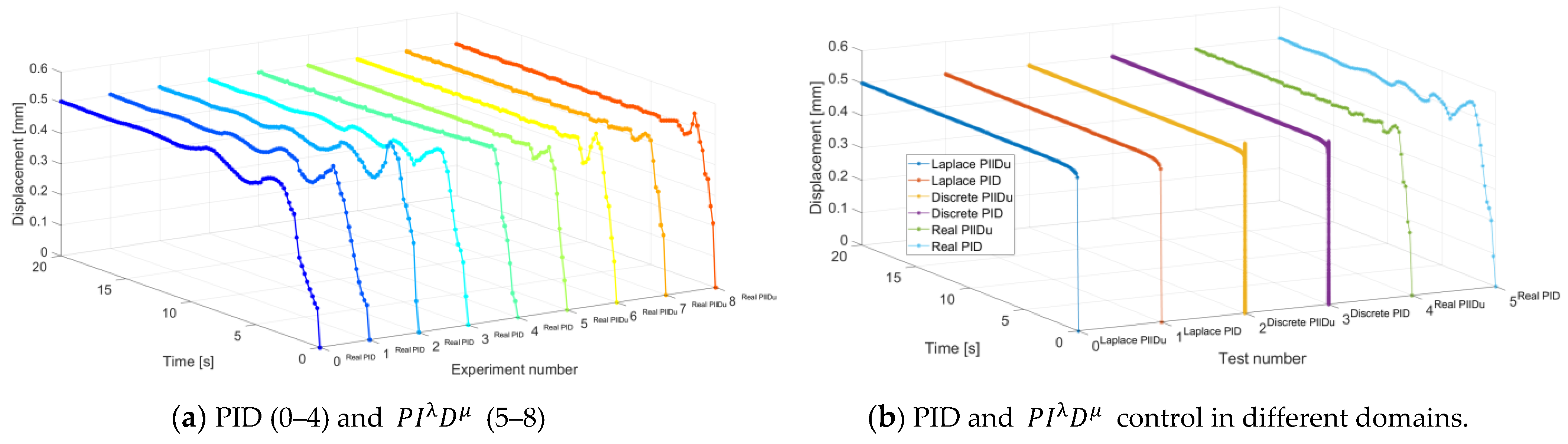
3.2. Comparing Results of Step Responses for Both Controllers and the Best Parameters in All Domains

Figure 12 shows the comparison of the step responses of both controllers for a real DEA. PID controller results are marked with experiment numbers 0 to 4, and P I λ D μ controller results are marked with experiment numbers 5 to 9. The best parameters for PID control were obtained by the Wuan–Juang–Chan algorithm. Average rise time among step responses with the PID controller was 1.7 s, the average settling time was 10.4 s, and the average overshoot was 8% of the desired value. On the other hand, these gain parameters were also the best for the P I λ D μ control where integration and derivation orders were optimized with help of the FOMCON toolbox. Table 5 shows the comparison of the results of the step responses obtained with both controllers. It can be seen that the P I λ D μ control improved step responses compared to the PID. For the P I λ D μ control the average rise time was reduced to 1 s, settling time to 5.4 s, and overshoot to 4.3%. With the implementation of the P I λ D μ control a small steady-state error was introduced, which was not greater than 1% and did not affect the controller’s performance significantly. When the order of integration in the P I λ D μ controller was less than 1, steady-state error was introduced to the step response of the plant.
Figure 12b shows the comparison of step responses with the same parameters of PID and P I λ D μ control in different domains. These parameters were K p = 5.66 ,   K i = 7.17 , K d = 0.03, λ = 0.6 , and μ = 0.8 . The best results were obtained for experiments 0 and 1, representing the Laplace domain, where the rise and settling times were the smallest and there was no overshoot. The reason is that the output of the controller was not saturated between 0 and 1.5 as it was in the Simulink models. The discrete Simulink models had slightly greater response and settling time as well as overshoot, as seen for experiments 2 and 3. Experiments 4 and 5 show the experimental results of the P I λ D μ and the PID control on the real DEA, respectively. Table 6 shows the response time, settling time, overshoot, and steady-state error of the step responses of controllers in different domains.

4. Discussion

The employment of fractional calculus in control theory can improve the P I λ D μ control of the fractional plant. The main objective was to eliminate the overshoot and make the response as fast as possible for the DEA, which was modeled as fractional plant. The easiest way to test fractional plant is in the Laplace domain. With the help of the Laplace transform, fractional derivates are transformed to fractional multiplication and fractional integrals into fractional division. Step responses performed in the Laplace domain gave the best results. However, the output of the fractional controller in the Laplace domain represents the force acting on the DEA plant. If the output is not saturated, then this output can also be negative, which helps reduce the settling time and overshoot of the DEA plant. But this is not the case in real application. When performing the experiment, the only force acting on retracting the DEA to its initial displacement were its internal polymer chains. That is the reason why continuous and discrete models in Simulink must be saturated between 0 and 1.5, which represent the force in N. The introduction of the saturated output of the controller had some negative effects on the step response. It reduced the response time and the settling time and increased the overshoot in the Simulink simulations.
Approximation of the P I λ D μ controller with high order Oustaloup filter is needed to perform a Simulink simulation. Continuous simulation was performed with a variable step solver in Simulink. For discrete simulation, a fixed step was chosen, corresponding to the microprocessor step. The size of the fixed step for discrete Simulink simulation must be properly chosen. Greater step size caused larger response time, settling time, and overshoots in discrete Simulink simulation.
To implement the P I λ D μ to the microprocessor it must be approximated with an Oustaloup filter in transfer function form and transformed into the z-domain with the same step as defined in the microprocessor. The first position control experiments of the DEA actuator resulted in large overshoot with a large steady-state error. This implied an integral windup problem. A quasi-anti-windup method was introduced to reset the transfer function of the P I λ D μ when the output exceeded a threshold value. As shown by the results, successful implementation and realization of the P I λ D μ position control was achieved for the selected DEA. Rise time was reduced by nearly half to around 1 s, as was settling time, which was reduced to around 5 s. Overshoot was also much lower, averaging around 4% of the final value. The main disadvantage of the P I λ D μ controller was the appearance of a steady-state error, even though the error was smaller than 1% of the desired value and did not influence the performance of the controller.
Observing the transition from the Laplace to the discrete domain, one can conclude that overshoot in step response in the Laplace domain predicts even greater overshoot in step response in continuous and discrete domains for the DEA plant. Controller output in the Laplace domain is not limited as it is in continuous and discrete domains between 0 and 1.5 and can also have negative values, which reduces the overshoot. If overshoot cannot be eliminated with unlimited output of the controller in the Laplace domain, then one can expect overshoot in continuous and discrete domains.
In future work, an anti-windup method with a transfer function for P I λ D μ approximation is going to be realized, separated into individual blocks of the z-transform. Each block will be limited with the output. Hopefully this will bring in even better results for position control.

Supplementary Materials

The following are available online at https://www.mdpi.com/2076-0825/10/1/18/s1.

Author Contributions

Conceptualization, methodology, software, validation, visualization, writing—review and editing, T.K. and J.G. All authors have read and agreed to the published version of the manuscript.

Funding

Authors acknowledges the financial support from Ministry of Education, Science and Sport and European Regional Development Fund Investing in Your Future. Part of this research was done under ROBKONCEL OP20.03530 project.

Institutional Review Board Statement

Not applicable.

Informed Consent Statement

Not applicable.

Data Availability Statement

All the research data are shown in the supplementary materials. Or please contact with the corresponding author: [email protected].

Conflicts of Interest

The authors declare no conflict of interest.

References

  1. Biewener, A.; Patek, S. Animal Locomotion; OUP: Oxford, UK, 2018. [Google Scholar]
  2. Punning, A.; Kim, K.J.; Palmre, V.; Vidal, F.; Plesse, C.; Festin, N.; Maziz, A.; Asaka, K.; Sugino, T.; Alici, G.; et al. Ionic electroactive polymer artificial muscles in space applications. Sci. Rep. 2014, 4, 6913. [Google Scholar] [CrossRef] [PubMed] [Green Version]
  3. Bar-Cohen, Y. Electroactive Polymer (EAP) Actuators as Artificial Muscles: Reality, Potential, and Challenges; SPIE Press: Bellingham, DC, USA, 2001. [Google Scholar]
  4. Leibniz, G.W. Mathematische Schiften; Georg Olms Verlagsbuchhandlung: Hildesheim, Germany, 1962. [Google Scholar]
  5. Podlubny, I. Fractional Differential Equations; Academic Press: San Diego, CA, USA, 1999; Volume 198, p. 311. [Google Scholar]
  6. Zambrano-Serrano, E.; Muñoz-Pacheco, J.M.; Gómez-Pavón, L.C.; Luis-Ramos, A.; Chen, G. Synchronization in a fractional-order model of pancreatic β-cells. Eur. Phys. J. Spec. Top. 2018, 227, 907–919. [Google Scholar] [CrossRef]
  7. Jesus, M.M.-P.; Cornelio, P.-C.; Ernesto, Z.-S. The Effect of a Non-Local Fractional Operator in an Asymmetrical Glucose-Insulin Regulatory System: Analysis, Synchronization and Electronic Implementation. Symmetry 2020, 12, 1395. [Google Scholar]
  8. Sun, H.; Zhang, Y.; Baleanu, D.; Chen, W.; Chen, Y. A new collection of real world applications of fractional calculus in science and engineering. Commun. Nonlinear Sci. Numer. Simul. 2018, 64, 213–231. [Google Scholar] [CrossRef]
  9. Tavazoei, M.S. Fractional order chaotic systems: History, achievements, applications, and future challenges. Eur. Phys. J. Spec. Top. 2020, 229, 887–904. [Google Scholar] [CrossRef]
  10. Mainardi, F.; Spada, G. Creep, relaxation and viscosity properties for basic fractional models in rheology. Eur. Phys. J. Spec. Top. 2011, 193, 133–160. [Google Scholar] [CrossRef] [Green Version]
  11. Caponetto, R.; Dongola, G.; Fortuna, L.; Petrá, I. Fractional Order Systems; World Scientific: Singapore, 2010; Volume 72. [Google Scholar]
  12. Petráš, I. Fractional-Order Nonlinear Systems: Modeling, Analysis and Simulation; Springer: New York, NY, USA, 2011. [Google Scholar]
  13. Babič, M.; Vertechy, R.; Berselli, G.; Lenarčič, J.; Parenti Castelli, V.; Vassura, G. An electronic driver for improving the open and closed loop electro-mechanical response of Dielectric Elastomer actuators. Mechatronics 2010, 20, 201–212. [Google Scholar] [CrossRef]
  14. Sarban, R.; Jones, R. Physical Model-Based Active Vibration Control using a Dielectric Elastomer Actuator. J. Intell. Mater. Syst. Struct. 2012, 23, 473–483. [Google Scholar] [CrossRef]
  15. Li, Y.; Oh, I.; Chen, J.; Zhang, H.; Hu, Y. Nonlinear dynamic analysis and active control of visco-hyperelastic dielectric elastomer membrane. Int. J. Solids Struct. 2018, 152, 28–38. [Google Scholar] [CrossRef]
  16. Nguyen, C.; Vuong, N.; Kim, D.; Moon, H.; Koo, J.; Lee, Y.; Nam, J.-D.; Choi, H.R. Fabrication and Control of Rectilinear Artificial Muscle Actuator. Mechatron. IEEE/ASME Trans. 2011, 16, 167–176. [Google Scholar]
  17. Mustaza, S.M.; Lekakou, C.; Saaj, C.; Fras, J. Dynamic Modeling of Fiber-Reinforced Soft Manipulator: A Visco-Hyperelastic Material-Based Continuum Mechanics Approach. Soft Robot. 2019, 6, 305–317. [Google Scholar] [CrossRef] [PubMed] [Green Version]
  18. Yeoh, O.H. Characterization of Elastic Properties of Carbon-Black-Filled Rubber Vulcanizates. Rubber Chem. Technol. 1990, 63, 792–805. [Google Scholar] [CrossRef]
  19. Cao, J.; Liang, W.; Ren, Q.; Gupta, U.; Chen, F.; Zhu, J. Modelling and Control of a Novel Soft Crawling Robot Based on a Dielectric Elastomer Actuator. In Proceedings of the 2018 IEEE International Conference on Robotics and Automation (ICRA), Brisbane, Australia, 21–25 May 2018; pp. 1–9. [Google Scholar]
  20. Rizzello, G.; Naso, D.; York, A.; Seelecke, S. Modeling, Identification, and Control of a Dielectric Electro-Active Polymer Positioning System. IEEE Trans. Control Syst. Technol. 2015, 23, 632–643. [Google Scholar] [CrossRef]
  21. Rizzello, G.; Naso, D.; York, A.; Seelecke, S. Closed loop control of dielectric elastomer actuators based on self-sensing displacement feedback. Smart Mater. Struct. 2016, 25, 035034. [Google Scholar] [CrossRef]
  22. FOMCON. FOMCON Toolbox for Matlab. Available online: http://fomcon.net/ (accessed on 10 December 2020).
  23. Xue, D.; Chen, Y.; Atherton, D. Linear Feedback Control: Analysis and Design with MATLAB (Advances in Design and Control); Society for Industrial and Applied Mathematics: Philadelphia, PA, USA, 2008. [Google Scholar]
  24. 3M™. 3M™ VHB™ Tape 4910. Available online: http://www.3m.com/3M/en_US/company-us/all-3m-products/~/3M-VHB-Tape-4910?N=5002385+3293242444&rt=rud (accessed on 24 July 2020).
  25. Conductive, B. Electric Paint. Available online: https://www.bareconductive.com/shop/electric-paint-50ml/ (accessed on 11 July 2020).
  26. Mainardi, F. Fractional Calculus and Waves in Linear Viscoelasticity: An Introduction to Mathematical Models; Imperial College Press: London, UK, 2010; pp. 51–63. [Google Scholar]
  27. Lewandowski, R.; Chorążyczewski, B. Identification of the parameters of the Kelvin-Voigt and the Maxwell fractional models, used to modeling of viscoelastic dampers. Comput. Struct. 2010, 88, 1–17. [Google Scholar] [CrossRef]
  28. Diethelm, K. The Analysis of Fractional Differential Equations: An Application-Oriented Exposition Using Differential Operators of Caputo Type; Springer: Berlin/Heidelberg, Germany, 2010. [Google Scholar]
  29. Timi, K.; Tomaž, V.; Janez, G.; Boštjan, R.; Karl, G. Parameters identification method for viscoelastic dielectric elastomer actuator materials using fractional derivatives. Mater. Res. Express 2018, 5, 075702. [Google Scholar]
  30. Karner, T.; Gotlih, J.; Razboršek, B.; Vuherer, T.; Berus, L.; Gotlih, K. Use of single and double fractional Kelvin-Voigt model on viscoelastic elastomer. Smart Mater. Struct. 2019, 29, 015006. [Google Scholar] [CrossRef]
  31. Monje, C.; Chen, Y.; Vinagre, B.; Xue, D.; Feliu, V. Fractional Order Systems and Control—Fundamentals and Applications; Springer Science & Business Media: Berlin/Heidelberg, Germany, 2010. [Google Scholar]
  32. Xue, D. FOFT Toolbox. Available online: https://www.mathworks.com/matlabcentral/fileexchange/60874-fotf-toolbox (accessed on 7 August 2020).
  33. Tepljakov, A. Fractional-Order Modeling and Control of Dynamic Systems; Springer International Publishing: Berlin/Heidelberg, Germany, 2017. [Google Scholar]
  34. Karner, T.; Žefran, M.; Gotlih, K. Using Fractional Derivatives for Parameter Identification and Control of Dielectric Elastomer Actuators; Springer: Cham, Switzerland, 2019; pp. 2469–2479. [Google Scholar]
  35. Lewis, R.M.; Torczon, V.; Trosset, M.W. Direct search methods: Then and now. J. Comput. Appl. Math. 2000, 124, 191–207. [Google Scholar] [CrossRef] [Green Version]
  36. Sabatier, J.L.; Melchior, P.; Oustaloup, A. Fractional Order Differentiation and Robust Control Design: CRONE, H-infinity and Motion Control; Springer: Dordrecht, The Netherlands, 2015. [Google Scholar]
  37. Hackl, C.M.; Tang, H.-Y.; Lorenz, R.D.; Turng, L.-S.; Schroder, D. A Multidomain Model of Planar Electro-Active Polymer Actuators. IEEE Trans. Ind. Appl. 2005, 41, 1142–1148. [Google Scholar] [CrossRef]
  38. TMS320F28069M. Texas Instruments. Available online: http://www.ti.com/product/TMS320F28069M (accessed on 23 October 2020).
  39. Wenglor. YP05MGV80. Available online: https://www.google.com/url?sa=t&rct=j&q=&esrc=s&source=web&cd=1&ved=2ahUKEwihnaWa0bbjAhXiB50JHWepBx0QFjAAegQIBhAC&url=http%3A%2F%2Fwww.shintron.com.tw%2Fproimages%2Ftakex%2Fwenglor%2FYP05MGV80.pdf&usg=AOvVaw0hZdH3GNiqDLpm9BclkSVw (accessed on 15 July 2020).
  40. Design, A. E1 Series 1 Watt. Available online: http://apowerdesign.com/products/E/E1/ (accessed on 23 October 2020).
Figure 1. Basic structure of a planar DEA: (a) deactivated state and (b) activated state.
Actuators 10 00018 g001
Figure 2. Stretched elastomer on the left and active surface of the DEA on the right.
Actuators 10 00018 g002
Figure 3. Poles of the commensurate order transfer function of fractional Kelvin-Voigt model.
Actuators 10 00018 g003
Figure 4. Difference in Bode diagrams of the fractional and the basic Kelvin-Voigt model.
Actuators 10 00018 g004
Figure 5. Step response of plant model with the PID and P I λ D μ controller.
Actuators 10 00018 g005
Figure 6. Simulink model for DSP implementation with serial communication.
Actuators 10 00018 g006
Figure 7. Reading real time measurements from DSP in Matlab/Simulink.
Actuators 10 00018 g007
Figure 8. Simulink block inside the ADC_ISR block.
Actuators 10 00018 g008
Figure 9. Simulink model of the fractional control algorithm with the quasi-anti-windup method.
Actuators 10 00018 g009
Figure 10. Experimental setup of the real DEA or the plant model for simulations.
Actuators 10 00018 g010
Figure 11. Step responses of a real DEA using (a) a PID control and (b) a P I λ D μ control.
Actuators 10 00018 g011
Figure 12. Comparison of the step responses of (a) the PID (0–4) and P I λ D μ (5–8) control of a real DEA and comparison of step responses of (b) the PID and P I λ D μ control in different domains.
Actuators 10 00018 g012
Table 1. Initial, optimal, and comparing parameters of the P I λ D μ and PID and their step responses in the Laplace domain.
K p K i K d λμ T r [ s ] T s [ s ] P [ % ]
P I λ D μ Initial param.1110.50.5
Optimal param.06.580.530.50.50.0140.920
PIDComp. parameters06.580.53110.0048.9810.8
P I λ D μ Initial param.1110.50.5
Optimal param.3.461000.160.470.810.0070.043
PIDComp. parameters3.461000.16110.0090.221.6
P I λ D μ Initial param.1110.50.5
Optimal param.1110.090.70.0041.935
PIDComp. parameters111110.0045.91.62
P I λ D μ Initial param.5.667.170.030.50.5
Optimal param.023.181.250.50.50.0140.920
PIDComp. parameters023.181.25110.0049.493.6
P I λ D μ Initial param.5.667.170.030.50.5
Optimal param.1.911000.180.460.790.0110.042.8
PIDComp. parameters1.911000.18110.0120.243
P I λ D μ Initial param.5.667.170.030.50.5
Optimal param.5.667.170.030.860.90.010.750
PIDComp. parameters5.667.170.03110.0150.750
P I λ D μ averages0.0100.771.16
PID averages0.0084.263.44
Table 2. Comparison of the step response of the DEA in the different domains of controller models.
Laplace TFSimulink Contin.Simulink Discrete
K p K i K d λμ T r [ s ] T s [ s ] P [ % ] T r [ s ] T s [ s ] P [ % ] T r [ s ] T s [ s ] P [ % ]
PID06.580.53110.0048.9810.80.389.9470.389.668
P I λ D μ 06.580.530.50.50.0140.9200.0141280.0140.8515
PID3.461000.16110.0090.221.60.040.42300.040.4230
P I λ D μ 3.461000.160.470.810.0070.0430.010.12460.010.1243
PID1.911000.18110.0920.243.100.050.75480.0500.7548
P I λ D μ 1.911000.180.460.790.0080.042.800.0100.11450.0100.1142
PID5.667.170.03110.0110.750.000.050.3610.050.351
P I λ D μ 5.667.170.030.860.90.010.750.500.020.3000.020.311
PID111110.0045.91.621.248.20201.248.2020
P I λ D μ 1110.090.70.0041.9350.358.4210.482.56No.
PID023.11.25110.0049.493.60.289.90960.2209.9090
P I λ D μ 023.11.250.50.50.0090.2200.0150.2340.0400.222
Table 3. Step responses of a real DEA using a PID control with different parameters.
Exp. Number K p K i K d T r [ s ] T s [ s ] R [%]Steady-State Error
05.60.037.115.831.72.8No
15.67.10.03224.833.1No
2023.11.23.2No32.9Yes
33.41000.12.5No19.4Yes
45.67.10.032.79.44.3No
5023.11.21.8No51.18Yes
65.67.11002.3115No
70.17.11002.3No19.7Yes
85.67.11001.310.717.4No
96363611.214.433.6No
105.67.10.031.59.17.9No
115.57.10.031.7No30.6Yes
123.41000.11.4No25.2Yes
13023.11.26.123.618No
14023.11.22.225.234.2Yes
15023.11.24.824.124.2No
16023.11.21.2No54.8Yes
175.67.10.031.511.86No
Table 4. Step responses of a real DEA using P I λ D μ with different parameters, part 1.
Exp. K p K i K d λμ T r [ s ] T s [ s ] R [%]Steady-State Error
03.41000.160.470.812.733.613.4Yes
11.91000.180.460.79No400Yes
25.67.10.030.860.92.74054.7Yes
35.67.10.030.860.9140146Yes
45.67.10.030.860.91.2400Yes
51.911000.180.470.81No100Yes
65.67.10.030.980.91.4250Yes
75.623.10.030.860.91300Yes
8023.10.030.50.51.1100Yes
9023.11.20.50.512514.2Yes
10023.11.20.50.514.22.2Yes
115.67.10.030.860.917.45.41%
125.67.10.030.90.91150Yes
135.67.10.030.60.91150Yes
145.67.10.030.60.815.80<1%
155.67.10.030.50.914.391%
Table 5. Comparison of the step responses of the PID (0–4) and P I λ D μ (5–8) control of a real DEA.
Exp. K p K i K d λμ T r [ s ] T s [ s ] Overshoot [%]Steady-State Error
05.67.10.03112.49.44.3No
15.67.10.03112.1115No
25.67.10.03111.310.717.4No
35.67.10.03111.49.17.8No
45.67.10.03111.311.86No
55.623.11.20.50.514.22.2No
65.67.10.030.860.917.45.41%
75.67.10.030.60.815.80.6<1%
85.67.10.030.50.91.14.391%
Table 6. Comparison of step responses with PID and P I λ D μ control in different domains.
Exp. K p K i K d λμ T r [ s ] T s [ s ] Overshoot [%]Steady-State Error
05.67.10.030.80.90.120.410No
15.67.10.03110.130.440No
25.67.10.030.8680.90.090.445No
35.67.10.03110.090.683No
45.67.10.030.60.81.135.840.6<1%
55.67.10.03111.549.147.8No
Publisher’s Note: MDPI stays neutral with regard to jurisdictional claims in published maps and institutional affiliations.

