Improved Method for Distributed Parameter Model of Solenoid Valve Based on Kriging Basis Function Predictive Identification Program

Abstract

In this paper, a method for the improvement of the calculation accuracy of the distributed parameter model (DPM) of electromagnetic devices is proposed based on the kriging basis function predictive identification program (PIP). Kriging is mainly an optimal interpolation method which uses spatial self-covariance, and takes a polynomial as the basis function. The accuracy of the kriging-based surrogate model can be improved by adjusting the related functions and hyperparameters. Based on the DPM of a solenoid valve, there exist certain errors in the estimation. They can be summarized as follows: Firstly, the estimation error of magnetic flux leakage (MFL) permeance is caused directly by the deviation of the magnetic flux tube due to the segmented magnetic field line. Secondly, the estimation error of soft magnetic resistance because of the nonlinearity of the permeability of soft magnetic material leads to the change of soft magnetic resistance alongside the magnetic flux. In this paper, an improved kriging error correction method is applied to modify the leak permeance and soft magnetic resistance calculation. The kriging basis function is adjusted to adapt to the data curve of the MFL permeance error data. The calculated MFL permeance data are compared with the error variation data to select the appropriate basis function. To improve the computational efficiency, the PIP is proposed to select the appropriate basis function. The modified MFL permeance data and soft magnetic resistance are substituted into the DPM for improving the computational accuracy and efficiency of the solenoid valve.

1. Introduction

The optimization design of modern solenoid valves faces more and more challenges with increasing performance requirements to realize higher latching force, higher output force, and more extensive robustness [1,2,3,4,5,6,7,8,9]. As a means of simulation, the FEM method has the absolute advantage of accuracy, and the disadvantage of efficiency. The distributed parameter model (DPM) method can effectively speed up the calculation, and kriging models can decrease error. The DPM and kriging models have become important factors affecting the design efficiency and accuracy of solenoid valves. Therefore, evaluating the applicability of the kriging model has an important theoretical significance and a practical engineering value for product design optimization [10,11,12,13,14,15].

With the increasing levels of computational technology and theoretical analysis for the DPM, the kriging model, whose inputs affect its outputs, plays an important role in engineering design and error correction [16,17,18,19,20,21]. The calculation accuracy of air leakage permeance and the soft magnetic resistance has an effect on the electromagnetic force calculation accuracy of solenoid valves. To reduce the relative error and improve the accuracy of target prediction based on sample data, various data fitting methods based on the kriging model have been proposed. In the design and optimization of products, kriging has a good performance in error correction [22,23,24,25,26,27,28]. An adaptive finite difference weighted essentially non-oscillatory (WENO) method with Gauss-kriging reconstruction is proposed to reduce dissipation in smooth regions of flow, while preserving high resolution around discontinuities for hyperbolic systems of conservation laws [29]. The work in [30] proposed a kriging model-based method for the reliability design and optimization of planetary gear, using a genetic algorithm. The kriging model was used to establish the gear reliability model to simplify the reliability calculation in this method [30]. Shin et al. performed an optimization study of response time to improve the dynamic performance of a direct-acting solenoid valve based on a kriging model [31]. A kriging metamodel-based multi-objective optimization strategy has been employed to optimize the valve-plate shape of the axial piston pump [32]. The kriging method was also used to build a surrogate model, which presents the relationship between dynamic responses and dynamic simulation of the valve train [33]. Many of the works where the kriging model has been adopted for error calculation mainly focus on the calculation errors associated with replacing the original analytical model with the kriging-based surrogate model.

In this paper, a method for the improvement of the calculation efficiency and accuracy of the DPM of electromagnetic devices is proposed based on the kriging basis function predictive identification program (PIP). To obtain an improved DPM performance, an appropriate basis function is selected by contrasting various basis functions with error item curves of air leakage permeance. To further improve the calculation efficiency, the PIP is introduced to prejudge the error item curves against standard functions. The modified leakage permeance and the soft magnetic resistance data are considered in the DPM of the electromagnetic device to calculate the electromagnetic force, thereby verifying the method proposed in this paper.

2. The Error Correction Method of DPM Based on Kriging Model

The kriging model is a global surrogate model derived from geostatistics, and it can mathematically provide an optimal linear unbiased estimation. This makes it an appropriate method to achieve the primary goal of this paper. To estimate the linear, unbiased and minimum estimated variance using kriging, the geometric features of information sample shape, size and space on samples are taken into account. Nonetheless, kriging is still a smooth interpolation method [34,35]. The electromagnetic calculation software is Matlab in this paper.

The kriging model can be summarized in two parts, which are represented by

$$y(x)={\displaystyle \sum _{j=1}^p{\beta }_j{f}_j(x)+Z(x)}$$

(1)

where f_j(x) is the basis, β_j is the regression coefficient, Z(x) is the stochastic distribution function.

A solenoid valve with a fan-shaped permanent magnet (PM) is selected as the example in this study, and its electromagnetic system is shown in Figure 1. The armature is a moving part, the angle of the fan-shaped PM is 20°, its inner radius is 8.5 mm, its outer radius is 17.5 mm and its height is 8 mm. The solenoid valve rated coil ampere-turns equal 1800 AT. The PM is divided into seven segments. The magnetic flux leakage (MFL) permeances of the flux tube from the outer radius side to the inner radius side are G₁, G₂, G₃, G₄, G₅, G₆ and G₇ [36,37,38,39,40].

The solenoid valve is excited in 0 AT, and its finite element method (FEM) responses are compared with the unmodified DPM, as shown in Figure 2. There are 20 sample points for every curve.

The FEM and DPM data are subtracted to obtain the MFL permeance error terms (i.e., ΔG₁, ΔG₂, ΔG₃, ΔG₄, ΔG₅, ΔG₆ and ΔG₇), which are then stored in the error matrix Er. The MFL permeance data are shown in Figure 3 which reveal a non-monotonic variation.

To further improve the error correction efficiency, multi-basis functions are applied to the adaptive error curve. The kriging basis functions are represented as follows:

Fourier Function

$$f(x)={\displaystyle \sum _i^n[a_i\sin (d_{i}wi)+b_i\sin (d_{i}wi)]}.$$

(2)

Polynomial Function

$$f(x)=1+{\displaystyle \sum _{i=1}^n{d}_i}+{\displaystyle \sum _{i=1}^n{d}_i^2}+{\displaystyle \sum {\displaystyle \sum _{i<j}{d}_i{d}_j}}.$$

(3)

Exponential Function

$$f(x)=e^{{\displaystyle \sum _{i=1}^n(-{\theta }_i,\left|d_j\right|)}}.$$

(4)

Gaussian Function

$$f(x)=e^{{\displaystyle \sum _{i=1}^n(-{\theta }_i,{\left|d_j\right|}^2)}},$$

(5)

where |d_i| is the distance between the known and predicted quantities.

The basis function output characteristics can be determined using the key nodes and the output of the model. Given a function k(x₁, x₂… x_n) and an input parameter x₁, x₂… x_n, the domain of the function can be expressed as follows:

$$\{\begin{array}{c}{X}_1\in [x_1^0-\Delta x_1,x_1^0+\Delta x_1]\\ X_2\in [x_2^0-\Delta x_2,x_2^0+\Delta x_2]\\ ⋮\\ X_n\in [x_n^0-\Delta x_n,x_n^0+\Delta x_n]\end{array},$$

(6)

where x₁, x₂… x_n are the coordinate positions of magnetic lines of flux with armature displacement, x₁₀, x₂₀… x_n0 are the center of fluctuations, Δx₁, Δx₂… Δx_n are the ranges of fluctuations. The basis function can be simplified to:

$$\Delta F\approx {\displaystyle \sum _{i=1}^n\Delta F_i}+{\Delta }^2(\Delta x),$$

(7)

where ΔF is the function output, Δ²(Δx) is the higher derivative of the input parameter fluctuations. Given that a function relation exists between k(x₁, x₂… x_n) and Δx₁, Δx₂… Δx_n, k(x₁, x₂… x_n), this function relation can be described as follows:

$$k\left(x_1^0,x_2^0\dots x_n^0\right)={\displaystyle \sum _{x_1^0-\Delta x_1,x_2^0-\Delta x_2\dots x_n^0-\Delta x_n}^{x_1^0+\Delta x_1,x_2^0+\Delta x_2\dots x_n^0+\Delta x_n}k\left(x_1,x_2\dots x_n\right)w|{}_{x_1,x_2\dots x_n}},$$

(8)

where w is the weight coefficient. For every node in the count, w = 1. However, if the sample points are not key nodes, then 0 < w < 1. Given that, the boundary condition of the input parameter is as follows:

$$\{\begin{array}{c}{x}_{1l}\le x_1\le x_{1h}\\ x_{2l}\le x_2\le x_{2h}\\ ⋮\\ x_{nl}\le x_n\le x_{nh}\end{array},$$

(9)

where x_il, x_ih are the top and bottom limitations of the ith input value. Combining Equations (7)–(9), ΔF_i can be defined as:

$$\Delta F_i={\displaystyle \sum _{(x_{lh},x_{lh}\dots x_{lh})}^{(x_{1h},x_{2h}\dots x_{nh})}w\Delta F(\Delta x_i)}|{}_{x_1,x_2\dots x_n}G(x_1,x_2\dots x_n)|{}_{x_1^0,x_2^0\dots x_n^0},$$

(10)

where G(x₁, x₂… x_n) is the interpolating function of x₁, x₂… x_n. Substituting G(x₁, x₂… x_n) into Equations (7) and (8), the following equations are obtained:

$${G(x_1,x_2\dots x_n)|}_{\left(x_1^0,x_2^0\dots x_n^0\right)}=e^{{\displaystyle \sum _{i=1}^n(-{\theta }_i,\left|d_i\right|)}},$$

(11)

$${G(x_1,x_2\dots x_n)|}_{\left(x_1^0,x_2^0\dots x_n^0\right)}=e^{{\displaystyle \sum _{i=1}^n(-{\theta }_i,{\left|d_i\right|}^2)}},$$

(12)

where $d_i=\left|x-x_i\right|$, x is the dependent variable, θ_i is the PM segment positions with respect to the armature displacement. The armature stroke is 2 mm, and θ_i can be obtained by particle swarm optimization (PSO) based on 20 nodes.

Based on the MFL permeance error data, and adopting a periodic function (i.e., Fourier series) for ΔG₃ fitting, it can be written as follows:

$$f(x)=a_0+{\displaystyle \sum _{i=1}^4[a_i\cos (ixw)+b_i\sin (ixw)]},$$

(13)

where x is the armature stroke, f(x) is the dependent variable of the MFL permeance. a₀ = −857, a₁ = 1384, b₁ = −45.96, a₂ = −71.14, b₂ = 43.84, a₃ = 212.3, b₃ = −17.28, a₄ = −28.1, b₄ = 2.529, w = 0.1202. Taking the derivative of Equation (13), df(x)/dx has four solutions defined in the range 0 to 2.

By adopting a polynomial function for ΔG₃ fitting, it can be written as follows:

$$f(x)=p_1{x}^7+p_2{x}^6+p_3{x}^5+p_4{x}^4+p_5{x}^3+p_6{x}^2+p_{7}x+p_8,$$

(14)

where p₁ = −5.34 × 10⁻⁶, p₂ = 3.26 × 10⁻⁵, p₃ = −7.49 × 10⁻⁵, p₄ = 8.1 × 10⁻⁵, p₅ = −4.26 × 10⁻⁵, p₆ = 1.08 × 10⁻⁶, p₇ = −1.33 × 10⁻⁶, p₈ = −3.92 × 10⁻⁸. Taking the derivative of Equation (14), i.e., df(x)/dx, yields four solutions.

By adopting an exponential function for ΔG₃ fitting, it can be written as follows:

$$f(x)=a{e}^{bx}+c{e}^{dx},$$

(15)

where a = −7.591 × 10⁻⁷, b = 4.862, c = 7.583 × 10⁻⁷, d = 4.863. Taking the derivative of Equation (15), i.e., df(x)/dx, has only one solution. It is obvious that the exponent is unfit for ΔG₃ fitting.

By adopting a Gaussian function for ΔG₃ fitting, it can be written as follows:

$$f(x)=a_1{e}^{-\frac{{(x-b_1)}^2}{2c_1^2}}+a_2{e}^{-\frac{{(x-b_2)}^2}{2c_2^2}}+a_3{e}^{-\frac{{(x-b_3)}^2}{2c_3^2}}+a_4{e}^{-\frac{{(x-b_4)}^2}{2c_4^2}}+a_5{e}^{-\frac{{(x-b_5)}^2}{2c_5^2}},$$

(16)

where a₁ = 1.28 × 10⁻⁶, b₁ = 1.906, c₁ = 0.2655, a₂ = 0, b₂ = 10.97, c₂ = 0.03011, a₃ = 2.89 × 10⁻⁵, b₃ = 1.29, c₃ = 0.6738, a₄ = −2.87 × 10⁻⁵, b₄ = 1.302, c₄ = 0.6887, a₅ = −0.6322 × 10⁻⁷, b₅ = 0.5452, c₅ = 0.1176. Taking the derivative of Equation (16), i.e., df(x)/dx, yields four solutions.

Figure 4 shows the contrasting condition between basis functions and MFL permeance error ΔG₃. It is obvious that there is a large error between the exponential function-based fitted curve and ΔG₃. The mean error for this particular case is over 100%. The polynomial function-based fitted curve, Fourier function-based fitted curve and Gaussian function-based fitted curve have mean errors reaching 38.4%, 30.1% and 14.2%, respectively.

To further improve computational efficiency, the reliability index of samples is calculated by four algorithms to achieve optimal basis function. The algorithms are:

• Particle Swarm Optimization(PSO)
• Response Surface (RS)
• Linear Second order moment (LS)
• Monte Carlo (MC)

The relative error of the basis functions can be obtained by taking MC as the base. Firstly, the failure probability of the samples is calculated, then the reliability index can be obtained using the calculation results. The reliability index is calculated by the MC method and it is used as the standard with a termination condition of 10⁻⁷.

Table 1. The basis function model reliability index of ΔG3.

Function	Algorithm	Iteration	Count	Time (s)
Gaussian	PSO	132	660	987
	RS	189	945	1229
	LS	147	588	1143
	MC	-	105	2961
Fourier	PSO	162	810	1328
	RS	198	990	1843
	LS	204	816	1687
	MC	-	105	3063
Polynomial	PSO	153	765	1125
	RS	207	1035	2063
	LS	192	768	1763
	MC	-	105	3012

shows the reliability index of ΔG₃.

Table 1 shows that Gaussian function with PSO has the smallest count for ΔG₃, while the Fourier function with PSO has the smallest count for ΔG₁.

ΔG₃ is presented as an example. The polynomial function is adopted for the armature stroke, Gaussian error data and ΔG₃. This function can be written as follows:

$$\Delta G_3=p_{00}+p_{10}x+p_{01}{y}^3+p_{20}x+p_{11}xy,$$

(17)

where p₀₀ = −2.057 × 10⁻⁷, p₁₀ = 7.069 × 10⁻⁷, p₀₁ = −0.02261, p₂₀ = −4.141 × 10⁻⁷, p₁₁ = 0.3128. x is the armature stroke, y is the Gaussian error data. Figure 5 shows Gaussian error data fitting.

The MFL permeance of the solenoid valve G₃ can be improved. Now, assuming that P is the FEM data matrix and Q is the DPM data matrix, Er can be written as follows:

Er = P − Q

(18)

If ΔG depicts the permeance error of the sampling point, Er can be derived as follows:

$$Er=\left[\begin{array}{llll}\Delta G_{11}& \Delta G_{12}& \cdots & \Delta G_{1m}\\ \Delta G_{21}& \ddots & & \Delta G_{2m}\\ ⋮& & \ddots & ⋮\\ \Delta G_{n1}& \Delta G_{n2}& \cdots & \Delta G_{nm}\end{array}\right],$$

(19)

where n is the PM segment number, m is the sampling point position. i = 1, 2, …n. j = 1, 2, …m.

The basis function can be defined as f_k(x₁, x₂…x_q), k = 1, 2, 3, …n, where q is the dimension. f_k(x₁, x₂…x_q). The function can be written as:

$$f\left(x_1,x_2,\dots ,x_q\right)=\min \left\{f_k\left(x_1,x_2,\dots ,x_q\right)-Er\left[k;\right]\right\}.$$

(20)

Based on Equation (20), the polynomial function is adopted for the armature stroke, l, ΔG and f(x₁, x₂…x_q). This function is written as follows:

$$\Delta G=p_{00}+p_{10}l+p_{01}{f}^3(x_1,x_2\dots x_q)+p_{20}l+p_{11}lf(x_1,x_2\dots x_q).$$

(21)

Equation (21) can also be written as follows:

$$f_{er}\left(l,x_1,x_2,\dots ,x_q\right)=X\left[\Delta G,l,f\left(x_1,x_2,\dots ,x_q\right)\right]$$

(22)

where f_er(l, x₁, x₂…x_q) is the penalty function for the error data of the sampling point with armature displacement. The ith MFL permeance or soft magnetic resistance can be defined as q_i(x), where x is the unknown quantity. Therefore, w_i(x) can be obtained as follows:

$$w_i(x)=f_{eri}(x)+q_i(x)$$

(23)

where w_i(x) is the improved DPM data, and it is very close to the FEM data.

3. MFL Permeance Prejudge the Error Data Based on Kriging PIP

To improve the overall calculation efficiency of the program, the predictive identification program is applied to prejudge the scatter data before employing the kriging base function.

The basis function can be defined as f(x), $a=(x_1,x_2,\dots x_n)\in R^n$, where f(x) is continuous and differentiable in the field of definition.

$$\nabla f(x)(x-a)<0,$$

(24)

where f(x) is the maximum with x = x_k.

Similarly,

$$\nabla f(x)(x-a)>0,$$

(25)

where f(x) is the minimum with x = x_k.

The extreme function can be analyzed according to Equations (24) and (25), and the gradient of f(x) can be written as follows:

$$\nabla f(x)={\left[\frac{\partial f(x)}{\partial x_1},\frac{\partial f(x)}{\partial x_2},\dots ,\frac{\partial f(x)}{\partial x_n}\right]}^T.$$

(26)

Based on the characteristic of the first derivative, the adjacent points x_i and x_i+1 are the local maxima or minima. Therefore, the adjacent points are used as the criteria to judge the curve of the function. If the adjacent points of the function data are monotonically increasing, and the second derivative product is positive, this shows that the function is unimodal and it has a maximum. Therefore, it can be obtained as follows:

$$\{\begin{array}{l}\frac{\partial f(x)}{\partial x_1}=0,\frac{\partial f(x)}{\partial x_2}=0,\dots ,\frac{\partial f(x)}{\partial x_n}=0\\ f(x_i)<f(x_{i+2})\\ f(x_{i+1})<f(x_{i+3})\\ \frac{{\partial }^2(x){\partial }^{2}f(x)}{{\partial }^2{x}_i{\partial }^2{x}_{i+2}}>0\end{array},$$

(27)

Similarly,

$$\{\begin{array}{l}\frac{\partial f(x)}{\partial x_1}=0,\frac{\partial f(x)}{\partial x_2}=0,\dots ,\frac{\partial f(x)}{\partial x_n}=0\\ f(x_i)>f(x_{i+2})\\ f(x_{i+1})>f(x_{i+3})\\ \frac{{\partial }^2(x){\partial }^{2}f(x)}{{\partial }^2{x}_i{\partial }^2{x}_{i+2}}>0\end{array}.$$

(28)

From Equation (28), the function is unimodal and has a minimum.

Similarly,

$$\{\begin{array}{l}f(x_i)<f(x_{i+2}),f(x_i)>f(x_{i+2})\\ \frac{\partial f(x)}{\partial x_1}=0,\frac{\partial f(x)}{\partial x_2}=0,\dots ,\frac{\partial f(x)}{\partial x_n}=0\\ f(x_{i+1})>f(x_{i+3}),f(x_{i+1})<f(x_{i+3})\end{array}.$$

(29)

If the adjacent points of the function data are monotonically increasing or decreasing, then the function has a multi-crest. As such, the derivative can identify the extremum of the scatter data, and the shape of the multi-crest based on the number of extremum points.

To identify the more complicated scatter data curve, the standard function for numerical matching of the scatter data is applied. When the trend of the curve for the standard function is the same as the trend of the distribution for the scatter data, it can be said that the corresponding kriging basis function is practical for this type of standard function.

Based on the trend of the ΔG_i curve, the Schwefel function has similar characteristics. Figure 6 shows the standard Schwefel function.

The Schwefel function can be written as follows:

$$f(x)=x\sin \left(\sqrt{\left|x\right|}\right)$$

(30)

From Equation (30), the parameters can be modified to have the following:

$$f(x)=-1-2.6x\sin \left(-3.8+15\sqrt{\left|x-0.02\right|}\right)$$

(31)

The Schwefel functions are compared with ΔG₃ and ΔG₄, as shown in Figure 7.

The similarity between the Schwefel function, ΔG₃ and ΔG₄ can be obtained using the Tanimoto method. This method is stated as follows:

$$T(x_1,x_2)=\frac{{\displaystyle \sum x_{1i}{x}_{2i}}}{{\displaystyle \sum x_{1i}^2+{\displaystyle \sum x_{2i}^2}-{\displaystyle \sum x_{1i}{x}_{2i}}}}$$

(32)

By calculation, the similarity of ΔG₃ with the Schwefel function is 0.7654, and the similarity of ΔG₄ with the Schwefel function is 0.7775. The similarities of ΔG with the Schwefel function are further detailed in

Table 2. Schwefel function and ΔG similarity.

Schwefel Similarity	ΔG1	ΔG2	ΔG3	ΔG4	ΔG5	ΔG6	ΔG7
	0.005	0.0662	0.7654	0.7775	0.1674	0.5698	0.0013

.

In Table 2, the similarities of ΔG₃ and ΔG₄ with the Schwefel function are over 0.7, while the similarities of other ΔG₁, ΔG₂, ΔG₅, ΔG₆ and ΔG₇ are the same as the trigonometric function. The similarities of ΔG are compared with the trigonometric function, as shown in

Table 3. Trigonometric function and ΔG similarity.

Trigonometric Similarity	ΔG1	ΔG2	ΔG3	ΔG4	ΔG5	ΔG6	ΔG7
	0.8625	0.921	0.231	0.1922	0.8124	0.7958	0.7642

.

It can be concluded that the similarities which are over 0.7 conform to the corresponding standard function. Hence, the kriging basis function can be selected. When the similarity of the ΔG curve and the Schwefel function is over 0.7, ΔG can be modified by the Gaussian function. When the similarity of the ΔG curve and the trigonometric function is over 0.7, ΔG can be modified by the Fourier function.

4. The Error Correction of MFL Permeance and Soft Magnetic Resistance of Solenoid Valves

To verify the practicality of the proposed method, the kriging model based on the basis function adjustment is used to modify the error of the MFL permeance and soft magnetic resistance data of the solenoid valve magnetic system. Substituting modified data into the DPM, the electromagnetic force can be obtained.

From Figure 8, it can be observed that the unmodified DPM permeance mean error reaches 13.1% (see Figure 2), and the modified DPM mean error reaches 4.7%.

The soft magnetic resistance in la₁ and la₂ segments is taken as an example, without the presence of an excitation current in the coil and at different armature positions. Figure 9 shows the soft magnetic resistance of FEM and the unmodified and modified DPM. The unmodified DPM permeance mean error reaches 9.94%, while the modified DPM permeance mean error reaches 3.7%.

The modified MFL permeance and soft magnetic resistance data are substituted into the DPM. The FEM results are compared with the modified and unmodified DPM results of the force on the armature for a coil excitation of 1800 AT and −1800 AT, as shown in Figure 10. The unmodified DPM mean error is 10.2%, and the modified DPM mean error is 3.8%. The FEM and measurement results mean error is 3%.

Figure 11 shows the flow chart of the improved method for the DPM of solenoid valves based on the kriging basis function PIP. An appropriate function is selected by the PIP for error correction, and by substituting modified data into the DPM, the electromagnetic force can be obtained. Under the same calculation conditions, the output force of one armature displacement point cost 420 s in the FEM, and 56 s in the DPM.

5. Conclusions

To improve the calculation accuracy and efficiency of the solenoid valve DPM, an improved method for the DPM based on the kriging basis function PIP is proposed in this paper. From the experiments and the results, the following conclusions are drawn:

• Based on the characteristics of the kriging basis function curve, the relationship between the kriging basis function and the MFL permeance error data can be obtained, and an appropriate function is selected by contrasting various basis functions with error data curves. Then it is applied to gain error compensation between the FEM and DMP data. The PIP is introduced to prejudge the error data by comparing the standard function to the selected basis function. The modified MFL permeance and the soft magnetic resistance data are then substituted into the DPM of the electromagnetic device to calculate the attraction force.
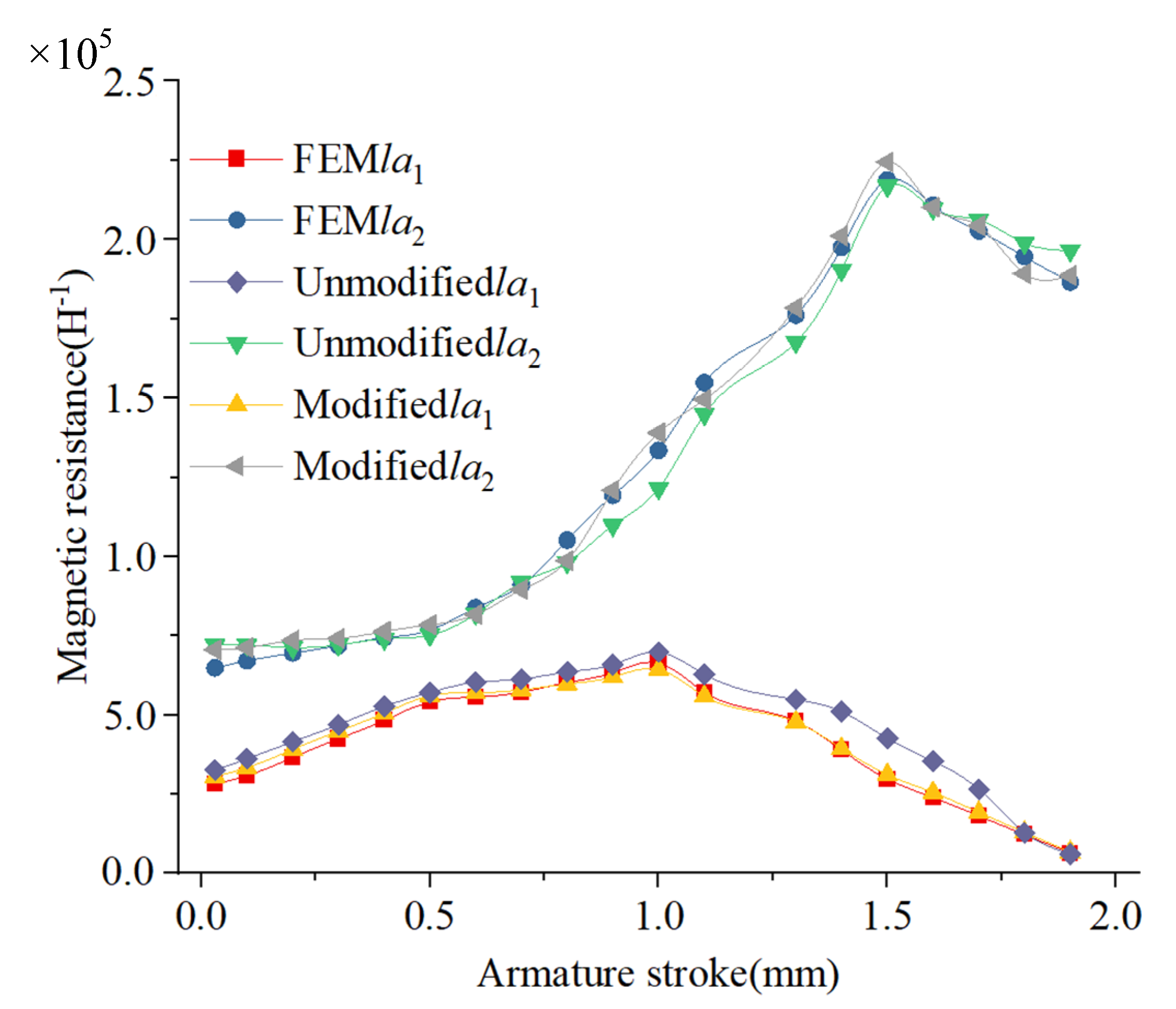
• The proposed method can effectively improve the calculation accuracy of the solenoid valve electromagnetic system. Compared with the FEM data, the unmodified MFL permeance of the DPM mean error is 13.1%, and the modified MFL permeance of the DPM mean error is 4.7%. The unmodified MFL permeance of the DPM mean error is 9.94%, and the modified MFL permeance of the DPM mean error is 3.7%.
• The results of the DPM solenoid valve electromagnetic system in the case study showed a significant improvement. Particularly, the calculation accuracy improved by reducing the DPM mean error from 10.2% to 3.8%.

References

1. Hong, D.K.; Woo, B.C.; Koo, D.H.; Lee, K.C. Electromagnet Weight Reduction in a Magnetic Levitation System for Contactless Delivery Applications. Sensors 2010, 10, 6718–6729. [Google Scholar] [CrossRef] [PubMed]
2. Yang, X.M.; Guo, X.L.; Ouyang, H.J.; Li, D.S. A Kriging Model Based Finite Element Model Updating Method for Damage Detection. Appl. Sci. 2017, 7, 1039. [Google Scholar] [CrossRef] [Green Version]
3. Zhang, X.X.; Liu, G.D.; Wang, K.T.; Li, X.D. Application of a Hybrid Interpolation Method Based on Support Vector Machine in the Precipitation Spatial Interpolation of Basins. Water 2017, 9, 760. [Google Scholar] [CrossRef] [Green Version]
4. Zhang, D.W.; Li, W.L.; Wu, X.H.; Liu, T. An Efficient Regional Sensitivity Analysis Method Based on Failure Probability with Hybrid Uncertainty. Energies 2018, 11, 1684. [Google Scholar] [CrossRef] [Green Version]
5. Li, Y.K.; Song, B.W.; Mao, Z.Y.; Tian, W.L. Analysis and Optimization of the Electromagnetic Performance of a Novel Stator Modular Ring Drive Thruster Motor. Energies 2018, 11, 1598. [Google Scholar] [CrossRef] [Green Version]
6. Kwon, J.W.; Lee, J.H.; Zhao, W.L.; Kwon, B.I. Flux-Switching Permanent Magnet Machine with Phase-Group Concentrated-Coil Windings and Cogging Torque Reduction Technique. Energies 2018, 11, 2758. [Google Scholar] [CrossRef] [Green Version]
7. You, Y.M. Multi-Objective Optimal Design of Permanent Magnet Synchronous Motor for Electric Vehicle Based on Deep Learning. Appl. Sci. 2020, 10, 482. [Google Scholar] [CrossRef] [Green Version]
8. Pan, R.C.; Song, Z.Y.; Liu, B. Optimization Design and Analysis of Supersonic Tandem Rotor Blades. Energies 2020, 13, 3228. [Google Scholar] [CrossRef]
9. Bae, T.S.; Lee, K.H. Structural Design of a Main Starting Valve Based on the First Axiom. Int. J. Precis. Eng. Manuf. 2012, 13, 685–691. [Google Scholar] [CrossRef]
10. Lee, Y.M.; Choi, D.H. Design Optimization of an Automotive Vent Valve Using Kriging Models. Trans. KSAE 2011, 16, 1–9. [Google Scholar]
11. Kim, S.P.; Lee, K.H. Structural Optimization of a Manifold Valve for Pressure Vessel. J. Korean Soc. Precis. Eng. 2009, 26, 102–109. [Google Scholar]
12. Xue, X.F.; Wang, Y.Z.; Lu, C.; Zhang, Y.P. Sinking Velocity Impact-Analysis for the Carrier-Based Aircraft Using the Response Surface Method-Based Improved Kriging Algorithm. Adv. Mater. Sci. Eng. 2020, 6, 1–13. [Google Scholar] [CrossRef]
13. Rashki, M.; Azarkish, H.; Rostamian, M.; Bahrpeyma, A. Classification Correction of Polynomial Response Surface Methods for Accurate Reliability Estimation. Struct. Saf. 2019, 81, 101869. [Google Scholar] [CrossRef]
14. Sumiya, U.; Kwon, H.H. Development of bias correction scheme for high resolution precipitation forecast. J. Korea Water Resour. Assoc. 2018, 51, 575–584. [Google Scholar]
15. Wang, X.; Babovic, V.; Li, X. Application of Spatial-Temporal Error Correction in Updating Hydrodynamic Model. J. Hydro Environ. Res. 2017, 16, 45–57. [Google Scholar] [CrossRef]
16. Rathore, P.; Kumar, D.; Rajasegarar, S.; Palaniswami, M. Maximum Entropy-Based Auto Drift Correction Using High-and Low-Precision Sensors. ACM Trans. Sens. Netw. 2017, 13, 1–41. [Google Scholar] [CrossRef]
17. Alexeeff, S.E.; Carroll, R.J.; Coull, B. Spatial measurement error and correction by spatial SIMEX in linear regression models when using predicted air pollution exposures. Biostatistics 2016, 17, 377–389. [Google Scholar] [CrossRef] [PubMed] [Green Version]
18. Xia, B.; Lee, T.W.; Choi, K.; Koh, C.S. A Novel Adaptive Dynamic Taylor Kriging and Its Application to Optimal Design of Electromagnetic Devices. IEEE Trans. Magn. 2016, 52, 1–4. [Google Scholar] [CrossRef]
19. Zhang, C.; Qang, Z.; Shafieezadeh, A. Value of Information Analysis via Active Learning and Knowledge Sharing in Error-Controlled Adaptive Kriging. IEEE Access 2020, 8, 51021–51034. [Google Scholar] [CrossRef]
20. Chen, D.C.; Liu, D.Z.; Li, Y.H.; Meng, L.; Yang, X.J. Improve Spatiotemporal Kriging with Magnitude and Direction Information in Variogram Construction. Chin. J. Electron. 2016, 25, 527–532. [Google Scholar] [CrossRef]
21. Zhang, J.H.; Xiao, M.; Gao, L.; Zhang, Y. MEAK-MCS: Metamodel Error Measure Function based Active Learning Kriging with Monte Carlo Simulation for Reliability Analysis. In Proceedings of the 2019 IEEE 23rd International Conference on Computer Supported Cooperative Work in Design, Porto, Portugal, 6–8 May 2019. [Google Scholar]
22. Yan, Y.; Wang, J.; Zhang, Y.; Sun, Z. Kriging Model for Time-Dependent Reliability: Accuracy Measure and Efficient Time-Dependent Reliability Analysis Method. IEEE Access 2020, 8, 172362–172378. [Google Scholar] [CrossRef]
23. Liu, X.; Li, X.S.; Huang, S.D. Parameters Optimization of the Permanent Magnet Linear Synchronous Machine Using Kriging-based Genetic Algorithm. In Proceedings of the 2019 22nd International Conference on Electrical Machines and Systems, Harbin, China, 11–14 August 2019. [Google Scholar]
24. Yin, J.; Ng, S.H.; Ming, K. A study on the effects of parameter estimation on kriging model’s prediction error in stochastic simulations. In Proceedings of the 2009 Winter Simulation Conference, Austin, TX, USA, 13–16 December 2009. [Google Scholar]
25. Yu, J.C. Evolutionary algorithm using progressive Kriging model and dynamic reliable region for expensive optimization problems. In Proceedings of the 2016 IEEE International Conference on Systems, Man, and Cybernetics, Budapest, Hungary, 9–12 October 2016. [Google Scholar]
26. Pham, T.D. Kriging-based possibilistic entropy of biosignals. In Proceedings of the 20th European Signal Processing Conference, Bucharest, Romania, 27–31 August 2012. [Google Scholar]
27. Rivera, R. A Low Rank Gaussian Process Prediction Model for Very Large Datasets. In Proceedings of the 2015 IEEE First International Conference on Big Data Computing Service and Applications, Redwood City, CA, USA, 30 March–2 April 2015. [Google Scholar]
28. Jouhaud, J.C.; Sagaut, P.; Labeyrie, B. A kriging approach for CFD/wind-tunnel data comparison. J. Fluids Eng. Trans. ASME 2006, 128, 847–855. [Google Scholar] [CrossRef] [Green Version]
29. Han, S.Q.; Song, W.P.; Han, Z.H. An improved WENO method based on Gauss-kriging reconstruction with an optimized hyper-parameter. J. Comput. Phys. 2020, 422, 109742. [Google Scholar] [CrossRef]
30. Cui, D.; Wang, G.Q.; Lu, Y.P.; Sun, K.K. Reliability design and optimization of the planetary gear by a GA based on the DEM and Kriging model. Reliab. Eng. Syst. Saf. 2020, 203, 107074. [Google Scholar] [CrossRef]
31. Shin, Y.J.; Lee, S.H.; Choi, C.H.; Kim, J.H. Shape Optimization to Minimize The Response Time of Direct-acting Solenoid Valve. J. Magn. 2015, 20, 193–200. [Google Scholar] [CrossRef] [Green Version]
32. Suh, Y.K. Multi-objective Optimization Strategy based on Kriging Metamodel and its Application to Design of Axial Piston Pumps. J. Adv. Mar. Eng. Technol. 2013, 37, 893–904. [Google Scholar]
33. Qin, W.J.; He, J.Q. Optimum design of local cam profile of a valve train. Proc. Inst. Mech. Eng. Part C J. Mech. Eng. Sci. 2010, 224, 2487–2492. [Google Scholar] [CrossRef]
34. Li, T.Z.; Yang, X.L. An efficient uniform design for Kriging-based Response Surface Method and its Application. Comput. Geotechics 2019, 109, 12–22. [Google Scholar] [CrossRef]
35. Trinchero, R.; Larbin, M.; Swaminathan, M.; Canavero, F.G. Statistical Analysis of the Efficiency of an Integrated Voltage Regulator by means of a Machine Learning Model Coupled with Kriging Regression. In Proceedings of the IEEE Workshop on Signal and Power Integrity, Chambery, France, 18–21 June 2019. [Google Scholar]
36. Liang, H.M.; Zhang, K.; You, J.X. Analytical Method for the Magnetic Field Line Distribution of a Fan-shaped Permanent Magnet and the Calculation of Leakage Permeance. J. Magn. 2017, 22, 395–405. [Google Scholar] [CrossRef]
37. You, J.X.; Zhang, K.; Zhu, Z.W.; Liang, H.M. Novel Design and Research for a High-retaining-force, Bi-directional, Electromagnetic Valve Actuator with Double-layer Permanent Magnets. J. Magn. 2016, 21, 65–71. [Google Scholar] [CrossRef]
38. Zhang, K.; Liang, H.M.; You, J.X.; Yu, H. Distributed Parameter Model for Electromagnetic Valve Actuator with Permanent Magnet. In Proceedings of the IEEE International Magnetics Conference, Dublin, Ireland, 24–28 April 2017. [Google Scholar]
39. Ye, X.R.; Chen, H.; Liang, H.M.; Chen, X.J.; You, J.X. Multi-Objective Optimization Design for Electromagnetic Devices with Permanent Magnet Based on Approximation Model and Distributed Cooperative Particle Swarm Optimization Algorithm. IEEE Trans. Magn. 2018, 54, 1–5. [Google Scholar]
40. Ye, X.R.; Chen, H.; Chen, C.; Zhai, G.F. Life-cycle Dynamic Robust Design Optimization for Batch Production of Permanent Magnet Actuator. IEEE Trans. Ind. Electron. 2020, 11, 3026294. [Google Scholar] [CrossRef]
Figure 1. Solenoid valve with fan-shaped permanent magnet (PM): (a) sectional view of solenoid valve; (b) magnetic flux tube diagram (half of Figure 1a).
Actuators 10 00010 g001
Figure 2. The leakage permeance of FEM and before error modifying the distributed parameter model.
Actuators 10 00010 g002
Figure 3. The leakage permeance error values in 0 AT.
Actuators 10 00010 g003
Figure 4. The comparison of ΔG3 calculations and FEM data on basis functions.
Actuators 10 00010 g004
Figure 5. The basis function of Gaussian error data fitting.
Actuators 10 00010 g005
Figure 6. Standard Schwefel function.
Actuators 10 00010 g006
Figure 7. Schwefel function and ΔG3, ΔG4 curves.
Actuators 10 00010 g007
Figure 8. The leakage permeance of FEM and error modified distributed parameter model (DPM).
Actuators 10 00010 g008
Figure 9. The soft magnetic resistance of FEM and unmodified and modified DPM.
Actuators 10 00010 g009
Figure 10. FEM and unmodified and modified DPM force data on the armature.
Actuators 10 00010 g010
Figure 11. Flow chart of method for DPM based on kriging basis function predictive identification program (PIP) error correction.
Actuators 10 00010 g011