Real-Time Anti-Saturation Flow Optimization Algorithm of the Redundant Hydraulic Manipulator

Abstract

As a typical single-pump multi-actuator system, the hydraulic manipulator faces the flow saturation problem when moving at a high speed to track a desired trajectory. To overcome this problem, this paper proposes a real-time anti-saturation flow optimization algorithm based on the gradient projection method. By projecting the gradient of the demand flow in the null space of the task Jacobians, this algorithm can reduce the flow demand while enforcing a global volumetric flow limit in real time. The model of a 7-degree-of-freedom (DOF) hydraulic redundant manipulator was established to carry out theoretical derivation and algorithm design. Then, the experimental verification was completed on the real manipulator platform. Experimental results show that this algorithm reduces average demand flow by 9.85% and average power consumption by 310.3 W under no saturation condition. When flow saturation occurs, the algorithm can increase the average endpoint velocity by 7.52% and reduce the maximum directional error by 71.73% with an average calculation time step of 3 ms. The average trajectory position error can also be reduced by 42.59% compared with the anti-saturation algorithm. Therefore, the proposed algorithm can achieve real-time optimization to reduce flow consumption and achieve anti-saturation in practical applications of redundant hydraulic manipulator.

1. Introduction

Hydraulic manipulators have been used for decades in a variety of areas (e.g., construction, mining, and forestry) due to their larger power-to-weight ratio and higher robustness compared with electric manipulators (e.g., industrial robots) [1]. However, in contrast with electric manipulators with a high level of automation, most commercial hydraulic manipulators (e.g., excavators) still use traditional manual operation, which needs a human to operate each hydraulic actuator separately to control the end-effector velocity so that it requires high proficiency of the operator. Therefore, the industry and academia areas have been committed to the research on the coordinated control of hydraulic manipulators to directly guide the end-effector trajectory [2,3,4], which means that the inverse kinematic relationship should be established between the joint space and task space.

However, general inverse solutions used for industrial robots are designed [5,6,7] without considering the flow constraint of the hydraulic manipulators [8,9], which will lead to flow saturation that the demand flow exceeds the maximum flow provided by the system in practical applications. At this point, the least loaded actuator will receive the flow primarily, while the most loaded actuator cannot track the desired trajectory, resulting in undesired motion of the end-effector. This is a very dangerous condition for a heavy-duty manipulator, which may cause serious safety incidents and should be avoided to the utmost. Consequently, the commercial solutions generally set the velocity of the end-effector to a small enough value so that no operation will cause the flow limit to be exceeded, but a large motion potential cannot be exploited since the maneuverability varies dramatically in different manipulator configurations [10]. For this reason, Lampinen et al. [11] proposed an on-line trajectory scaling method considering the volumetric flow limit. Essentially, the method always maintains achievable velocity according to the maximum supply flow of the system. Similar velocity scaling algorithms are also mentioned in the literature [12,13]. They all use a scaling factor to reduce the velocity of the end-effector so that the flow is limited within the boundary before flow saturation occurs. Compared with commercial solutions, these algorithms improve efficiency while ensuring tracking accuracy. However, one problem is that none of them reduces the demand flow during the movement of the manipulator.

Due to the complexity of operation in an unstructured environment, the general hydraulic manipulators are equipped with redundant joints. Accordingly, in the process of executing the same trajectory-tracking task, the velocity distribution of each joint can be different, which leaves room for further improvements in the manipulator’s work efficiency. Referring to the methods of electric manipulators using redundant joints for motion planning [14,15,16,17,18], there is also some related research on hydraulic manipulators. For example, Ortiz Morales et al. [19] addressed the joint-limited minimum-time redundancy resolution of hydraulic manipulators, and Löfgren [20] studied redundancy resolution, which maximizes load capacity. In addition, Beiner et al. [21] proposed a pseudo-inverse method for redundancy resolution to minimize the cylinder velocity norm in the hydraulic manipulator’s actuator space. Nurmi et al. [22,23] derived an algorithm using dynamic programming for global energy optimization of a redundant manipulator. Nevertheless, to the best of the author’s knowledge, an algorithm aimed at reducing the demand flow during the movement of redundant manipulators has not been addressed in the existing literature. Although the minimum energy is equivalent to the minimum flow in a constant pressure system, the application of dynamic programming is limited in unstructured environments, which need real-time trajectory generation.

Therefore, this paper proposes a real-time anti-saturation flow optimization algorithm based on gradient projection method, which can reduce the demand flow without affecting the endpoint velocity of the manipulator. Compared with the existing anti-saturation algorithm, our approach can further improve the operating efficiency of the manipulators while reducing energy consumption. Furthermore, the algorithm can be applied to actual human operation due to its real-time performance. In this paper, a 7-degree-of-freedom (DOF) hydraulic redundant manipulator was used as an example to carry out theoretical derivation and algorithm design, and finally, the experimental verification was completed on the real manipulator platform.

2. Model of Hydraulic Manipulator

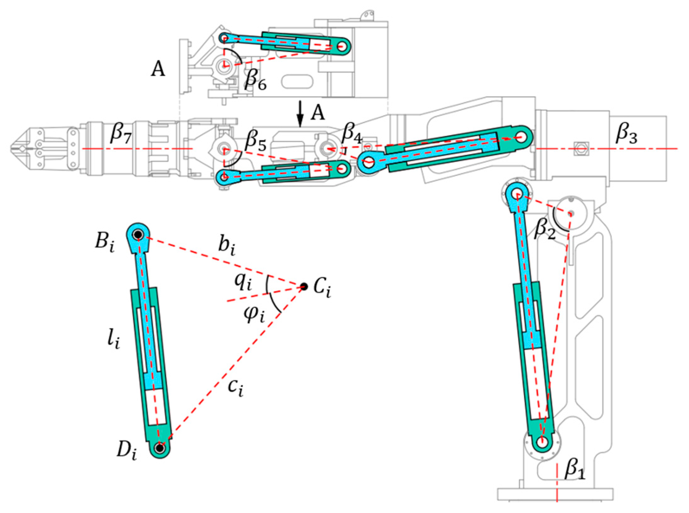
2.1. Forward Kinematics Model

The structure of the 7-DOF hydraulic manipulator studied in this paper is shown in Figure 1. Its shoulder yaw, arm roll, and wrist roll joints are driven by swing cylinders, while the arm pitch, elbow pitch, wrist pitch, and wrist yaw joints are driven by linear cylinders. The standard Denavit–Hartenberg (D–H) parameter method [24] is used to establish the forward kinematics model of the manipulator. The D–H parameters of the model are shown in

Table 1. The D–H parameters of manipulator.

Joint Number	${\mathit{\theta }}_{\mathit{i}}(°)$	${\mathit{d}}_{\mathit{i}}\left(\mathit{m}\mathit{m}\right)$	${\mathit{a}}_{\mathit{i}}\left(\mathit{m}\mathit{m}\right)$	${\mathit{\alpha }}_{\mathit{i}}(°)$	$\mathbf{Joint} \mathbf{Limit} (°)$	Joint Name
1	$q_1$− 90	1015	55	−90	[−45, 45]	Should yaw
2	$q_{2 }$− 90	0	225	90	[−60, 40]	Arm pitch
3	$q_3$	846	0	−90	[−45, 45]	Arm roll
4	$q_4$− 90	0	360	0	[0, 120]	Elbow pitch
5	$q_5$	0	0	−90	[−40, 40]	Wrist pitch
6	$q_6$+ 90	464	0	90	[−40, 40]	Wrist yaw
7	$q_7$	277	0	0	[−135, 135]	Wrist roll

, and the corresponding D–H coordinate system is shown in Figure 2 (the configuration of the manipulator shown in Figure 2 is the joint null position).

In Table 1, ${\theta }_i, d_i$, $a_i$, ${\alpha }_i$ and $q_i$ denote the joint angle, link offset, link length, link twist, and joint position, respectively (a nomenclature section is given in Appendix A). Then the homogeneous transformation from the link coordinate frame to the coordinate frame {i} can be expressed as:

$$A_{i-1}^i\left({\theta }_i,d_i,a_i,{\alpha }_i\right)=T_{Rz}\left({\theta }_i\right)T_z\left(d_i\right)T_x\left(a_i\right)T_{Rx}\left({\alpha }_i\right),$$

(1)

It can be expanded into:

$$A_{i-1}^i=\left[\begin{array}{cccc}\cos {\theta }_i& -\sin {\theta }_i\cos {\alpha }_i& \sin {\theta }_i\sin {\alpha }_i& a_i\cos {\theta }_i\\ \sin {\theta }_i& \cos {\theta }_i\cos {\alpha }_i& -\cos {\theta }_i\sin {\alpha }_i& a_i\sin {\theta }_i\\ 0& \sin {\alpha }_i& \cos {\alpha }_i& d_i\\ 0& 0& 0& 1\end{array}\right].$$

(2)

Therefore, the homogeneous transformation of the endpoint coordinate frame relative to the base coordinate frame is:

$$T_0^7=A_0^1{A}_1^2{A}_2^3{A}_3^4{A}_4^5{A}_5^6{A}_6^7,$$

(3)

2.2. Hydraulic Cylinder Driving Model

Each joint of the manipulator is driven by a hydraulic cylinder. To control the trajectory of the endpoint, it is necessary to establish the movement relationship between each joint and its driving mechanism. In this manipulator, the 2nd, 4th, 5th, and 6th joints are all driven by a single-rod linear cylinder, and the driving mechanism is a typical rotating guide-bar mechanism, as shown in Figure 3.

In Figure 3, the unified model representation of four joint drive mechanisms is presented in the lower left corner. Point $C_i$ represents the hinge point between link i and link i + 1. Point $D_i$ denotes the hinge point between the drive hydraulic cylinder and link i, and point $B_i$ represents the hinge point between the other end of the hydraulic cylinder and link i + 1. The lengths of the segments $C_i{B}_i$ and $C_i{D}_i$ are $b_i$ and $c_i$, respectively. The angle between the segment $C_i{B}_i$ and $C_i{D}_i$ is ${\beta }_i$, and ${\beta }_i$ is the sum of joint position $q_i$ and joint offset ${\phi }_i$ (for the joints driven by the swing cylinder, ${\beta }_i$ is the swing angle). The relationship between $q_i$ and the total cylinder length $l_i$ can be established according to the law of cosine, which can be expressed as:

$${l_i}^2=b_i^2+c_i^2-2b_i{c}_i\cos {\beta }_i,$$

(4)

Then the joint position can be expressed as:

$$q_i=\arccos \left(\frac{b_i^2+c_i^2-l_i^2}{2b_i{c}_i}\right)-{\phi }_i.$$

(5)

Taking the derivative on both sides of Equation (4), the relationship between cylinder velocity $v_i$ and joint velocity ${\dot{q}}_i$ can be obtained:

$$2l_i{v}_i=2b_i{c}_i\sin \left({\phi }_i+{\theta }_i\right){\dot{q}}_i,$$

(6)

Combining Equations (4) and (6), the equation can be written as:

$$v_i=\frac{b_i{c}_i\sin \left({\phi }_i+{\theta }_i\right)\dot{q_i}}{\sqrt{{b_i}^2+{c_i}^2-2b_i{c}_i\cos \left({\phi }_i+q_i\right)}}={\gamma }_i \left(q_i\right){\dot{q}}_i.$$

(7)

From Equation (7), it can be known that the cylinder velocity $v_i$ is affected by the structural design parameters of the manipulator ($b_i$, $c_i$, ${\phi }_i$), the joint position $q_i$ and the joint velocity ${\dot{q}}_i$.

For the remaining three joints, since they are directly driven by a swing cylinder and the joint offset is 0, their joint position and velocity can be expressed as:

$$q_i={\alpha }_i,$$

(8)

$${\dot{q}}_i={\dot{\alpha }}_i,$$

(9)

In Equations (8) and (9), $q_i$ and ${\dot{q}}_i$ represent the position and velocity of the i-th joint, respectively, and ${\alpha }_i$ and ${\dot{\alpha }}_i$ denote the swing angle and velocity of the i-th swing cylinder, respectively (i = 1, 3, and 7). Combining Equations (7) and (9), the unified expression between the velocity of each joint and the velocity of the hydraulic cylinder is:

$$v_i=f_i \left(q_i\right){\dot{q}}_i,$$

(10)

where:

$$f_i \left(q_i\right)=\{\begin{array}{c}1 , i=1,3,7\\ {\gamma }_i \left(q_i\right) , i=2,4,5,6\end{array}.$$

(11)

3. Anti-Saturation Flow Optimization Algorithm

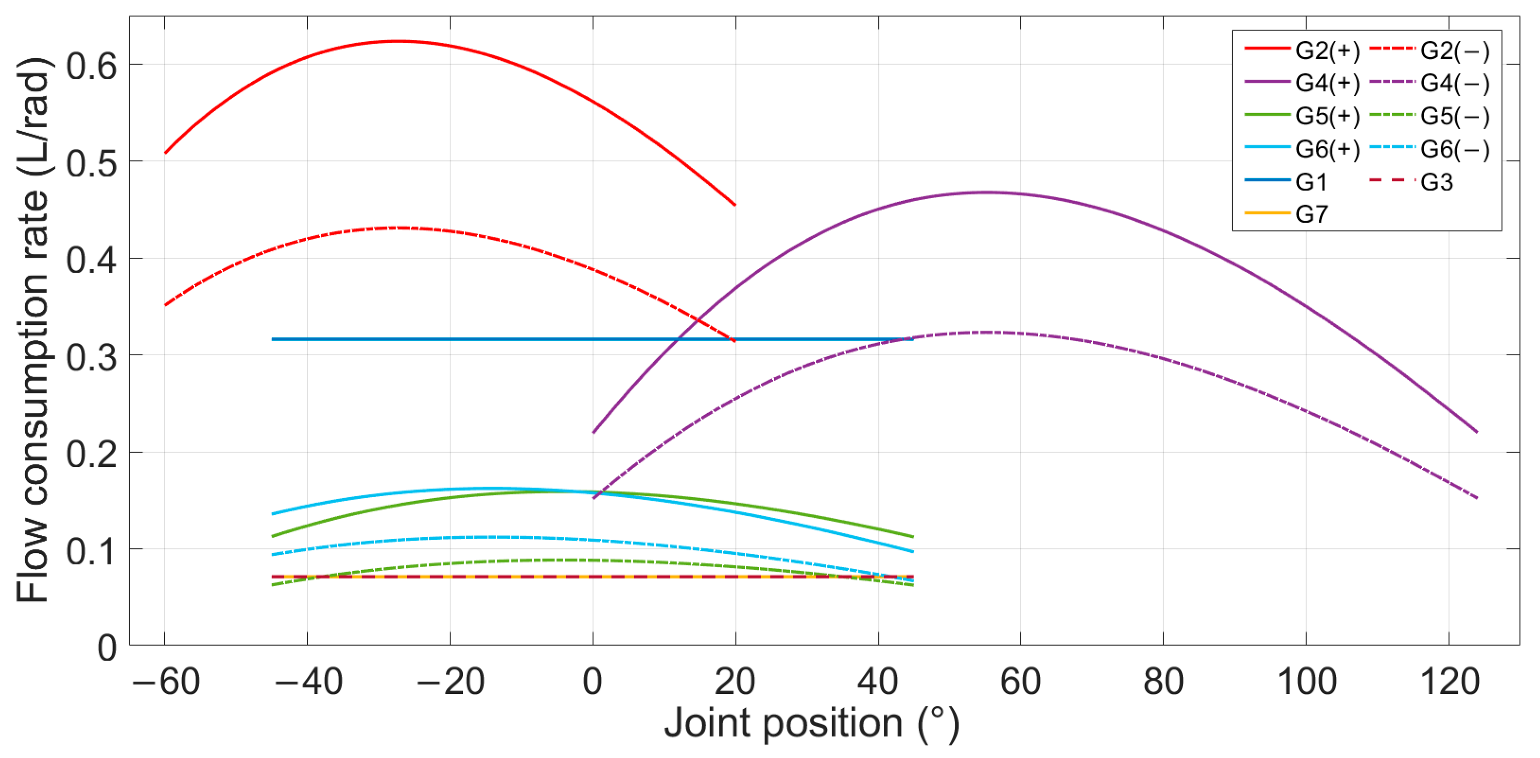
3.1. Inverse Kinematics and Flow Analysis

According to Equations (1) and (3), the forward kinematics equation of the manipulator can be expressed as:

$$\mathit{x}=f\left(\mathit{q}\right).$$

(12)

In Equation (12), $\mathit{x}$ denotes the coordinates of the endpoint in the Cartesian space, and $\mathit{q}$ is the coordinates in the joint space. Taking the derivative on both sides of Equation (12), the relationship between endpoint velocity $\dot{\mathit{x}}$ and joint velocity $\dot{\mathit{q}}$ can be obtained:

$$\dot{\mathit{x}}=J\left(\mathit{q}\right)\dot{\mathit{q}},$$

(13)

where: $J\left(\mathit{q}\right)=\partial f/\partial \mathit{q}$ is the Jacobian matrix of manipulator.

If the endpoint velocity $\dot{\mathit{x}}$ is known, the joint velocity $\dot{\mathit{q}}$ of the manipulator can be obtained by the pseudo-inverse method [25]:

$$\dot{\mathit{q}}=J^{+}\dot{\mathit{x}},$$

(14)

where $J^{+}=J^T{\left(J{J}^T\right)}^{-1}$ is the pseudo-inverse of the Jacobian matrix.

For hydraulic manipulators, the joint space should be further converted into the cylinder space to control the endpoint velocity, and thereby, the hydraulic cylinder driving model of Section 2.2 is used in this chapter.

By observing Equation (7), it can be seen that the joint velocity has a nonlinear relationship with the linear cylinder velocity. In the hydraulic system, the cylinder velocity is related to the flow rate, and its expression is:

$$Q_i=\left|v_i\right|A_i=f_i \left(q_i\right)A_i\left|{\dot{q}}_i\right|,$$

(15)

where $Q_i$ denotes the flow of the i-th hydraulic cylinder, and $A_i$ is the corresponding displacement of the swing cylinder or the effective area of the linear cylinder. The relevant parameters of each joint driving mechanism of the manipulator are shown in

Table 2. The relevant parameters of each joint driving mechanism of the manipulator.

Joint Number	${\mathit{b}}_{\mathit{i}}\left(\mathbf{c}\mathbf{m}\right)$	${\mathit{c}}_{\mathit{i}}\left(\mathbf{c}\mathbf{m}\right)$	${\mathit{\phi }}_{\mathit{i}}(°)$	${\mathit{A}}_{\mathit{i}1}$$\left(\mathbf{c}{\mathbf{m}}^2\right)$	${\mathit{A}}_{\mathit{i}2}$$\left(\mathbf{c}{\mathbf{m}}^2\right)$
1	-	-	0	5.52${ \mathrm{cm}}^3$/° 1
2	20	80.126	102.83	31.172	21.551
3	-	-	0	1.24${ \mathrm{cm}}^3$/°
4	15	67.319	21.95	31.172	21.551
5	10	41.445	80.28	15.904	8.836
6	10.2	41.775	90	15.904	10.996
7	-	-	0	1.24${ \mathrm{cm}}^3$/°

¹ For the swing cylinder, $A_i$ is the effective displacement ($A_i=A_{i1}=A_{i2}$). For the linear cylinder, $A_{i1}$ is the hydraulic cylinder areas without the rod, and $A_{i2}$ is the hydraulic cylinder areas with the rod.

.

According to Equation (15), further analysis shows that when the endpoint velocity is given, different actuators require different flows. For the same actuator, even if the joint velocity is the same, the required flow varies with the change of joint angle and the direction of motion.

In order to express the corresponding relationship between the joint velocity and the actuator flow, the flow consumption rate (FCR) is introduced:

$$G_i=f_i \left(q_i\right) A_i.$$

(16)

The joint’s flow consumption is greater with a greater FCR under the same joint velocity. According to the parameters in

Table 3. PID parameters of each joint in the test.

Joint Number	PID Parameters			Joint Name
	$\mathbf{P}$	$\mathbf{I}$	$\mathbf{D}$
2	$42$	1.07	0	Arm pitch
4	$22$	2.27	0.06	Elbow pitch
5	$19$	0.77	0.2	Wrist pitch

, the FCR of each joint can be drawn with the change of joint angle and motion direction, as shown in Figure 4. In Figure 4, different joints are distinguished by different colors. For the linear cylinders, the negative direction of their movement is the retracting direction of cylinder, which is distinguished by dotted lines.

It can be seen from Figure 4 that Joint 2 has the largest flow consumption, followed by Joint 4, and the FCR of joints 5 and 6 is relatively small and close under the same joint velocity. For these four joints driven by linear cylinders, there is an obvious non-linear relationship between FCR and joint angle.

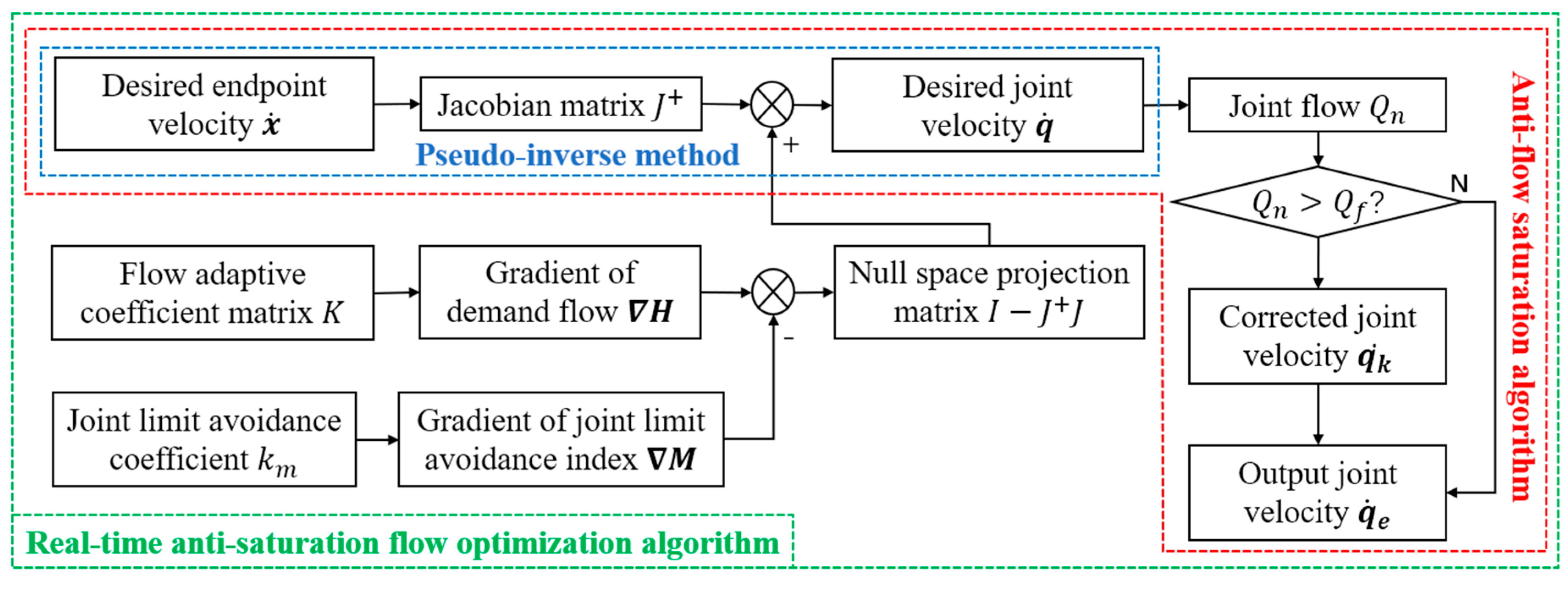
3.2. Anti-Flow Saturation Algorithm

In the single-pump multi-actuator hydraulic system, the maximum supply flow $Q_{max}$ is usually limited by the maximum flow of the pump. When the endpoint moves too fast, flow saturation will occur because the demand flow $Q_d$ is greater than $Q_{max}$. To address this problem, an anti-flow saturation algorithm is used to constrain the demand flow within the maximum supply flow. The demand flow of the system is:

$$Q_d=Q_n+Q_l,$$

(17)

where:

$$Q_n={\displaystyle \sum }_{i=1}^n{Q}_i\left(q_i,{\dot{q}}_i\right),$$

(18)

$Q_l$ is the total leakage flow, and $n$ is the number of joints. According to Equation (15) and Table 2, the flow of the i-th joint can be derived as:

$$Q_i\left(q_i,{\dot{q}}_i\right)=\{\begin{array}{c}{f}_i \left(q_i\right)A_{i1}{\dot{q}}_i ,{\dot{q}}_i\ge 0\\ -f_i \left(q_i\right)A_{i2}{\dot{q}}_i ,{\dot{q}}_i<0\end{array}.$$

(19)

When $Q_d>Q_{max}$, flow saturation occurs. Consequently, the correction coefficient is introduced:

$$k_n=\frac{Q_f}{Q_d-Q_l},$$

(20)

where $Q_f$ is the flow threshold, and its value is slightly less than $Q_{max}$ (it can avoid the impact of fluctuation of supply flow on joint velocity while ensuring a high utilization rate of flow). Then, the corrected joint velocity is:

$$\dot{{\mathit{q}}_k}=k_n\dot{\mathit{q}},$$

(21)

and the system flow after the joint velocity is corrected can be expressed as:

$$Q_{kn}={\displaystyle \sum }_{i=1}^n{Q}_i\left(q_i,{\dot{q}}_k\right)+Q_l.$$

(22)

It can be proved that no matter how large $Q_d$ is, the flow of the system will never exceed $Q_f+Q_l$. The proof is as follows:

$$Q_{kn}={\displaystyle \sum }_{i=1}^n{Q}_i\left(q_i,k_n\dot{q}\right)+Q_l=k_n\left(Q_d-Q_l\right)+Q_l=Q_f+Q_l.$$

(23)

By substituting Equation (19) into Equation (13), the corrected endpoint velocity can be obtained:

$${\dot{\mathit{x}}}_{\mathit{k}}=J\left(\mathit{q}\right){\dot{\mathit{q}}}_{\mathit{k}}=k_n\dot{\mathit{x}}.$$

(24)

According to Equations (17)–(24), the anti-flow saturation algorithm ensures that the demand flow does not exceed the maximum supply flow by decreasing the velocity of each joint in an equal proportion. In this condition, the velocity direction of the endpoint does not change, which will not cause the abrupt change and disorder of the endpoint trajectory. However, the velocity is lower than expected, which will reduce the efficiency of the manipulator.

Furthermore, in some scenarios where the velocity direction is constantly changing (such as master-slave control), the manipulator will have large trajectory errors due to the reduction of velocity, and the error will increase with the increase in velocity error. Therefore, it is necessary to improve the endpoint velocity on the basis of the anti-flow saturation algorithm.

3.3. Anti-Saturation Flow Optimization Algorithm

According to Equations (18) and (22), to increase the endpoint velocity when flow saturation occurs without changing the system hardware, a feasible scheme is to reduce the flow demand of the manipulator. Since the demand flow is mainly determined by the joint velocity, reducing the joint velocity is equivalent to reducing the flow.

The joint velocity obtained by the pseudo-inverse method is the minimum norm solution. However, it can be seen from Figure 4 that the FCR varies greatly with the change of actuators and joint positions, so the smallest joint velocity norm does not mean the smallest flow. Therefore, the gradient projection method can be used to optimize the distribution of joint velocity according to the FCR of the manipulator.

When $\dot{x}$ is given, the general inverse solution can be obtained by solving Equation (13):

$$\dot{\mathit{q}}=\dot{{\mathit{q}}_s}+\dot{{\mathit{q}}_h}=J^{+}\dot{\mathit{x}}+k\left(I-J^{+}J\right)\nabla \mathit{H},$$

(25)

where $\dot{{\mathit{q}}_s}$ is the special solution of Equation (13), which can complete the main task of tracking the given velocity $\dot{x}$, and $\dot{q_h}$ is the projection of the gradient $\nabla H$ of the performance optimization index function in the null space, which can be used to perform some secondary optimization tasks. In addition, $I-J^{+}J$ is the null space projection matrix, and $k$ is the optimization coefficient. The gradient projection method [18] can optimize performance indicators without affecting endpoint velocity by solving Equation (25).

In order to optimize the flow distribution, the demand flow can be used as the objective function to optimize the joint velocity distribution using the gradient projection method. Therefore, according to Section 3.2, the flow optimization performance index can be set as:

$$H={\displaystyle \sum }_{i=1}^n{Q}_i\left(q_i,{\dot{q}}_i\right)+Q_l.$$

(26)

By taking the partial derivative of $H$ for each joint, the gradient $\nabla \mathit{H}$ used for optimization can be obtained. However, the question here is whether to take the partial derivative of the joint position or the joint velocity.

Usually, optimization algorithms take partial derivatives of joint positions, but this is not suitable for flow optimization of hydraulic manipulators. The reason can be easily found by analyzing Figure 4. According to Equations (16), (19), and (26), the partial derivative of the joint position i is:

$$\frac{\partial H}{\partial q_i}=\frac{\partial G_i}{\partial q_i}\left|{\dot{q}}_i\right|.$$

(27)

For the swing cylinder, $G_i$ is a constant, so $\partial H/\partial q_i=0$ has no effect on the velocity of the swing cylinder. For the linear cylinder, $\partial H/\partial q_i$ has a sign change when $G_i$ reaches the maximum value, so $\partial H/\partial q_i$ may increase the joint velocity of a linear cylinder during the movement. Based on the above analysis, taking the partial derivative of the joint velocity may be a more feasible solution. Then, the gradient of $H$ can be written as:

$$\nabla \mathit{H}={\left[\frac{\partial H}{\partial {\dot{q}}_1},\frac{\partial H}{\partial {\dot{q}}_2},\dots ,\frac{\partial H}{\partial {\dot{q}}_n}\right]}^T,$$

(28)

where:

$$\partial H/\partial {\dot{q}}_i=f_i \left(q_i\right)A_i.$$

(29)

According to the gradient projection method, the joint velocity along the direction of $\nabla H$ is the direction that makes the flow increase the fastest. By making k a negative value, this direction can be changed to the direction where the flow decreases fastest. However, when the special solution $\dot{{\mathit{q}}_s}$ obtained from Equation (25) is small, the homogeneous solution $\dot{{\mathit{q}}_h}$ may still be large, which may cause the algorithm fail to achieve flow reduction. For this, the parameter k in Equation (25) is modified to the flow-adaptive coefficient matrix:

$$K=k\bullet diag\left[{\dot{q}}_1,{\dot{q}}_2,\dots ,{\dot{q}}_n\right].$$

(30)

By substituting Equations (28) and (30) into Equation (25), the optimized joint velocity solved by the flow optimization algorithm can be written as:

$${\dot{\mathit{q}}}_o=J^{+}\dot{\mathit{x}}+\left(I-J^{+}J\right)K·\nabla \mathit{H}.$$

(31)

In the actual motion of the manipulator, the workspace of each joint is limited by the mechanical structure, but the gradient projection method does not take this into consideration. In order to prevent the manipulator from exceeding the joint limit, it is also necessary to introduce the joint limit avoidance index:

$$M={\displaystyle \sum }_{i=1}^n\frac{1}{n}\frac{{\left(q_{imax}-q_{imin}\right)}^2}{\left(q_{imax}-q_i\right)\left(q_i-q_{imin}\right)},$$

(32)

where $q_{imax}$ and $q_{imin}$ are the upper limit and the lower limit of the joint position $q_i$, respectively. Its gradient can be expressed as:

$$\nabla \mathit{M}={\left[\frac{\partial M}{\partial q_1},\frac{\partial M}{\partial q_2},\dots ,\frac{\partial M}{\partial q_n}\right]}^T,$$

(33)

where $\partial M/\partial q_i$ is the partial derivative of $M$ with respect to $q_i$, which has a larger value only near the joint limit. Combining Equations (31) and (33), the gradient of avoiding the joint limit avoidance index is also projected into the null space, and the final output joint velocity can be expressed as:

$${\dot{\mathit{q}}}_e=J^{+}\dot{\mathit{x}}+\left(I-J^{+}J\right)\left(K·\nabla \mathit{H}-k_m·\nabla \mathit{M}\right)$$

(34)

where $k_m$ is joint limit avoidance coefficient, and Equation (35) can be proved:

$$\dot{\mathit{x}}=J{\dot{\mathit{q}}}_e=J\left(J^{+}\dot{\mathit{x}}+\left(I-J^{+}J\right)\left(K·\nabla \mathit{H}-k_m·\nabla \mathit{M}\right)\right)=\dot{\mathit{x}}+\left(J-J\right)\left(K·\nabla \mathit{H}-k_m·\nabla \mathit{M}\right),$$

(35)

Therefore, theoretically, the endpoint velocity after optimization is the same as before optimization.

When there is no flow saturation, the application of Equation (34) can reduce the flow demand of the system without affecting the endpoint velocity, and reduce the energy consumption of the system. When flow saturation occurs, the anti-saturation algorithm can be applied after the flow optimization algorithm is applied to increase the velocity of the endpoint. This is the real-time anti-saturation flow optimization algorithm proposed in this article, and its algorithm block diagram is shown in Figure 5.

4. Experimental Verification

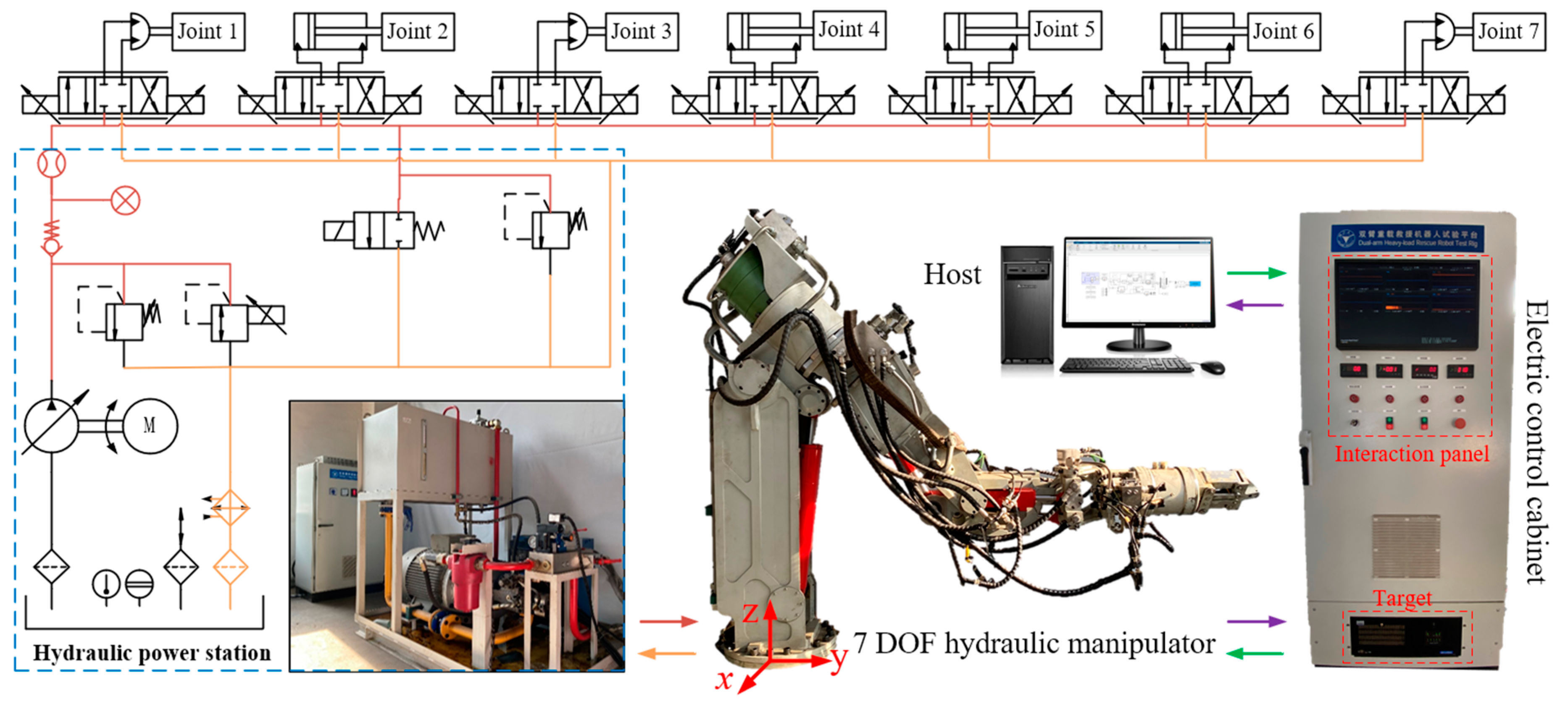
4.1. Introduction of the Experimental Platform

The schematic diagram of the experimental platform of the hydraulic manipulator used in this article for algorithm verification is shown in Figure 6. In Figure 6, the hydraulic system is composed of hydraulic cylinders, servo valves, and a hydraulic power station (HPS). The hydraulic cylinders of each joint are controlled by three-position four-way servo valves and supplied by an electronically controlled pump. The maximum supply flow of the HPS can be set by changing the pump displacement, and the system pressure can be changed by a proportional relief valve. The nominal flow and pressure in the system are 62 L/min and 35 MPa, respectively. A flow meter and a pressure sensor are installed at the outlet of the HPS, which can monitor the system flow and pressure in real time. The control system consists of a host computer, an electrical control cabinet, and sensors. The target computer, servo amplifier and interaction panel are installed in the electric control cabinet, and absolute encoders are installed to obtain joint position and velocity information.

The host computer runs the motion planning algorithm in the Simulink environment, calculates the desired joint position according to the current joint position collected by the target computer, and sends the desired joint position to the target computer by using the user datagram protocol (UDP) communication. The target computer is an industrial computer with a Simulink real-time operating system, which can receive the desired joint position from the host computer and calculate the servo valve control signal by the PID control algorithm (the corresponding PID parameters are shown in Table 3).

In order to avoid different target trajectories in the experiment due to manual operation, which may affect the experimental results, the experimental target trajectory in this article is automatically generated by using the following Equation:

$$\{\begin{array}{c}x\left(t\right)=x_0 \\ y\left(t\right)=y_0+R·\cos \left(\omega t\right)\\ z\left(t\right)=z_0+R·\sin \left(\omega t\right)\end{array},$$

(36)

where t is the algorithm execution time, R is the radius of the target trajectory, ω is the angular velocity of the target trajectory,$\left(x_0, y_0, z_0\right)$ is the coordinates of the circle center, and $\left(x\left(t\right), y\left(t\right), z\left(t\right)\right)$ is the coordinates of the target point at time t.

The desired velocity of the endpoint is generated by the artificial potential field algorithm, and its expression is:

$$\dot{\mathit{x}}\left(t\right)=k_v·\left({\mathit{x}}_t\left(t\right)-{\mathit{x}}_c\left(t\right)\right),$$

(37)

where ${\mathit{x}}_t\left(t\right)$ denotes the coordinates of the target point, ${\mathit{x}}_c\left(t\right)$ represents the coordinates of the endpoint, and $k_v$ is the scaling factor. In the experiment, to improve the maneuverability, the task is to control the endpoint velocity, so the corresponding task’s Jacobian matrix only retained the first three rows of the complete Jacobian matrix.

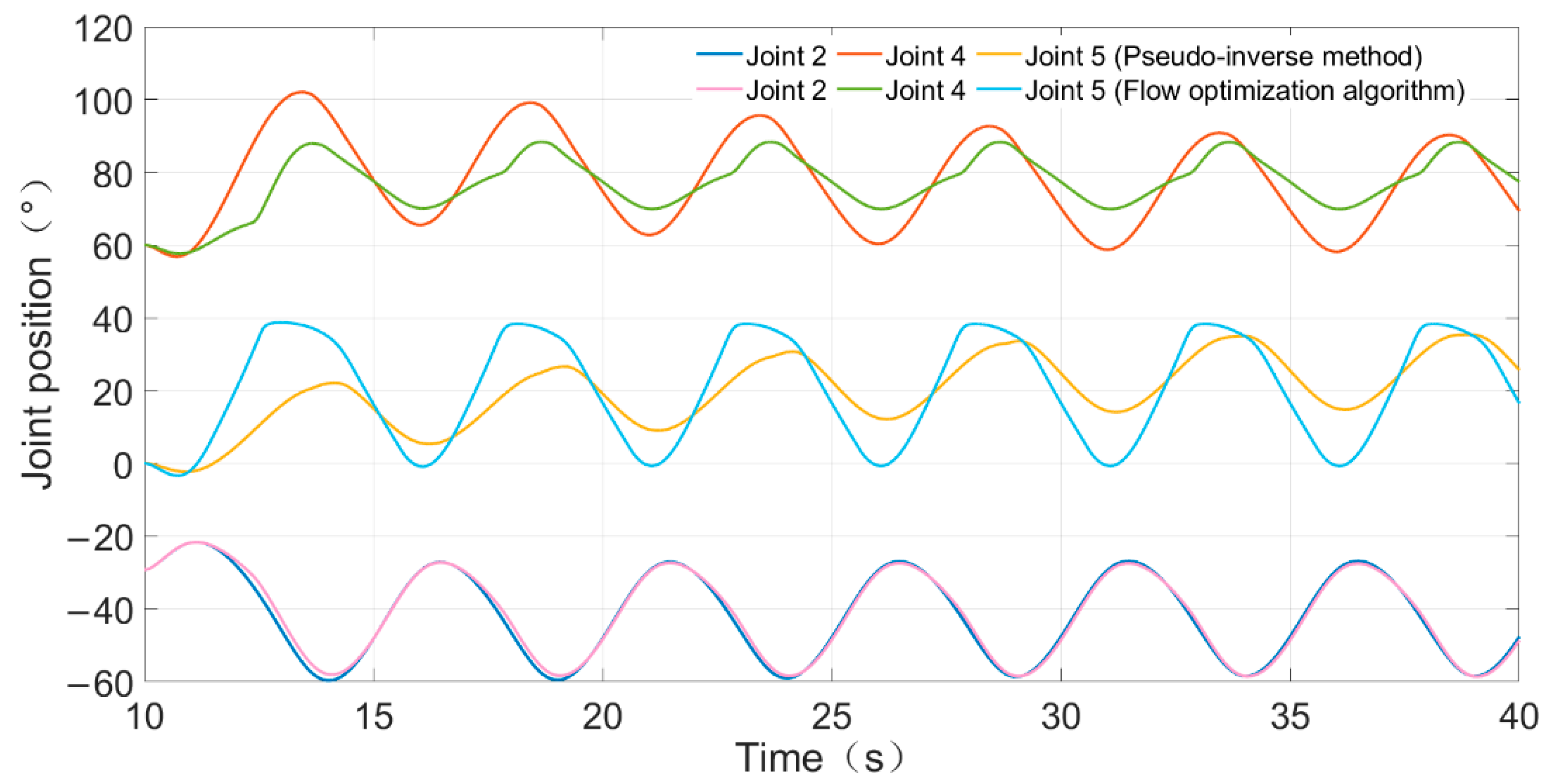
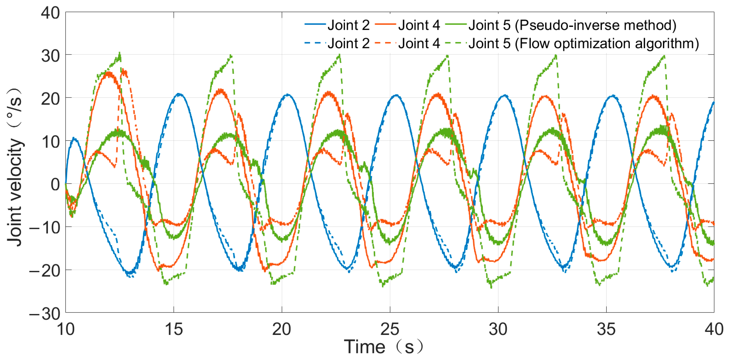
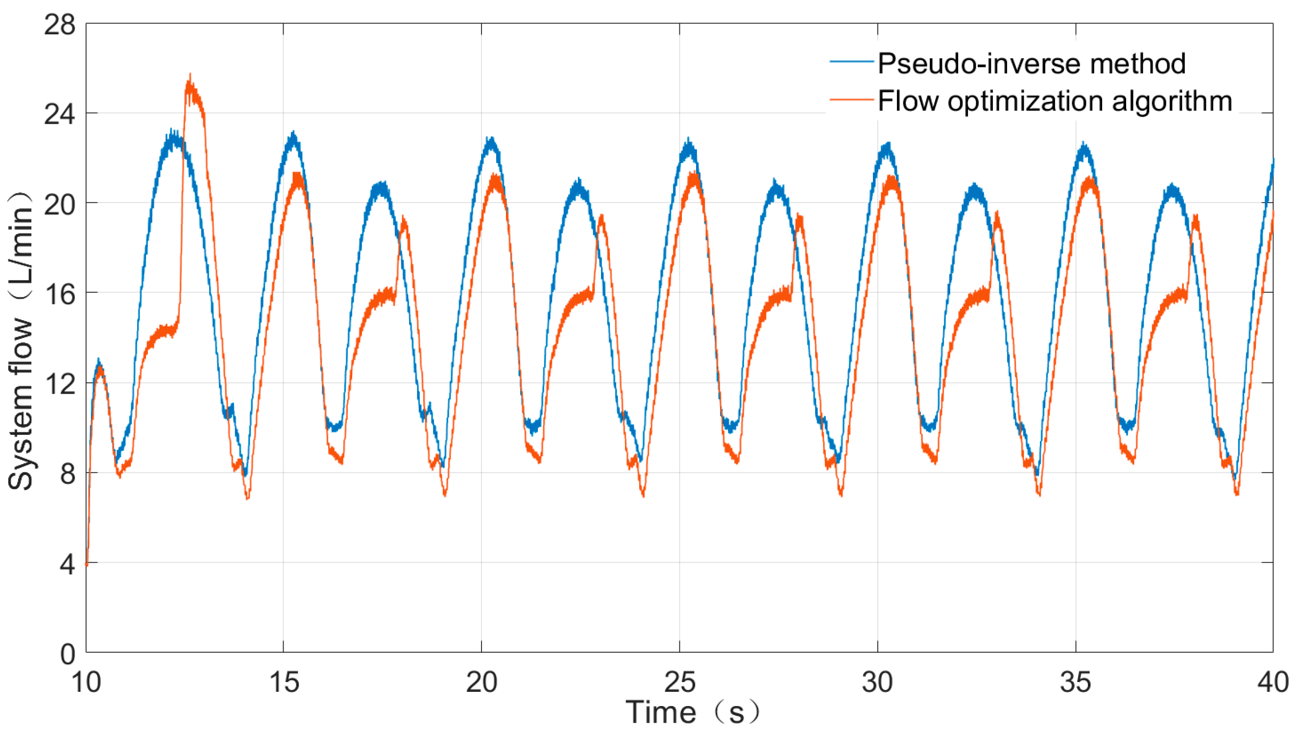
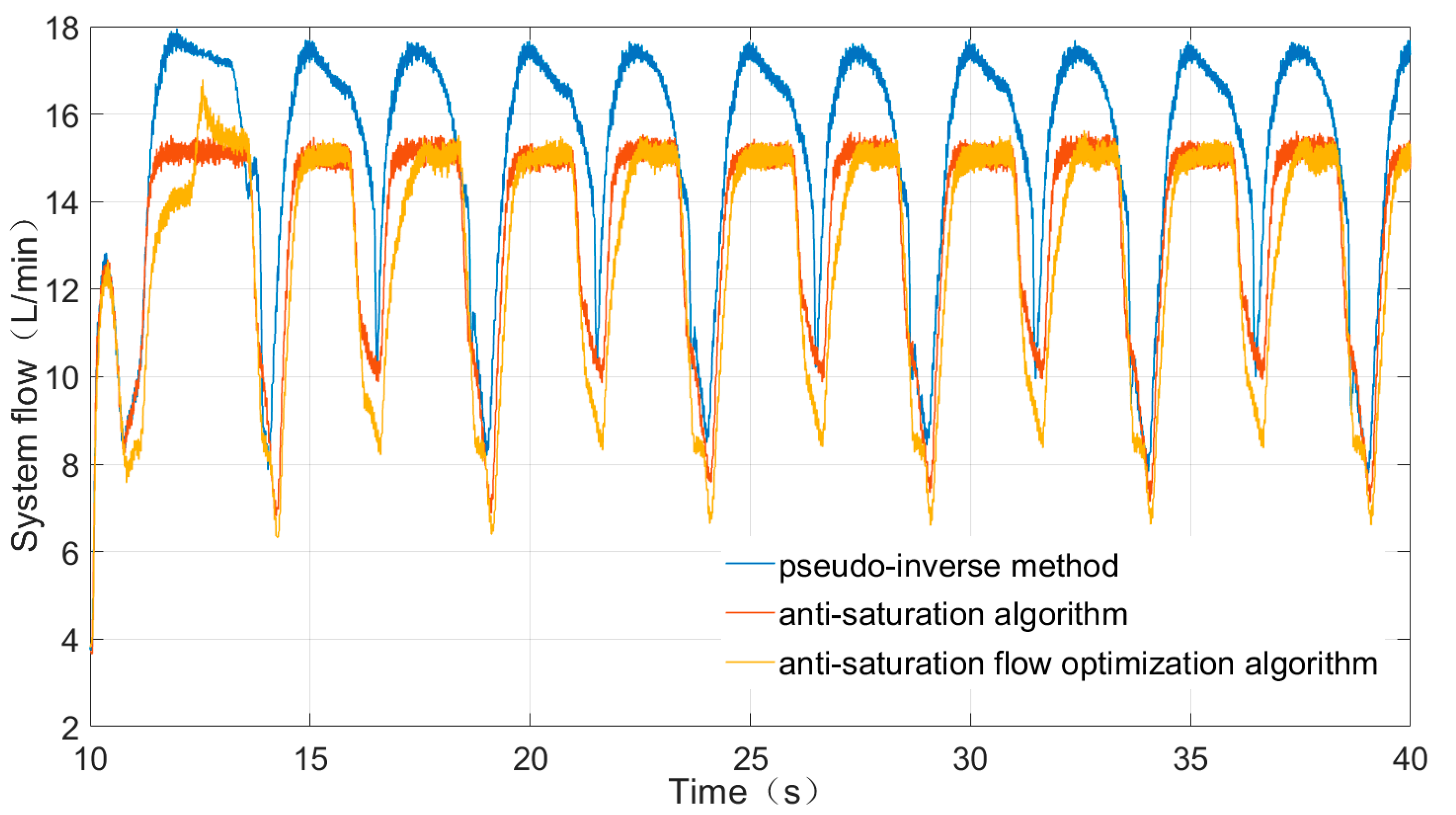
4.2. Experiment for the Flow Optimization Algorithm

In this chapter, the experiments using the pseudo-inverse method and the flow optimization algorithm were carried out separately under the condition of no flow saturation. The joint velocities in the two experiments were calculated by Equations (14) and (34), respectively. For the safety of the experiments, the maximum supply flow of the HPS was set to 26.5 L/min, and the system pressure was set to 12 MPa. Equation (37) was used to calculate the desired velocity of endpoint to track a trajectory described by Equation (36) (where $\left(x_0,y_0,z_0\right)= \left(0, 1.4 \mathrm{m}, 1.4 \mathrm{m}\right), R=0.4 \mathrm{m}, \omega =1.27 \mathrm{rad}/\mathrm{s}$), and the experiment sampling time is 10 ms.

At the beginning of each experiment, the manipulator quickly reached the initial joint coordinates (0°, −30°, 0°, 60°, 0°, 0°, 0°). The experimental algorithm started from $t=10 \mathrm{s}$, and the manipulator stopped moving after 30 s. In each experiment, the joint position, joint velocity, and system flow of the manipulator were recorded. The experimental results are shown in Figure 7, Figure 8, Figure 9 and Figure 10. Substituting the two sets of joint positions collected in the experiment into Equation (3) for forward kinematics calculation, the trajectory of the endpoint in the basic coordinate frame can be found. By plotting the endpoint trajectory in a stable period, a comparison diagram of trajectory is presented in the plane of $x=0$, as shown in Figure 11a. Since only the 2nd, 4th, and 5th joints are used for the motion of the manipulator in the $x=0$ plane, the other joints are not given.

From Figure 7, Figure 8 and Figure 9, it can be seen that the angle variations and velocities of the 2nd and 4th joints using the flow optimization algorithm are reduced compared with those of the pseudo-inverse method. Within 10 s to 40 s, the average actual velocities of Joint 4 in the two experiments are 13.57 °/s and 7.56 °/s, respectively (decreasing 6.01 °/s), while Joint 2 only has a small partial reduction. However, the average velocities of Joint 5 are 7.84 °/s and 15.29 °/s, respectively, with a significant increase of 7.45 °/s. Since the FCR of Joint 5 is much smaller than $G_2$ and $G_4$, the flow consumption of the flow optimization algorithm is dramatically reduced compared with the pseudo-inverse method. According to Figure 8, the theoretical average joint flow of the two experiments can be calculated as 12.654 L/min and 11.120 L/min from Equation (18), respectively (reduced by 12.12%). As shown in Figure 10, from 10 s to 40 s, the average system flow decreases from 15.687 L/min to 14.197 L/min (9.85% reduction). When $t=12.25 \mathrm{s}$, the maximum flow reduction reached about 9.27 L/min. Compared with the theoretical data, the actual flow optimization effect is worse due to the influence of poor dynamic property of hydraulic system [26,27,28]). Nevertheless, it can be seen from Figure 11a that the trajectory of the endpoint was almost unchanged.

Furthermore, in a constant pressure system that does not consider pressure and flow loss, energy consumption can be calculated by the following formula:

$$E_c=\underset{t_1}{\overset{t_2}{\int }}pQ\left(t\right)dt,$$

(38)

where $t_1$ and $t_2$ are the start and end time respectively, $p$ represents the system pressure (12 MPa in this article), $Q\left(t\right)$ is the volumetric flow function. Then, substituting the cumulative flow of the two experiments into Equation (38), it can be calculated that the energy consumptions from 10 s to 40 s are 94.490 kJ and 85.182 kJ, respectively, and it reduced average power consumption by about 310.3 W (9.85%) under no saturation condition.

In the experiments, when Joint 5 was close to the joint limit, its velocity decreased rapidly due to the influence of the joint limit. At that time, the velocity of Joint 4 suddenly increased to ensure that the velocity of endpoint was not affected, which caused the flow to spike. Because the algorithm did not consider the dynamic model for the time being, the abrupt change of velocity also resulted in the local error between the two experimental trajectories.

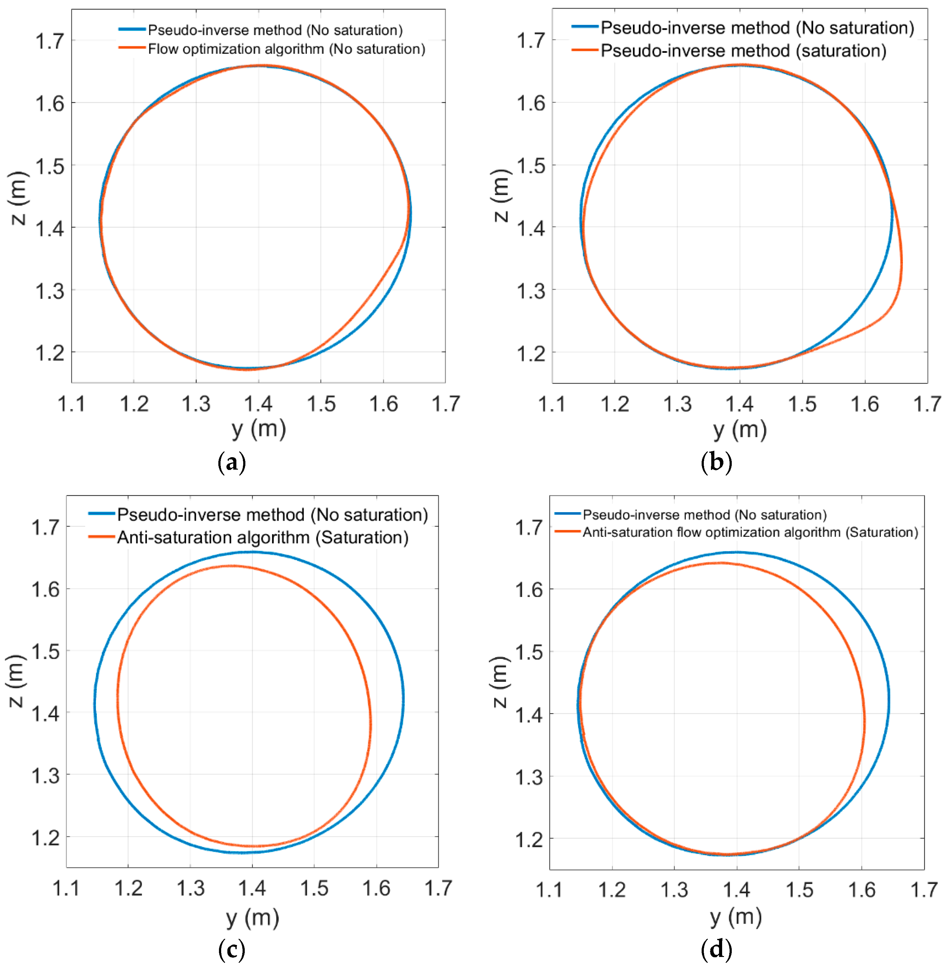
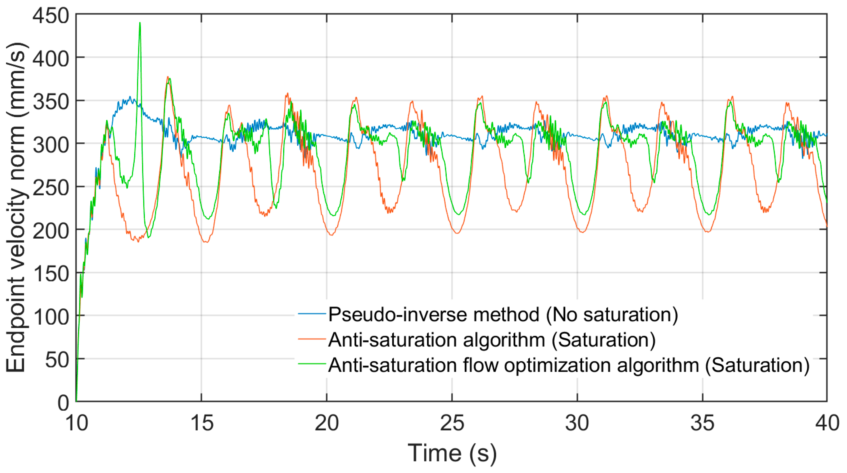
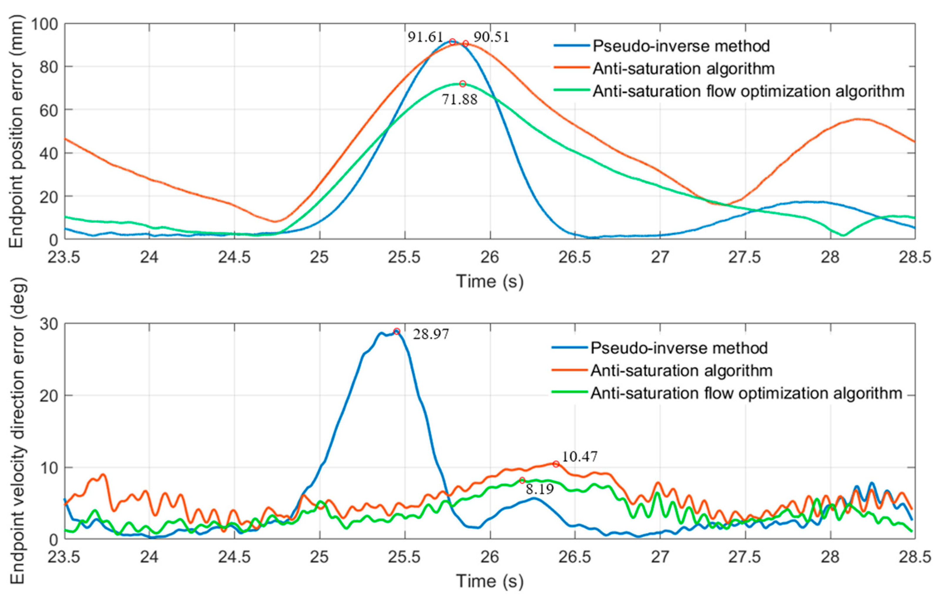
4.3. Anti-Saturation Flow Optimization Algorithm Experiment

The anti-saturation flow optimization algorithm experiment was carried out under the condition of flow saturation, and the maximum supply flow of the HPS was set to 17 L/min. The experiment was carried out three times in total, including the pseudo-inverse method experiment, the anti-saturation algorithm experiment, and the anti-saturation flow optimization algorithm experiment. The joint velocity of the manipulator was calculated by Equations (14), (21), and (34). In addition, the flow threshold in the experiment was set to 15 L/min. Other experimental conditions were the same as the flow optimization algorithm experiment. The comparison diagram of the endpoint trajectory in a same stable period is shown in Figure 11b–d, and the comparison diagram of the system flow in the three experiments is shown in Figure 12. In addition, the endpoint velocity can be obtained by differentiating the trajectories, and the comparison diagram of the endpoint velocity after mean filtering using three algorithms is shown in Figure 13. According to the trajectories in Figure 11, the endpoint position error and velocity direction error of the trajectories of the three algorithms can be calculated when flow saturation occurs, which is shown in Figure 14.

It can be seen from Figure 12 that the system flow peak of the pseudo-inverse method is limited by the maximum supply flow and cannot reach 23.5 L/min (where there is no flow saturation). Therefore, flow saturation occurs at that time, and the lower right corner of the corresponding trajectory clearly deviates from the normal trajectory (as shown in Figure 11b). Figure 14 shows that the maximum position error of the pseudo-inverse method at saturation reaches 91.61 mm. In addition, the endpoint velocity direction (along the tangent of the trajectory) also deviates significantly from the normal direction, and the maximum velocity direction error reaches 28.97° (as shown in Figure 14). If there are obstacles outside the normal trajectory, it may cause some serious accidents.

The anti-saturation algorithm limits the system flow within the maximum flow by reducing the endpoint velocity to avoid flow saturation, and its trajectory is shown in Figure 11c. However, it can be seen from Figure 11c that the trajectory size is clearly reduced due to the decrease in the endpoint velocity, and it can be calculated from Figure 14 that the maximum error and average error of its endpoint position are 90.51 mm and 42.83 mm, respectively. This is because the anti-saturation algorithm reduces the average velocity of the endpoint from the original value 308.05 mm/s to 267.48 mm/s from 10 s to 40 s.

When the anti-saturation flow optimization algorithm is applied, the system flow is still limited within the maximum flow, but the average endpoint velocity increased to 287.60 mm/s (an increase of 20.12 mm/s, about 7.52%) because the algorithm reduces the flow demand of the system. Therefore, the trajectory size is obviously increased compared to the anti-saturation algorithm in Figure 11d, which is also closer to the normal one. It can be seen from Figure 14 that the maximum endpoint velocity direction error of the anti-saturation flow optimization algorithm is 8.19° (reduced by 71.73% compared with the pseudo-inverse method), and the maximum error and average error of its endpoint position are 71.88 mm and 24.59 mm, respectively (reduced by 20.58% and 42.59% compared with the anti-saturation algorithm). As the extent of flow saturation increases, it is predicted that the optimization effect will be more significant.

Substituting the cumulative flow measured in experiments using the anti-saturation algorithm (6677.3 mL) and anti-saturation flow optimization algorithm 6386.9 mL) into Equation (38), the corresponding energy consumptions are calculated as 80.128 kJ and 76.643 kJ, respectively. The data show that the anti-saturation flow optimization algorithm can only reduce energy consumption by 4.37%, which is due to flow saturation during the experiment. Compared with the energy consumption reduction in Section 4.2, the anti-saturation flow optimization algorithm has a better energy-saving effect when there is no flow saturation.

In addition, for the dynamic programming algorithm [23], a complete calculation of a working cycle is required before execution, and the calculation is time-consuming (about 20 min for the same desired trajectory given in Equation (35)). In contrast, our algorithm can achieve real-time calculations with an average time step of 3 ms on our computer (with an Intel Core i7 processor, 2.6 GHz). This is quite critical in practical applications because most hydraulic manipulators require real-time operation under unstructured environments.

Therefore, it can be concluded that the anti-saturation flow optimization algorithm can effectively improve the work efficiency and reduce the trajectory tracking error in real time when the flow saturation occurs.

5. Conclusions

When the flow saturation occurs, the turbulence of the working trajectory will affect the normal operation of the manipulator and even cause serious accidents. The traditional anti-flow saturation algorithm only restricts the flow within the maximum flow of the system by reducing the operating velocity but does not further optimize the flow distribution. To solve this problem, this article proposes a real-time anti-saturation flow optimization algorithm based on the gradient projection method. By projecting the gradient of the demand flow in the null space of the task Jacobians, the flow demand can be reduced significantly without affecting the endpoint velocity performance in real time. Furthermore, when flow saturation occurs, the endpoint velocity can be further improved.

Experimental results show that this algorithm reduces the average demand flow and energy consumption by 9.85% under no saturation conditions. When flow saturation occurs, the algorithm can reduce the maximum directional error by 71.73% compared with pseudo-inverse method. Meanwhile, compared with the anti-saturation algorithm, it can increase the average endpoint velocity by 7.52% and reduce the average track position error by 42.59% and the maximum track position error by 20.58%. Moreover, the algorithm can always ensure good real-time performance during execution (the average time step is 3 ms).

Since the load of hydraulic manipulators is usually much greater than that of electric manipulators, the algorithm proposed in this paper needs to consider the dynamic model to obtain better motion performance in practice. Moreover, since the gradient projection method can also handle multi-priority tasks, the performance of the manipulator can be further improved by adding other objective functions (for example, obstacle constraints and acceleration constraints) based on the algorithm proposed in this paper. These are the works we are committed to in the future.

References

1. Mattila, J.; Koivumaki, J.; Caldwell, D.G.; Semini, C. A Survey on Control of Hydraulic Robotic Manipulators with Projection to Future Trends. IEEE ASME Trans. Mechatron. 2017, 22, 669–680. [Google Scholar] [CrossRef]
2. Deere, J. Intelligent Boom Control Ibc. Available online: https://www.deere.co.uk/en/forestry/ibc/ (accessed on 20 November 2020).
3. HIAB CONTROL SYSTEMS. Available online: https://www.hiab.com/en/products/loader-cranes/hiab-control-systems (accessed on 20 November 2020).
4. Technion. Technion Xcrane Crane Control System. Available online: https://technion.fi/wp-content/uploads/xcrane-brochure-en.pdf (accessed on 20 November 2020).
5. Faroni, M.; Beschi, M.; Pedrocchi, N. Inverse Kinematics of Redundant Manipulators with Dynamic Bounds on Joint Movements. IEEE Robot. Autom. Lett. 2020, 5, 6435–6442. [Google Scholar] [CrossRef]
6. Woolfrey, J.; Lu, W.J.; Liu, D.K. A Control Method for Joint Torque Minimization of Redundant Manipulators Handling Large External Forces. J. Intell. Robot. Syst. 2019, 96, 3–16. [Google Scholar] [CrossRef] [Green Version]
7. Wei, B. Adaptive Control Design and Stability Analysis of Robotic Manipulators. Actuators 2018, 7, 89. [Google Scholar] [CrossRef] [Green Version]
8. Ding, R.Q.; Cheng, M.; Jiang, L.; Hu, G.L. Active Fault-Tolerant Control for Electro-Hydraulic Systems with an Independent Metering Valve Against Valve Faults. IEEE Trans. Ind. Electron. 2020. [Google Scholar] [CrossRef]
9. Cheng, M.; Zhang, J.H.; Xu, B.; Ding, R. An Electrohydraulic Load Sensing System based on flow/pressure switched control for mobile machinery. ISA Trans. 2020, 96, 367–375. [Google Scholar] [CrossRef] [PubMed]
10. Yoshikawa, T. Foundations of Robotics: Analysis and Control; MIT Press: London, England, 1990. [Google Scholar]
11. Lampinen, S.; Niemi, J.; Mattila, J. Flow-bounded trajectory-scaling algorithm for hydraulic robotic manipulators. In Proceedings of the 2020 IEEE/ASME International Conference on Advanced Intelligent Mechatronics, AIM 2020, Boston, MA, USA, 6–9 July 2020; pp. 619–624. [Google Scholar]
12. Mononen, T.; Mattila, J.; Aref, M.M. High-Level Controller for High Productivity Earthmoving by Tracked Bulldozers. In Proceedings of the BATH/ASME 2020 Symposium on Fluid Power and Motion Control, FPMC 2020, Bath, England, 9−11 September 2020. [Google Scholar] [CrossRef]
13. Hulttinen, L.; Mattila, J. Flow-limited path-following control of a double Ackermann steered hydraulic mobile manipulator. In Proceedings of the 2020 IEEE/ASME International Conference on Advanced Intelligent Mechatronics, AIM 2020, Boston, MA, USA, 6–9 July 2020; pp. 625–630. [Google Scholar]
14. Tringali, A.; Cocuzza, S. Globally Optimal Inverse Kinematics Method for a Redundant Robot Manipulator with Linear and Nonlinear Constraints. Robotics 2020, 9, 61. [Google Scholar] [CrossRef]
15. Reiter, A. Time-Optimal Trajectory Planning for Redundant Robots: Joint Space Decomposition for Redundancy Resolution in Non-Linear Optimization; Springer Fachmedien Wiesbaden: Wiesbaden, Germany, 2016. [Google Scholar]
16. Wang, X.Y.; Yang, C.G.; Ma, H.B. Automatic Obstacle Avoidance using Redundancy for Shared Controlled Telerobot Manipulator. In Proceedings of the IEEE International Conference on Cyber Technology in Automation, Control, and Intelligent Systems (CYBER), Shenyang, China, 8–12 June 2015; pp. 1338–1343. [Google Scholar]
17. Flacco, F.; De Luca, A.; Khatib, O. Control of Redundant Robots Under Hard Joint Constraints: Saturation in the Null Space. IEEE Trans. Robot. 2015, 31, 637–654. [Google Scholar] [CrossRef]
18. Arrichiello, F.; Chiaverini, S.; Indiveri, G.; Pedone, P. The Null-Space-based Behavioral Control for Mobile Robots with Velocity Actuator Saturations. Int. J. Robot. Res. 2010, 29, 1317–1337. [Google Scholar] [CrossRef]
19. Morales, D.O.; Westerberg, S.; La Hera, P.X.; Mettin, U.; Freidovich, L.; Shiriaev, A.S. Increasing the Level of Automation in the Forestry Logging Process with Crane Trajectory Planning and Control. J. Field Robot. 2014, 31, 343–363. [Google Scholar] [CrossRef]
20. Löfgren, B. Kinematic Control of Redundant Knuckle Booms with Automatic Path Following Functions. Ph.D. Thesis, KTH Royal Institute of Technology, Stockholm, Sweden, 2009. [Google Scholar]
21. Beiner, L.; Mattila, J. An improved pseudoinverse solution for redundant hydraulic manipulators. Robotica 1999, 17, 173–179. [Google Scholar] [CrossRef]
22. Nurmi, J.; Mattila, J. Global energy-optimised redundancy resolution in hydraulic manipulators using dynamic programming. Autom. Constr. 2017, 73, 120–134. [Google Scholar] [CrossRef]
23. Nurmi, J.; Mattila, J. Global Energy-Optimal Redundancy Resolution of Hydraulic Manipulators: Experimental Results for a Forestry Manipulator. Energies 2017, 10, 647. [Google Scholar] [CrossRef] [Green Version]
24. Corke, P. Robotics, Vision and Control: Fundamental Algorithms in MATLAB® Second, Completely Revised, Extended and Updated Edition; Springer International Publishing: Berlin/Heidelberg, Germany, 2017. [Google Scholar]
25. Deo, A.S.; Walker, I.D. Minimum effort inverse kinematics for redundant manipulators. IEEE Trans. Robot. Autom. 1997, 13, 767–775. [Google Scholar] [CrossRef]
26. Cheng, M.; Luo, S.Q.; Ding, R.Q.; Xu, B.; Zhang, J.H. Dynamic Impact of Hydraulic Systems Using Pressure Feedback for Active Damping. Appl. Math. Model. 2020, 89, 454–469. [Google Scholar] [CrossRef]
27. Ye, S.; Zhang, J.H.; Xu, B.; Hou, L.; Xiang, J.; Tang, H. A theoretical dynamic model to study the vibration response characteristics of an axial piston pump. Mech. Syst. Signal Process. 2021, 150, 107237. [Google Scholar] [CrossRef]
28. Ding, R.; Cheng, M.; Zheng, S.; Xu, B. Sensor-Fault-Tolerant Operation for the Independent Metering Control System. IEEE/ASME Trans. Mechatron. 2020. [Google Scholar] [CrossRef]
Figure 1. 7-degree-of-freedom (DOF) redundant hydraulic manipulator.
Actuators 10 00011 g001
Figure 2. The D–H coordinate system of the manipulator.
Actuators 10 00011 g002
Figure 3. Driving mechanism of the manipulator linear cylinder.
Actuators 10 00011 g003
Figure 4. Flow consumption rate (FCR) varies with the change of joint position and motion direction.
Actuators 10 00011 g004
Figure 5. Block diagram of real-time anti-saturation flow optimization algorithm.
Actuators 10 00011 g005
Figure 6. System diagram of 7-DOF hydraulic manipulator experimental platform.
Actuators 10 00011 g006
Figure 7. Flow optimization algorithm experiment—the comparison diagram of joint position.
Actuators 10 00011 g007
Figure 8. The desired joint velocity calculated according to the pseudo-inverse method and the flow optimization algorithm in the experiments.
Actuators 10 00011 g008
Figure 9. The actual joint velocity according to the pseudo-inverse method and the flow optimization algorithm in the experiments.
Actuators 10 00011 g009
Figure 10. Flow optimization algorithm experiment—the comparison diagram of system flow.
Actuators 10 00011 g010
Figure 11. Comparison diagram of the endpoint trajectory in a same stable period. (a) Trajectory comparison of the flow optimization algorithm experiment; (b) trajectories comparison of the pseudo-inverse method experiment; (c) trajectory comparison of the anti-saturation algorithm experiment; (d) trajectory comparison of the anti-saturation flow optimization algorithm experiment.
Actuators 10 00011 g011
Figure 12. System flow comparison diagram-anti-saturation flow optimization algorithm experiment.
Actuators 10 00011 g012
Figure 13. Comparison diagram of the endpoint velocity norm after mean filtering using three algorithms.
Actuators 10 00011 g013
Figure 14. Comparison diagram of the position error and velocity direction error of the endpoint trajectories in the same stable period when flow saturation occurs.
Actuators 10 00011 g014