The Weight of Socioeconomic Factors in Mexican Households’ Consumption Adjustments Along the Business Cycle: A Comparative Analysis of the 1994 and 2008–2010 Crises

Abstract

This study examined the socioeconomic factors influencing Mexican household consumption during the 1994 and 2010 crises. Using data from the National Survey of Household Income and Expenditure (ENIGH) from 1994 to 2012, we analyzed household expenditure elasticities for durable, semi-durable, and non-durable goods relative to income. We employed a linear regression model incorporating household head characteristics, including gender, education, and income level, to assess consumption adjustments. The results showed that during the 1994 crisis, low-income households reduced durable goods consumption less than expected. Non-durable goods consumption remained stable in both crises. Households led by women were less likely to cut spending on non-essential goods, while male-headed households with limited education adjusted consumption more sharply. These patterns suggest that external factors, such as remittances, helped sustain consumption among the poorest households. The findings emphasize the importance of understanding household resilience mechanisms during economic shocks. Further research is needed to optimize policy design and assess the social impacts of high economic integration.

1. Introduction

The economic world has undergone periods of instability or fluctuations in production and aggregate demand, which often respond to macroeconomic shifts that propagate and influence other economic variables, such as salaries, consumption patterns, and investment (Ocampo 2009). These production fluctuations are called economic cycles (Blanchard et al. 2012). One such fluctuation could be a period with a continuous decline in production, which signifies a crisis or recession. According to Claessens and Kose (2009), a recession or crisis is a period with at least two consecutive quarters of economic contraction. During a recession, economic indicators such as income, production, wages, and employment typically decline, leading to a corresponding decrease in consumption. This consumption is a variable that measures a nation’s welfare and economic dynamism, as it directly reflects households’ income and characteristics, unlike other variables that external factors may influence. In times of crisis, households tend to reduce their spending in response to a negative income shock; nevertheless, the magnitude of this decline varies across different categories of goods.

Recent economic downturns in Mexico, particularly the crises of 1994 and 2008, have impacted aggregate demand differently. For instance, the 1994 crisis, also known as the Tequila Effect, witnessed a 9.2% decline in GDP per capita, a 31% contraction in average monthly household income, and a 25% decline in consumption (INEGI 1994–2012; Banco de México 1997). According to Calvo and Mendoza (1996), Marichal (2010), and López-Romero (2021), the 1994 crisis was characterized by a sharp rise in Mexican household default rates, a sudden drop in production, and a rapid and painful recovery. The various elements contributing to the confluence of factors that led to this occurrence included a marked increase in credit. This increase in credit was particularly evident in consumer spending and automobile purchases, which averaged more than 120% of GDP (López-Romero 2021). This economic phenomenon was compounded by the divestment of a banking institution and the government’s promotion of heightened investment expectations, driven by the liberalization of the economy and the prospect of establishing a trade agreement with the world’s most affluent economy. Political events, exposure to novel risks, and exogenous financial shifts compounded the exacerbating crisis. The economic outlook was favorable in the short term, with increased investment capital and the emergence of new economic sectors contributing to heightened aggregate demand (López-Romero 2021). Also, economic agents expressed high expectations, leading to a favorable adjustment in their outlook, translating into increased consumption of durable goods, particularly among semi-skilled workers.

Conversely, the Mexican crisis in 2008 was at the time of the global financial crisis in that same year, which originated in the United States real estate market and subsequently spread to other regions, precipitating widespread financial panic due to the collapse of major financial institutions that managed substantial investment funds (De la Dehesa 2010; López-Romero 2021). According to statistics from the Mexican National Institute of Statistics and Geography (INEGI 2020), during the period 2008–2009, GDP per capita witnessed a decline of 6.9%, while the unemployment rate rose by 7.6% in major urban centers, with rural areas being the most adversely affected. Additionally, according to data from the Economic Commission for Latin America and the Caribbean (ECLAC) (2009), the economic downturn in Mexico was precipitated by a decline in remittances, a contraction in trade, and a reduction in capital flows. Villareal (2010) further demonstrated that economic activity was diminished due to decreased exports and reduced consumption, which was associated with a decline in the total value of remittances received by lower-income households in Mexico.

A key feature of lower-income households is that the family’s income relies on non-salaried work. Lopez et al. (2007) and Chiodi et al. (2012) have confirmed that households in Latin America in which the head of the household does not have a formal job tend to reduce their consumption of leisure, transport, and goods that are not essential for subsistence in times of recession. In this sense, Chiodi et al. (2012) stated that, in Mexico, rural households’ greater access to financial products and remittances did not allow them to cross the poverty line during income shocks. Conversely, Amuedo-Dorantes and Pozo (2009) suggested that households receiving remittances tended to augment their expenditure on health and education services. Nevertheless, these outcomes appeared to vary across the northern and southern regions of the country. In this way, Acosta et al. (2007) observed that, despite the role of remittances, there was a significant disparity in consumption between households with higher and lower incomes, thereby contributing to an escalation in the level of inequality in the country with each crisis. Finally, Browning and Collado (2001) noted that this inequality intensified, depending on the country’s regions, between urban and rural communities.

According to McKenzie and Mall (2001), households make spending decisions based on the socioeconomic stratum, the gender of the head of the household, who is typically responsible for consumption decisions, the household’s educational level, the general economic outlook, and the cost of goods necessary for survival. Thus, the current study undertakes a comparative analysis of the impact of the 1994 and 2008 crises on Mexican household consumption. We hypothesized that social, cultural, and economic factors influence consumption decisions during periods of heightened vulnerability for the Mexican population. Therefore, the central aim was to observe the composition of Mexican households most susceptible to poverty during the crises and examine exogenous phenomena that could exacerbate or mitigate the consequences of a decline in production.

Accordingly, the current study is divided into three sections and conclusions. The first section reviews the sources of information, variables that comprise the constructed databases, and a description of the variables of the econometric model estimated. The second section presents the estimation results. The third section interprets the results and compares them with the existing literature. Finally, the primary findings of this study are delineated in the conclusion.

2. Materials and Methods

2.1. Data Collection Process

The database employed to execute the model was constructed with information derived from the ENIGH reports on household income and expenditure in Mexico, which are published biennially. The information disseminated in the survey is designed and processed by INEGI, and it constitutes a representative sample of the change in living standards, the distribution and structure of household income, and quarterly expenditure. The sampling unit is defined as the household, a variable characterized by the group of people, whether related or not, who usually reside in the same dwelling and share food expenses (INEGI 1994–2012). Each household is referenced by a unique folio, which reports information such as the number of members, the number of individuals receiving income, age, gender, level of education, occupation, and geographical location.

The data cover the period between 1994 and 2012, and the person who contributed the most income to the household was typically male and aged between 24 and 40. The probability of this figure being represented by a woman is lower. However, according to McKenzie and Mall (2001), the figure is increasing due to the higher divorce and widowhood rates. The average household size comprises the nuclear family, which consists of a married couple with children. Likewise, in the survey, adults are defined as people aged 18 or over, while children are those aged 17 or under. From age 70 onwards, the survey classifies older adults as those typically living in the same household as their relatives. According to the statistics, the average age for getting married is 22 for men and 19 for women (INEGI 1994–2012).

Most of these households were in areas with a population of more than 2500 inhabitants, which are typically considered cities or metropolises. It is in these populations that the highest salaries in the country were recorded. Indeed, residing in cities such as Monterrey, Guadalajara, and Mexico City significantly increased the likelihood of obtaining higher wages for performing similar activities in other cities nationwide. Men between the ages of 30 and 50 reported the highest salaries. However, it was essential to note that educational attainment and occupational category variables could significantly influence these disparities. On average, a male in this age range earned between 10% and 20% more than a female in comparable circumstances.

Similarly, ENIGH discloses the elements that comprise the reported income. Consequently, the conceptual framework employed in constructing the income variable was current income, which exclusively encompasses monetary income. These refer to all resources acquired in monetary form, including but not limited to the receipt of a salary, profits from sales, aid or transfers, the sale of assets, or rental payments. Likewise, current expenditure was used to integrate the spending variable, which included monetary expenditure, i.e., expenditure made directly through an exchange of money. Illustrative examples encompassed expenses on food, clothing, housing and maintenance services, household goods, health, education, transportation, remittances, and recreational activities (holidays).

Table 1. Classification of goods by useful life according to the Mexican National Institute of Statistics and Geography.

Non-Durables	Semi-Durables	Durables
Oils and fats	Footwear	Furniture
Sugar	Clothing	Automobiles
Alcoholic beverages	Personal care items	Glassware
Non-alcoholic beverages	Communications (cell phone, telephone)	Household utensils
Meat and Deli	Entertainment
Coffee, tea, or chocolate
Sweets and desserts
Fruits
Eggs
Legumes
Milk and dairy products
Fish
Seeds
Tobacco
Tubers
Vegetables and legumes
Food consumed outside

provides a comprehensive overview of the types of goods in each classification according to service life as defined by INEGI (2024).

The total number of observations recorded in the 1994 database was 60,353. The numbers of households observed in the 1996 and 1998 databases were 64,916 and 48,110, respectively. The year 2000 saw a further 42,353 observations, whereas 72,602 were recorded in 2002. The total numbers of observations in 2004 and 2006 were 91,738 and 83,624, respectively. In 2008 and 2010, the total number of households observed was 118,927 and 27,655, respectively. Households were classified according to their income in quintiles, with each quintile representing 20% of the population. Therefore, the average total number of observations for the 1994 base was 12,815. The observations for 1996, 1998, and 2000 were 14,042, 10,952, and 10,108, respectively. Subsequent years saw an increase in the number of observations reported, with 17,167 reported in 2002, 22,595 in 2004, 20,875 in 2006, and 29,468 in 2008. The 2010 and 2012 databases showed an increase in recorded observations, with 27,655 and 9002 observations recorded, respectively.

2.2. Estimated Model

The present study was based on a model developed by McKenzie and Mall (2001) and uses a database constructed with information published by INEGI. The study aims to analyze the consumption patterns of households in times of crisis. The study controlled some variables such as socioeconomic status, the gender of the head of the household (who typically took the consumption decisions), educational level, and the general outlook of the economy. Contrary to the approach adopted by McKenzie and Mall (2001), the objective was to ascertain whether the control variables exhibited substantial responses that contributed to elucidating the adjustments in consumption expectations during periods of economic downturn. The dependent variable was the income–expenditure elasticity, simply the change in expenditure for a 1% change in income (Equation (1)).

$$\begin{array}{ll}\mathrm{Log}\left({spending}_{itz}\right)=& {\alpha }_{itz}+{\beta }_{1itz}{\mathrm{l}\mathrm{o}\mathrm{g}(income}_{it})+{\beta }_{2itz}{Gender}_{it}+{\beta }_{3itz}{Educationalless}_{it}\\ & +{\beta }_{4itz}{Educationalplus}_{it}+{ϵ}_{itz}\end{array}$$

(1)

where:

• i: The quintile to which the households belong.
• t: The year.
• z: The type of good analyzed and the error.

The independent variables included the log of the income level as income, the sex of the head of the household as sex, and the level of education. The latter variable was split into two. The first, called educationalless, was used to identify households where the head has only basic education. The second, called educationplus, was used to identify households with higher education.

According to McKenzie and Mall (2001), the regression coefficients demonstrated the degree of household consumption sensitivity to income variations. The inclusion of control variables, such as gender and education, was intended to ascertain how they could alter the sensitivity of consumption to income fluctuations during the crisis. The income variable captured the variation in income of each household. The expected outcome was that the coefficients for durable goods and services would have the highest elasticities and non-durable and semi-durable goods would have the lowest for all types of households. This indicates that the perception of the consumption of goods that ensured their survival became more inelastic (Deaton et al. 1989). In the context of weakening economic conditions, it was rational to hypothesize that households with a higher socioeconomic status exhibited lower coefficients for durable goods and services than those with a lower income (Ocampo 2009).

The gender coefficient measured the effect of the gender of the person who was the main contributor to the household income, so it was assigned a value of 1 if it was a woman and zero if it was a man. As a man headed most households, no significant changes in the estimated elasticities were expected. The coefficients on the education variable showed the sensitivity of expenditure to changes in income depending on whether the household head had or had not completed tertiary education. Similarly, households with a lower level of education or headed by a woman were expected to experience an even more significant reduction in their consumption levels, with lower elasticities for non-durable goods and much higher elasticities for luxury goods and services (Hernández-Tezoquipa et al. 2005). Finally, the coefficients vary across each income quintile, indicating that expenditure elasticities may be subject to variation as well, contingent on the income quintile. Consequently, the impact of gender and educational attainment varies significantly between different groups.

3. Results

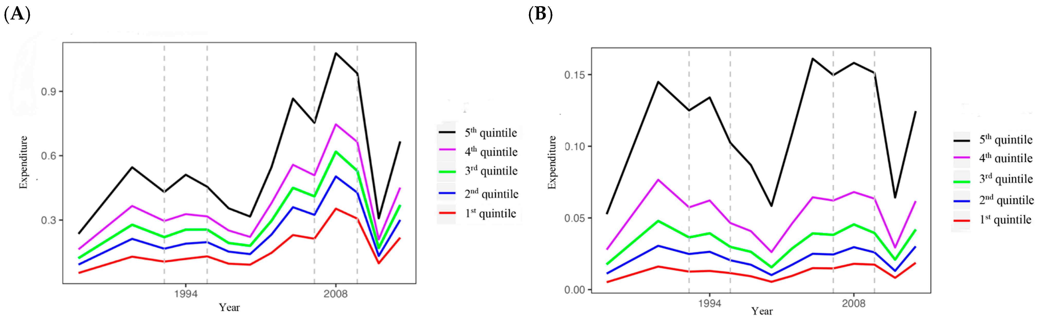
The elasticities of consumption concerning variations in income were shown for each household type and each category of goods. A decrease in income resulted in food consumption elasticities that approached zero or were more inelastic than the elasticities of other goods for each household type. This indicated that the coefficients increased as income was compromised, consumer perception changed, and food purchase was prioritized. Consequently, for each household category, the expenditure on non-durable and semi-durable goods, such as food and clothing, was higher than that allocated to purchasing any other good. Despite this trend, notable differences were observed in the elasticities of non-durable and semi-durable goods during the two moments of crisis (Figure 1). For example, in the case of the coefficients in food (Figure 1A), in the 1994 crisis, those who suffered the most remarkable changes in their food consumption patterns were households in the highest quintiles. Households in deciles 1, 2, and 3 hardly suffered any change at all. Conversely, in the 2008 crisis, the coefficients exhibited increases greater than one, signifying those fluctuations in consumption exhibited more excellent elasticity for all households, with the most pronounced increases observed among the least affluent quintiles.

In the context of clothing consumption patterns, Figure 1B reveals a parallel behavior in the coefficients to that observed in food consumption. However, the first and second quintile variations are negligible during the two crises. These quintiles distinguish these patterns from those observed in food consumption. The analysis indicates that these households exhibit low clothing consumption or a consumption pattern focused on essentials. The alterations in consumption patterns are more pronounced for the fourth and fifth quintiles, in which the elasticities become considerably more elastic. Consequently, their consumption is more susceptible to other factors that determine the demand curve, distinct from necessity.

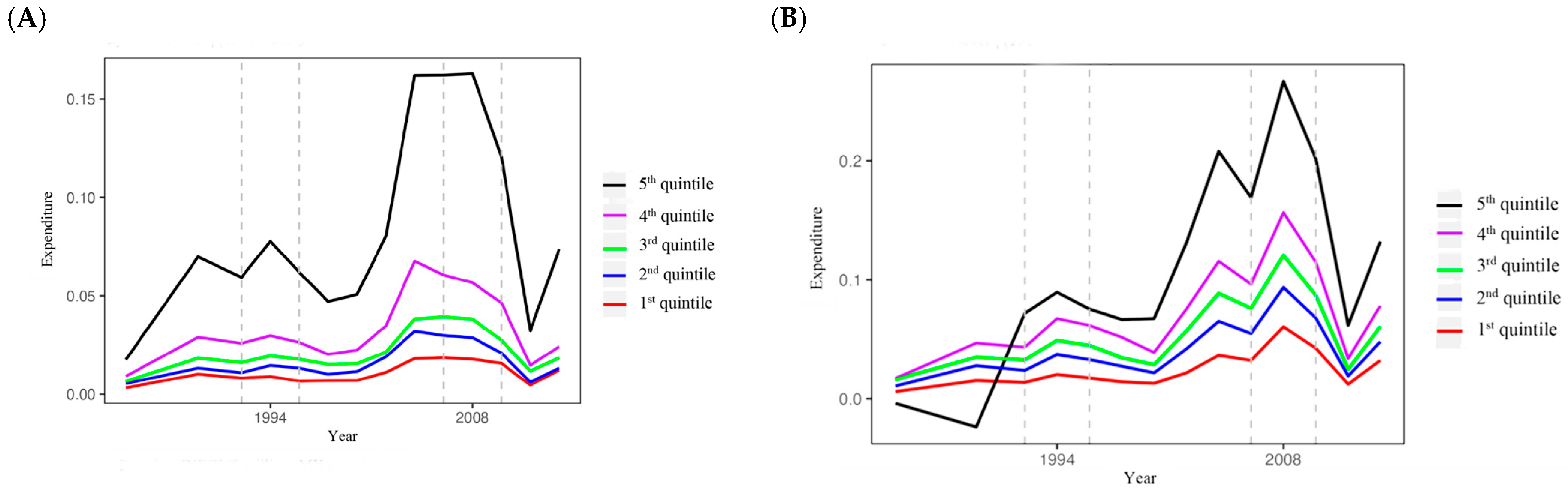
In contrast, health expenditures were the least significant for all income levels except for the fifth quintile. Figure 2A demonstrates that spending on this service, which could be categorized as a durable good, remained consistent for low-income households during both regular times and the crisis. However, the perception of this expenditure significantly changed during the 2008 crisis for Mexican households in the fifth quintile. This shift was due to the possibility of job loss or reduced income.

As illustrated in Figure 2A, expenditure on housing has experienced the most significant real-term increase across all income brackets. Indeed, since the mid-1990s, the share of the family budget allocated to housing has surpassed that of clothing—Mexican households in the third to fifth quintiles previously allocated more funds to clothing and health than housing. In Mexico, the budgetary allocation of families was predominantly directed towards housing payments, superseding expenditure on transport, education, leisure, and health. This phenomenon was attributable to the escalating prices of these goods. In recent years, the value of housing has exhibited a growth trajectory that significantly surpasses that of other commodities, compelling households to allocate a more significant proportion of their budget to housing expenditures.

As shown in

Table 2. The coefficients categorized by asset type and household concerning the gender variable.

Year	Non-Durable Goods (1)	Non-Durable Goods (2)	Non-Durable Goods (3)	Non-Durable Goods (4)	Non-Durable Goods (5)	Semi-Durable Goods (1)	Semi-Durable Goods (2)	Semi-Durable Goods (3)	Semi-Durable Goods (4)	Semi-Durable Goods (5)
1994	−0.009	0.017	0.016	−0.011	−0.006	−0.0001	0.008	0.003	−0.004	0.007
1996	−0.004	−0.015	0.019 **	−0.008	−0.001	0.005	0.008	−0.006	0.029 **	0.006
1998	−0.028	0.024	0.011	−0.020 *	−0.016	−0.006	0.021	0.009	0.033 **	−0.014
2000	0.026	0.009	0.004	−0.024 **	−0.014	0.021	0.002	0.021	0.02	0.046 ***
2002	0.018	0.013	0.01	−0.005	0.001	0.018	0.02	0.01	0.031 **	0.009
2004	−0.003	0.011	−0.025 ***	−0.013	−0.003	0.029 **	0.022 **	0.024 *	0.033 **	0.017
2006	−0.018	−0.015	−0.017 *	−0.026 **	−0.015	0.016	0.033 *	0.025 **	0.023 **	0.036 ***
2008	0.12	−0.011	−0.001	−0.11 *	−0.01	0.006	0.032 **	0.026 **	0.021 **	0.031 ***
2010	−0.221 ***	−0.158 ***	−0.150 ***	−0.105 ***	−0.098 ***	−0.107 ***	−0.048 **	−0.061 **	−0.066 **	0.02
2012	−0.255 ***	−0.189 ***	−0.133 ***	−0.178 ***	−0.153 ***	−0.188 ***	−0.015	−0.053	−0.036	−0.036
Year	Durable Goods (1)	Durable Goods (2)	Durable Goods (3)	Durable Goods (4)	Durable Goods (5)	Services (1)	Services (2)	Services (3)	Services (4)	Services (5)
1994	0.043	−0.039	0.143	−0.02	0.038	0.035	0.037	0.03	0.018	0.005
1996	−0.022	−0.002	−0.012	0.035	−0.033	0.002	0.002	−0.002	0.039 **	0.039 **
1998	−0.022	0.043	0.002	0.061	0.047	0.04	0.024	−0.006	0.018	0.025
2000	−0.057	−0.064	−0.112	−0.07	−0.081	0.023	0.001	0.046 *	0.029	0.017
2002	−0.00002	0.082	0.031	0.044	0.031	0.037	−0.011	0.015	0.025	0.0002
2004	−0.015	−0.009	0.029	0.025	−0.61	0.027	0.009	0.022	0.021	0.026 ***
2006	−0.04	−0.07	−0.038	−0.072	−0.147 ***	−0.011	0.011	0.025	0.014	0.003
2008	−0.091 **	0.075 **	0.110 ***	0.033	0.01	−0.033	0.025	0.008	0.032 **	0.031 **
2010	0.129	0.339 ***	−0.333	0.066	0.042	−0.018	−0.142 ***	−0.125 ***	−0.130 ***	−0.098 **
2012	−0.304 *	−0.371 **	−0.179	−0.188 *	−0.189 **	0.077	0.132 *	0.063	−0.033	0.015

Note. The number in brackets denotes the quintile of the households. The asterisks indicate the level of significance of the coefficients. A high level of significance is indicated by three asterisks. A medium level of significance is indicated by two asterisks. A low level of significance is indicated by one asterisk.

, Mexican female-headed households generally allocate a smaller portion of their income to food during the early stages of economic development when financial resources are limited. However, the findings indicate that consumption patterns evolve across various socioeconomic levels over time. The non-significant coefficients suggest no notable shifts in consumption behaviors among female-headed households during the economic crisis of 1994. In contrast, during stable periods, the opposite seems accurate, as households with a female primary income earner allocate a larger share of their expenditures to clothing, footwear, and personal hygiene items than those led by men. They prioritize spending on these items over other categories, such as durable goods, education, or healthcare services.

As

Table 3. The coefficients categorized by asset type and household concerning the no school variable.

Year	Non-Durable Goods (1)	Non-Durable Goods (2)	Non-Durable Goods (3)	Non-Durable Goods (4)	Non-Durable Goods (5)	Semi-Durable Goods (1)	Semi-Durable Goods (2)	Semi-Durable Goods (3)	Semi-Durable Goods (4)	Semi-Durable Goods (5)
1994	0.123 ***	0.005	0.028	0.016	0.005	0.058 ***	0.043 ***	0.021	0.037 **	−0.004
1996	−0.504 ***	−0.051	−0.046	−0.080 ***	−0.034	−0.137 *	−0.104 ***	−0.043	0.001	−0.068 ***
1998	−0.777 ***	−0.223 *	−0.067	−0.003	−0.011	0.017	0.034	0.059	0.094 ***	−0.0002
2000	−0.288 ***	−0.188 ***	−0.714 ***	−0.066 **	−0.035	−0.133 ***	−0.037	−0.082 **	−0.072 **	−0.143 ***
2002	−0.303 ***	−0.268 ***	−0.719 ***	0.085 ***	−0.116 ***	−0.140 ***	−0.014	−0.071 ***	−0.086 ***	0.058
2004	−0.365 ***	−0.122 ***	−0.150 ***	0.066 ***	0.089 ***	0.04	−0.116 ***	−0.01	0.022	0.246 ***
2006	−0.043 ***	−0.238 ***	−0.234 ***	−0.195 ***	−0.455 ***	−0.120 ***	−0.106 ***	−0.143 ***	−0.131 ***	−0.036
2008	−0.286 ***	−0.211 ***	−0.108 ***	−0.161 ***	−0.124 ***	−0.089 ***	0.01	−0.075 ***	−0.016	−0.021
2010	−0.876 ***	−0.609 ***	−0.267 ***	−0.306 ***	−0.359 ***	−0.099	−0.158 ***	−0.221 ***	−0.193 ***	−0.256 ***
2012	−0.591 ***	−0.487 ***	−0.461 ***	−0.372 ***	−0.393 ***	−0.314 **	−0.157 *	−0.312 ***	−0.319 ***	−0.466 ***
Year	Durable Goods (1)	Durable Goods (2)	Durable Goods (3)	Durable Goods (4)	Durable Goods (5)	Services (1)	Services (2)	Services (3)	Services (4)	Services (5)
1994	0.012	−0.150 **	0.132	0.051	−0.100 *	−0.135 ***	0.02	−0.024	−0.037	0.002
1996	−1.678 ***	−0.475	−0.828 ***	−1.167 ***	−0.418 ***	0.085	−0.401 ***	−0.304 ***	−0.397 ***	−0.350 ***
1998	−1.678 ***	−1.003 ***	−0.634 ***	−0.616 ***	−0.357 ***	−0.564 **	−0.608 ***	−0.469 ***	−0.482 ***	−0.241 ***
2000	−0.797 ***	−0.438 ***	−0.555 ***	−0.762 ***	−1.329 ***	0.477 ***	−0.06	−0.110 ***	−0.533 ***	−0.629 ***
2002	−1.999 ***	−2.075 ***	−1.766 ***	−1.563 ***	−1.162 ***	0.053	−0.055	−0.163 ***	−0.352 ***	−0.419 ***
2004	−0.422 ***	−0.353 ***	−0.399 ***	−0.633 ***	0.543 ***	0.034	−0.446 ***	−0.322 ***	−0.462 ***	−0.645 ***
2006	−0.768 ***	−0.712 ***	−1.076 ***	−0.891 ***	−0.573 ***	0.448 ***	−0.295 ***	−0.411 ***	−0.463 ***	−0.625 ***
2008	−0.876 ***	−1.101 ***	−1.209 ***	−1.330 ***	−0.746 ***	0.431 ***	0.0833 **	−0.139 ***	−0.203 ***	−0.135 ***
2010	−3.760 ***	−2.560 ***	−1.828 ***	−1.627 ***	−1.176 ***	0.135	−0.360 ***	−0.526 ***	−0.512 ***	−0.546 ***
2012	−3.118 ***	−2.019 ***	−2.011 ***	−1.499 ***	−0.967 ***	0.402	−0.231	−0.572 ***	−0.494 ***	−0.528 ***

Note. The number in brackets denotes the quintile of the households. The asterisks indicate the level of significance of the coefficients. A high level of significance is indicated by three asterisks. A medium level of significance is indicated by two asterisks. A low level of significance is indicated by one asterisk.

shows, households with a basic level of education reported lower pre-crisis expenditures on each good than households with a higher education level. However, initial expenditure on durable goods is lower for uneducated Mexican households and greater for educated households, suggesting that middle-income families had a larger initial budget for purchasing cars, houses, furniture, and large appliances (durable goods). Furthermore, as indicated by the head of the household, Mexican households with a high school education or less experienced a more significant reduction in income dedicated to semi-durable goods and services. This trend was particularly evident during the 2008 crisis compared to the 1994 crisis for these households.

In contrast, households with a higher level of education showed greater initial expenditures on clothing and footwear, personal hygiene products, education, health, and transportation (

Table 4. The coefficients categorized by asset type and household concerning the school variable.

Year	Non-Durable Goods (1)	Non-Durable Goods (2)	Non-Durable Goods (3)	Non-Durable Goods (4)	Non-Durable Goods (5)	Semi-Durable Goods (1)	Semi-Durable Goods (2)	Semi-Durable Goods (3)	Semi-Durable Goods (4)	Semi-Durable Goods (5)
1994	0.320 ***	0.133 ***	0.238 ***	0.074 ***	0.074 ***	0.092 ***	0.091 ***	0.074 ***	0.018	−0.005
1996	−0.293	0.018	0.014	−0.024	−0.029	−0.066	−0.009	0.066 *	0.057 **	0.008
1998	−0.813	−0.208 *	0.005	0.036	−0.002	−0.004	−0.02	0.01	0.043	0.034 *
2000	0.054	0.075	0.106 *	−0.041 **	−0.047 ***	−0.060 *	0.032	0.008	0.011	0.019
2002	−0.182 ***	−0.041	0.063 ***	0.059 ***	−0.026 ***	−0.118 ***	0.039 *	0.014	0.01	0.083 ***
2004	−0.I39 ***	−0.041 **	−0.063 ***	0.023 **	−0.003	0.109 ***	−0.029 *	0.013	0.059 ***	0.125 ***
2006	−0.04	−0.053 ***	−0.031 **	−0.037 ***	−0.043 ***	−0.040 **	−0.028 *	−0.027 *	−0.009	0.028 ***
2008	−0.024	−0.070 ***	−0.056 ***	−0.069 ***	−0.064 ***	−0.040 **	0.023	0.011	−0.004	−0.007
2010	−0.534 ***	−0.328 ***	−0.179 ***	−0.120 ***	−0.190 ***	−0.017	−0.022	−0.087 ***	−0.087 ***	−0.160 ***
2012	−0.307 *	−0.038	−0.213 ***	−0.166 ***	−0.180 ***	−0.0002	0.034	−0.049	−0.053	−0.183 ***
Year	Durable Goods (1)	Durable Goods (2)	Durable Goods (3)	Durable Goods (4)	Durable Goods (5)	Services (1)	Services (2)	Services (3)	Services (4)	Services (5)
1994	0.464 ***	0.037	0.376 ***	0.298 ***	0.348 ***	0.139 ***	0.274 ***	0.289 ***	0.177 ***	0.175 ***
1996	−1.524 ***	−0.41	−0.841 ***	−0.893 ***	−0.363 ***	−0.271	−0.396 ***	−0.282 ***	−0.283 ***	−0.251 ***
1998	−1.523 ***	−1.298 ***	−1.007 ***	−0.699 ***	−0.540 ***	−0.527 *	−0.546 ***	−0.437 ***	−0.388 ***	−0.336 ***
2000	−0.338 ***	0.057	−0.109	−0.447 ***	−0.834 ***	−0.169 *	−0.174 ***	−0.267 ***	−0.315 ***	−0.390 ***
2002	−1.773 ***	−1.270 ***	−0.815 ***	−0.627 ***	−0.474 ***	−0.230 **	−0.355 ***	−0.186 ***	−0.174 ***	−0.238 ***
2004	−0.049	0.109	−0.281 ***	−0.202 ***	−0.021	−0.262 ***	−0.311 ***	−0.234 ***	−0.339 ***	−0.366 ***
2006	−0.251 ***	−0.288 ***	−0.197 ***	−0.176 ***	−0.293 ***	−0.164 ***	−0.128 ***	−0.188 ***	−0.208 ***	−0.243 ***
2008	−0.200 ***	−0.543 ***	−0.536 ***	−0.625 ***	−0.391 ***	0.107 **	0.027	−0.035	−0.062 ***	−0.062 ***
2010	−2.530 ***	−1.530 ***	−0.931 ***	−0.540 ***	−0.421 ***	−0.225	−0.285 ***	−0.407 ***	−0.232 ***	−0.238 ***
2012	−1.755 ***	−0.846 *	−0.857 ***	−0.657 ***	−0.421 ***	0.226	−0.222	−0.235 **	−0.215 **	−0.218 ***

Note. The number in brackets denotes the quintile of the households. The asterisks indicate the level of significance of the coefficients. A high level of significance is indicated by three asterisks. A medium level of significance is indicated by two asterisks. A low level of significance is indicated by one asterisk.

). The relationship between educational attainment and income is such that lower-income households spend a larger portion of their income on food.

As demonstrated in the preceding tables, the initial expenditure of Mexican households on durable goods, services, and semi-durables was negative, with a greater degree of negativity observed in the case of durable goods. This indicated that irrespective of income level, educational attainment, or gender of the head of household, families spent less on these goods. This observation was particularly pertinent in luxury goods, given their long useful lives, cost, and durability. Furthermore, the constants of non-durable goods were positive, indicating that Mexican households invariably commenced with a positive initial expenditure on food irrespective of income level.

Finally, the fact that the poorest households spend a significant part of their income on food consumption explains the higher coefficients for non-durable goods. At the same time, their budgetary constraints forced them to allocate their low income to other intermediate needs such as housing, clothing, and education. For their part, high-income households experienced a greater income effect on food consumption through increased quantity available and improved variety and origin. In addition, these households tend to have more resources to spend on various ‘high-end’ services such as travel, private education, high-quality medical care, and personalized financial services. Therefore, as observed for the second, third, and fifth quintiles, an increase in their income translated into a significant increase in their consumption of services. On the other hand, low-income households use part of their income to cover the most basic and necessary services, such as utilities, medical care, and transport, which are needed for life. Importantly, this behavior was not the best course of action, at least for the 1994 crisis.

4. Discussion

The crises being analyzed began in 1994 and 2008 when a sudden GDP reduction occurred. However, the adjustment in household consumption persisted until 1996 and 2010. In this respect, during the economic crisis of 1994, Mexican households generally reduced their food consumption. Although this effect was widespread, the decrease was more significant and prolonged in higher-income households. These Mexican households also exhibited a more pronounced and protracted decline in clothing, housing, and health expenditures, as evidenced by Figure 1A,B and Figure 2A,B. Conversely, for Mexican households in the first three quintiles, the coefficients for non-durable and semi-durable goods exhibited greater rigidity, indicating that spending on food, clothing, and personal hygiene items demonstrated less responsiveness to fluctuations in income. Conversely, spending on services exhibited a greater propensity to fluctuate in response to a decline in revenue.

In contrast, during the 2008 crisis, as illustrated in the previous figures, there was a substantial decline in the consumption of all goods, indicating that the 2008 crisis was more detrimental for all Mexican households. Despite the decline in consumption, spending on durable goods experienced a temporary decrease, with a recovery occurring two years later. Consequently, this outcome might signify an adjustment in consumption rather than a persistent trend. According to Engel’s theory, when a family budget is negatively impacted by income loss due to layoffs or when the possibility of layoff becomes a source of uncertainty, households tend to place a higher priority on food consumption over other durables goods. Concerning the salient variables, households headed by women exhibited an initial expenditure on food and durable goods that was lower than the income–expenditure effect observed at regular times during the 1994 crisis. Concurrently, this Mexican household profile demonstrated a higher initial expenditure on services and semi-durable goods. In contrast, during the 2010 crisis, these households initiated negative initial spending on all goods except luxury goods.

Regarding the level of education variable, Mexican households with upper-secondary qualifications exhibited higher food expenditures during both periods than those with lower qualifications. According to the initial expenditures on semi-durable goods, Mexican households with a low level of education allocated smaller budgets. In contrast, the rest allocated more initially, except for the years of the economic crisis, during which this consumption category contracted more than households with less education. These results are in line with those obtained by Fuentes and Rojas (2001), McKenzie and Mall (2001), Hernández-Tezoquipa et al. (2005) and Wang and Zhao (2023) in that consumption patterns change as income levels change. There is an Engel effect in households, where the level of consumption is reduced in the face of an increase in income. However, like McKenzie and Mall (2001), it was observed that in the face of an income shock, as in the 1994 crisis, the less educated sectors reduced their consumption. This situation is because these Mexican households depend on financial transfers from abroad rather than on current wages, mainly those from Mexican immigrants in the United States, who offered relief from falling purchasing power. This was not the case for the 2008 crisis, in which the contagion was widespread, and the response depended on the initial socioeconomic conditions.

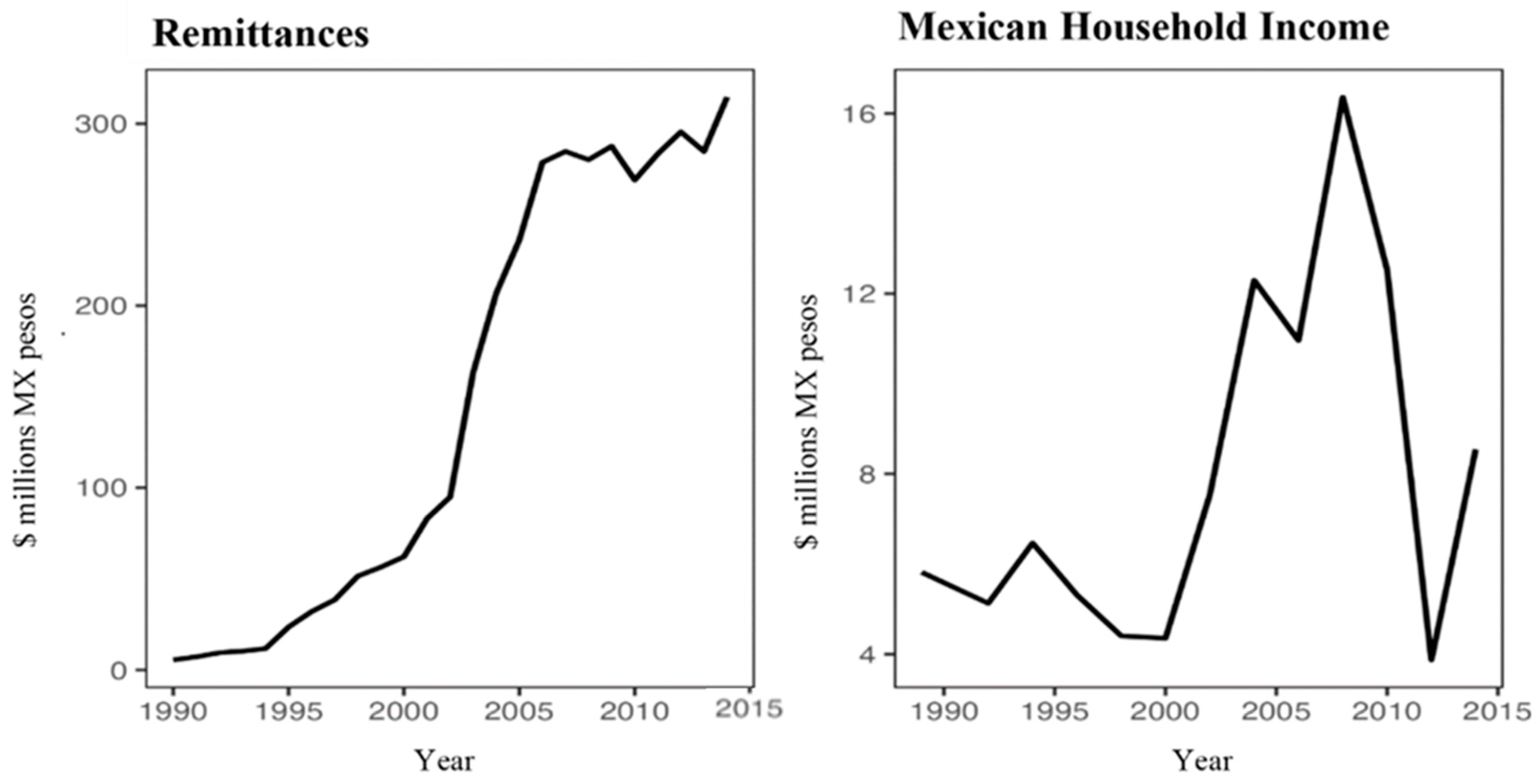
According to the Banco de México (2010) and the Mexican National Institute of Statistics and Geography (INEGI 1994–2012), remittances received by Mexicans exhibited consistent growth before the 2008 economic crisis, during which a significant decline occurred, as illustrated in Figure 3. After five years, this decline was reversed, and growth accelerated. The reports also showed a correlation between higher levels of remittance income and higher income. This finding suggests that, as poorer and less educated households lost access to remittances, their spending behavior followed the expected patterns outlined by the theoretical framework during the crisis. Conversely, higher remittance income led to unexpected consumption patterns among the poorest and higher-income households. The crisis of 2008 served as an indirect confirmation of these results.

The results of this study align with the conclusions of López-Romero (2021), Moreno-Brid and Ros (2009), and Luna and Nolasco (2004), who asserted that the economic cycles of the United States and Mexico have exhibited a high degree of codependency over several decades. This codependency has seriously affected the Mexican economy, which is significantly disadvantaged. While the United States has historically served as a market for Mexican goods, the intricacies of culture, environment, monetary policy, and fiscal policy have imposed considerable challenges, further exacerbating the economic disparities between the two nations. A notable example is the 2008 crisis, which originated in the United States. In the aftermath of this crisis, there were limited domestic policy mechanisms available to stimulate the economy, and there was a conspicuous absence of financial assistance or investments from Mexico, the United States’ primary commercial and cultural partner, to mitigate the adverse effects of the crisis (Economic Commission for Latin America and the Caribbean (ECLAC) 2009; Villareal 2010). This stands in contrast to the 1994 crisis, which, although originating internally, was addressed through external measures.

In their research, Feenstra and Taylor (2008) confirmed that the signing of the North American Free Trade Agreement (NAFTA), now known as the United States–Mexico–Canada Agreement, has contributed significantly to the interconnection of the economic cycles of the economies that comprise North America. In their study, the authors found that from 1994 to 2000, the maquiladoras’ productivity on the United States border experienced a high compound growth rate of 4.1% per year. The authors identified several factors contributing to this growth, including the effects on investment attracted by the signing of the trade agreement, the transfer of technology, and the integration of semi-skilled workers on both sides of the northern border. Furthermore, Arévalo and Herreros (2015) found that the impact of the 2008 crisis was more significant in the region’s north than in the south due to the commercial connection. The authors documented substantial job losses in the northern region, while the southern region experienced modest growth. From their vantage point, this phenomenon exacerbated regional vulnerability and inequality within the country.

The extant literature, including the present study, has identified the importance of promoting targeted social support programs to generate positive income in the family budget. In this respect, various social programs have been implemented that have positively affected aggregate demand in times of crisis and have avoided reducing the quantity and quality of food consumption. However, as Kremer and Holla (2009) emphasize, sustaining the focus on such programs is imperative, ensuring that expenditures on education and health services, which tend to be less conspicuous, suffer during economic adversity. Doing so can mitigate the impediments to economic growth and societal welfare.

The ENIGH data from 1994 to 2021 demonstrated that households of all types adjusted their spending during economic crises. However, the spending on non-durable goods exhibited lower elasticity, indicating that consumers were less willing to reduce this essential spending when their income decreased. The lower adjustment in the consumption of these goods was due to increased prioritization in the consumption pyramid, given their lower prices than other goods. The constant associated with each good indicated that households tended to have negative initial spending on durable goods, services, and semi-durable goods during crises. However, this negative initial expenditure was more pronounced in the case of durable goods.

The findings concerning the variables of interest—namely, income, gender, and education within the household—were unambiguous: initial expenditures on durable goods (considered luxury goods) were negative. Regarding gender, female-headed households commenced with a lower initial expenditure on food and durable goods. However, this household profile exhibited higher spending on services and semi-durable goods. Notably, despite the economic downturn in 2008, there was an increase in the consumption of clothing and luxury goods, despite households initially incurring a negative expenditure on all goods. Furthermore, the impact of the 1994 crisis on consumption levels was less significant for less educated households than the 2008 crisis. This would facilitate the identification of the most vulnerable households, thereby enabling targeting programs to the most at-risk populations and averting the exacerbation of poverty rates during periods of economic downturn. The present study underscores the necessity of an ongoing analysis of the long-term implications of synchronized economic cycles between the U.S. and Mexico. It also highlights the pressing need to enhance our understanding of these two nations’ cultural, social, and economic interrelationships in order to ensure development convergence.

5. Conclusions

Economic crises inevitably impact Mexican household incomes, regardless of their origin. However, external factors can either amplify or mitigate their effects. The 1994 crisis, for example, disproportionately affected higher-income households. Despite the economic disruption, these households demonstrated greater resilience, partly due to substantial remittance inflows from the United States, driven by its strong economic growth. In contrast, the 2008 crisis, originating in the United States, impacted Mexico differently. It led to a decline in the volume and value of remittances received by the poorest households and caused a slowdown in Mexican exports. These outcomes reignited debates on the vulnerabilities of Mexico’s economic dependence on the United States and the lack of adequate policies to buffer external shocks. Recognizing household vulnerabilities based on social and educational factors is crucial when designing poverty alleviation programs. Our study incorporated gender and education variables to identify the most at-risk populations, ensuring targeted assistance to prevent worsening poverty during economic downturns. Additionally, the findings emphasize the need for continued research on the long-term effects of synchronized economic cycles between Mexico and the U.S. and the broader implications of their social, cultural, and economic interdependence.

In addition, it would be pertinent to incorporate geographical variables in future studies, encompassing both regional and rural–urban differences. Extant evidence indicates considerable variations in the intensity and duration of shocks according to these conditions. Furthermore, it would be advantageous to concentrate the analysis exclusively on durable goods, given that they exhibit a high degree of sensitivity during periods of economic downturn and serve as a critical indicator of households’ financial well-being. This would facilitate a more nuanced understanding of the mechanisms governing consumption adjustment and enable the formulation of targeted public policies that would foster the economic resilience of the most vulnerable sectors.