Susceptibility of a Multivariate Approach to the Measurement of Neighborhood-Level Socioeconomic Status in Neighborhoods and Health Research: Descriptive Findings with Analytical Reasoning

Oka, Masayoshi

doi:10.3390/socsci13120693

Open AccessArticle

Susceptibility of a Multivariate Approach to the Measurement of Neighborhood-Level Socioeconomic Status in Neighborhoods and Health Research: Descriptive Findings with Analytical Reasoning

by

Masayoshi Oka

Department of Management, Faculty of Management, Josai University, Sakado 350-0295, Japan

Soc. Sci. 2024, 13(12), 693; https://doi.org/10.3390/socsci13120693

Submission received: 4 November 2024 / Revised: 12 December 2024 / Accepted: 16 December 2024 / Published: 19 December 2024

Download

Browse Figures

Versions Notes

Abstract

:

A fairly large number of area-based indices have been developed in the United States (US) and other countries to examine the contextual effect of neighborhood-level socioeconomic status (SES) on health. However, two conceptual and methodological review articles raised several concerns about a multivariate approach to the measurement of neighborhood-level SES. To untangle some of the conceptual and methodological concerns raised in those review articles, the purpose of this study was to illuminate a couple of common oversights masked by the lack of analytical transparency in neighborhoods and health research. Using the State of California and its seven Metropolitan Statistical Areas as the study areas, census-tract-level population estimates from the 2000 Census as well as the 2005–2009, 2010–2014, and 2015–2019 American Community Survey were obtained from the United States Census Bureau’s website for conducting a sequence of data analyses. The results of this study suggest that a multivariate approach to the measurement of neighborhood-level SES may be susceptible to the spatial size and spatial configuration of geographic areas and/or the population size and population structure of geographic areas. For these reasons, a few underlying sources of measurement uncertainty, which may undermine the generalizability of existing area-based indices and their measurement validity, are discussed in a general sense so as to be relevant for examining the contextual effect of neighborhood-level SES on health in the US and other countries.

Keywords:

neighborhood advantage; neighborhood disadvantage; neighborhood deprivation; composite population; areal median filtering; spatial approaches

1. Introduction

Research inquiries into the role of place of residence in health has a long history, where its origins can be traced back to the pioneering work by an English physician John Snow in the 1840s and 1850s (Vinten-Johansen et al. 2003), although the seminal works by a German physician Leonhard L. Finke in the 1790s (Barrett 1993, 2000) and by an American physician Daniel Drake in the 1850s (Barrett 1996) have also been credited for their important contributions in medical geography. Fueled by the availability of geospatial data and the advancement of geographic information systems since the turn of the 21st century, the past two decades have witnessed an explosive growth of interest in neighborhoods and health research (Arcaya et al. 2016), not only focusing on infectious or vector-borne diseases, but also on various health behaviors and health conditions. While the study of neighborhoods and health has become one of the mainstream topics in public health (Diez Roux 2016), this line of research revolves around the interface between social sciences and public health (Entwisle 2007; Matthews and Parker 2013) for which to understand how the physical and/or social characteristics of neighborhoods shape the health of individuals residing in them (Duncan and Kawachi 2018; Kawachi and Berkman 2003).

Among a variety of neighborhood characteristics considered in the United States (US) and elsewhere, several review articles collectively suggest that individuals living in neighborhoods of lower socioeconomic status (SES) tend to experience increased risks of poor health, such as unhealthy diet, physical inactivity, and obesity (Black and Macinko 2008; Booth et al. 2005), depression or depressive symptoms (Kim 2008; Mair et al. 2008), coronary heart disease (Chaix 2009), all-cause mortality (Meijer et al. 2012), adverse perinatal outcomes (Vos et al. 2014), preterm birth and low birthweight (Ncube et al. 2016), cognitive impairment among older adults (Besser et al. 2017), cumulative burden of chronic stress and life events (Ribeiro et al. 2018), frailty (Fritz et al. 2020), and lower cancer survival (Namin et al. 2021), relative to individuals living in neighborhoods of higher SES. In these reviewed studies conducted in the US, census tracts have been commonly used to denote neighborhoods and multilevel regression models (e.g., Gelman and Hill 2007; Hox et al. 2017; Raudenbush and Bryk 2002; Snijders and Bosker 2012) have been used to examine the contextual effect of neighborhood-level SES on an individual-level outcome of interest after adjusting for individual-level socioeconomic characteristics (e.g., age, gender, race/ethnicity, marital status, educational attainment, income level, and occupational status). Note that the terms “(dis)advantage”, “deprivation”, “socioeconomic (dis)advantage”, “socioeconomic deprivation”, and “socioeconomic position” have been used synonymously with “SES” to refer to the same dimension of neighborhood socioeconomic characteristics in the literature.

For the measurement of neighborhood-level SES, an area-based index has been used to combine multiple census-tract-level SES indicators (i.e., population estimates appertaining to income, poverty, employment, education, occupation, social welfare, and living conditions) into a composite measure (i.e., a unidimensional measure). While a fair number of area-based indices has been developed by different authors in the US (e.g., Diez Roux et al. 2001; Kind et al. 2014; Krieger et al. 2002; Messer et al. 2006; Morenoff 2003; Sampson et al. 1997; Singh 2003; Winkleby and Cubbin 2003; Yost et al. 2001), a sum of z-scores, factor analysis (FA), or principal component analysis (PCA) has been used as the computational method for deriving a composite measure of neighborhood-level SES. In other words, a composite measure of neighborhood-level SES refers to an unweighted summary score or a weighted summary score (i.e., a first factor score or a first component score) derived from one of these multivariate techniques. Using small enumeration units (i.e., administrative or statistical units equivalent to the US census tracts), similar area-based indices have also been developed in other countries, including, but not limited to, Canada (e.g., Pampalon et al. 2009; Pampalon and Raymond 2000), Denmark (e.g., Meijer et al. 2013; Pedersen and Vedsted 2014), France (e.g., Havard et al. 2008; Pornet et al. 2012), New Zealand (Salmond et al. 1998; Salmond and Crampton 2012), Spain (e.g., Benach and Yasui 1999; Domínguez-Berjón et al. 2008), Sweden (e.g., Bajekal et al. 1996; Sariaslan et al. 2013), and the United Kingdom (e.g., Carstairs and Morris 1989; Townsend et al. 1988).

While a handful of composite measures have been shown to yield similar results in the US (Krieger et al. 2002; Krieger et al. 2003a, 2003b, 2003c; Yu et al. 2014), two conceptual and methodological reviews of existing area-based indices (Allik et al. 2020; Sorice et al. 2022) raised several concerns about a conventional multivariate approach to the measurement of neighborhood-level SES. Among them, the development process of existing area-based indices has largely overlooked the importance of spatial thinking (Goodchild et al. 2000; Goodchild and Janelle 2010; Logan et al. 2010; Logan 2012) in quantifying population compositions and their distributional patterns in geographic space. In other words, composite measures derived from existing area-based indices have been aspatial in nature, which fails to account for spatial relationships between census tracts (or its equivalent administrative or statistical units). Hereafter, the term “aspatial” (not “non-spatial”) refers to the insensitivity of analytical results to a spatial arrangement of small enumeration units. More importantly, an exchangeability between two sets of mutually opposite census-tract-level SES indicators has not been examined in the development process of existing area-based indices and their application in neighborhoods and health research. This is of particular concern because a set of census-tract-level high-SES indicators and another set of their respective low-SES counterparts incorporated into an area-based index has been presumed to produce two separate composite measures that are inverses of each other. From a sensitivity analysis point of view (Saltelli 2002), however, such a general notion may not hold true, primarily due to relative differences in the shape of frequency distributions. Therefore, existing area-based indices may not adequately capture a change from highest to lowest SES neighborhoods or vice versa, thereby undermining their measurement validity and their usefulness in neighborhoods and health research; see Bartlett and Frost (2008), Bannigan and Watson (2009), and/or Heale and Twycross (2015) for the importance of measurement validity in all fields of study.

To untangle some of the conceptual and methodological concerns raised by Allik et al. (2020) and Sorice et al. (2022), the purpose of this study was to illuminate a couple of common oversights masked by the lack of analytical transparency on the exploratory data analysis of existing area-based indices. In order to capture residents’ daily experiences in residential space (Perchoux et al. 2013), a sequence of data analyses was carried out by implementing two spatial approaches (Oka and Wong 2016; Wong 1998) to provide a more realistic representation of neighborhoods. However, since Sorice et al. (2022) identified twenty-four different area-based indices developed in the US and used in cancer research (exclusive of those used in other fields of study), an examination of shortcomings for each area-based index was not possible. Therefore, a few underlying sources of measurement uncertainty overlooked by Allik et al. (2020) and Sorice et al. (2022), which may undermine the generalizability of existing area-based indices and their measurement validity, are discussed in a general sense so as to be applicable to a large number of area-based indices developed in the US and other countries.

2. Study Design

This study was built upon the findings and suggestions of Oka (2015, 2023) for choosing the reference measures of neighborhood-level SES. While less recognized (or underappreciated) in neighborhoods and health research, he showed that census-tract-level median household income (MHI) and median family income (MFI) were very strongly and positively correlated with each another and were also strongly or very strongly correlated, either positively or negatively, with five aspatial composite measures of neighborhood-level SES derived from five different area-based indices (Diez Roux et al. 2001; Krieger et al. 2002; Messer et al. 2006; Singh 2003; Winkleby and Cubbin 2003) in various geographic areas of the conterminous US (Oka 2015, 2023). With reference to the interchangeability of MHI with one or more aspatial composite measures of neighborhood-level SES (Krieger et al. 2002, 2003b, 2003c; Mode et al. 2016; Oka 2021) demonstrated in various geographic areas of the US, Oka (2015, 2023) suggested that either MHI or MFI may be used to capture a change of neighborhood-level SES from the lowest to the highest and, by multiplying or dividing MHI and MFI by −1 (denoted as MHI* and MFI*, respectively), either of their reversed form may be used to capture a change of neighborhood-level SES from the highest to the lowest. For these reasons, MHI and MFI as well as MHI* and MFI* were used to ensure the directionality and dimensionality of neighborhood-level SES in this study.

Since Oka (2023) examined a wide array of geographic ranges (i.e., spatial variations in the spatial size and spatial configuration of geographic areas as well as the population size and population structure of geographic areas) and their demographic changes at four different time periods (i.e., temporal variations in the population size and population structure of geographic areas), the State of California and its seven MSAs were considered as the study areas and population estimates from the 2000 Census as well as the 2005–2009, 2010–2014, and 2015–2019 American Community Survey (ACS) were used for a sequence of data analyses. As a brief explanation of these data, the ACS is an ongoing, nationwide survey conducted annually by the United States Census Bureau that provides vital information on demographic, social, economic, and housing characteristics of the US population (United States Census Bureau 2023). It replaced the long form of decennial censuses after the 2000 Census by collecting long-form-equivalent questionnaires every year, rather than once every ten years. While the ACS data are comparable with the 2000 Census data, only the basic population characteristics (e.g., age, gender, race or ethnicity, household size, and home ownership status) are comparable with the 2010 or 2020 Census data (United States Census Bureau 2024). Therefore, this study was built upon the study design contemplated by Oka (2023) to capitalize on the reliable aspatial measures of neighborhood-level SES (i.e., MHI and MFI as well as MHI* and MFI*) and to avoid the measurement uncertainty inherent in existing area-based indices pointed out by Allik et al. (2020) and Sorice et al. (2022).

Unlike any aspatial composite measures of neighborhood-level SES, the use of MHI or MFI, or alternatively MHI* or MFI*, provides a simple, yet consistent way of understanding a change of neighborhood-level SES from the lowest to the highest, or alternatively the highest to the lowest, in a consistent manner (Oka 2015, 2023). More importantly, such conceptualizations come with a set of practical benefits: little time for preparation; less effort on exploratory data analysis and map visualization; very few missing estimates within a given study area; reasonable standard of precision with a margin of error at the 90% confidence level across different geographic areas; consistent interpretation and straightforward comparison of research findings for research synthesis; and effective dissemination and mutual understanding of scientific evidence or scientific knowledge across academic disciplines and professional fields (Oka 2023). Given the widely accepted use of MHI and MFI in social sciences as two important indicators of economic well-being (primarily at the census tract, county, and state levels), Oka’s conceptualizations (Oka 2015, 2023) are justifiable in most geographic areas of the conterminous US (except for the State of Alaska and Hawaii, which are often regarded as geographic outliers).

3. Materials and Methods

3.1. Data

Together with MHI and MFI, population estimates appertaining to poverty status (above poverty and below poverty), employment status (employed and unemployed), educational attainment (Bachelor’s degree or higher and no high school diploma), social welfare status (no public assistance income and with public assistance income), and annual income (household income greater than or equal to USD 100,000 and household income less than USD 25,000) at the census tract level were obtained from the United States Census Bureau’s website (https://data.census.gov/table; accessed on 5 June 2024). These were selected from a list of common census-tract-level SES indicators incorporated into existing area-based indices (Sorice et al. 2022) and used as single measures of neighborhood socioeconomic characteristics (van Vuuren et al. 2014). Note that the United States Census Bureau classifies annual household income into sixteen categories. Therefore, the four highest and four lowest categories (out of these sixteen categories) were used to distinguish high- and low-income groups. These two groups were intended to be conservative and generalizable to the State of California and its seven MSAs. Hereafter, the term “high socioeconomic groups” refers to populations who were above poverty, were employed, held a Bachelor’s degree or higher, received no public assistance income, and earned an annual household income of greater than or equal to USD 100,000, and the term “low socioeconomic groups” refers to populations who were below poverty, were unemployed, had no high school diploma, were supported with public assistance income, and earned an annual household income of less than USD 25,000.

For implementing the concepts of composite population (Wong 1998) and areal median filtering (Oka and Wong 2016) in the next section, the 2000 and 2010 cartographic boundary shapefiles of census tracts were obtained from the United States Census Bureau’s website (https://www.census.gov/cgi-bin/geo/shapefiles/index.php; accessed on 5 June 2024). Note that census tract boundaries are updated once per decade to reflect population change (i.e., split or merged to account for population growth or decline). Since cartographic boundaries include lakes and ponds and extend into rivers and streams, such bodies of water were removed from these two cartographic boundary shapefiles using the erase tool in ArcGIS Desktop (ESRI Inc., Redlands, CA, USA). The shapefile of bodies of water was obtained from the Data & Maps Collection for ArcGIS on DVD, and all shapefiles were projected using the NAD 1983, State Plane Coordinate System. Then, the total land area (in square kilometers) was recalculated to better represent the actual land surface area of the study area. By removing bodies of water, therefore, the modified 2000 and 2010 cartographic boundary shapefiles provide a more realistic portrayal of the adjacency or contiguity of census tracts.

Based on these data, a brief description of the study areas is summarized in Table 1 where the seven most populous MSAs in the State of California are arranged by the number of total populations in descending order. Note that MSAs are delineated by the Office of Management and Budget (OMB) to reflect economic ties (defined by commuting patterns) and thus comprise one or more counties depending on the local economic activities. Also, the number of total populations are a summation of census-tract-level population estimates and may be susceptible to sampling and non-sampling errors, in spite of the United States Census Bureau’s efforts (United States Census Bureau 2022) to reduce such errors. For a detailed explanation on the nature and causes of uncertainty in population estimates, see a handbook published by the United States Census Bureau (2020).

3.2. Spatial Measures

A scoping review of activity space research (Perchoux et al. 2013) highlighted the need of taking into account for residents’ routine activities (e.g., household-, recreational-, social-, and travel-related activities) in a definition of neighborhoods; otherwise, an inadequate or ineffective representation of neighborhoods in epidemiologic research would lead to an unrealistic portrayal of residents’ exposure to their residential environment. For example, three studies (Basta et al. 2010; Jones and Pebley 2014; Zenk et al. 2011) conducted in different geographic areas of the US collectively showed that spatial patterns of residents’ routine activities extended from a census tract of residence into its surrounding census tracts. Therefore, the conventional use of census tracts in the US (or similar enumeration units in other countries) as a proxy for neighborhoods may be reasonable for residents living at or near the center of a census tract, but not for those living along or close to the border or edge of a census tract.

The conceptual and methodological limitations outlined by Perchoux et al. (2013) closely reflect the concerns raised by Allik et al. (2020) and Sorice et al. (2022) about the aspatial nature of composite measures of neighborhood-level SES. One way to address such limitations or concerns, the concept of composite population (Wong 1998) provides a more realistic portrayal of residents’ routine activities in their census tract of residence. In short, Wong (1998) introduced the

c_{i j} (.)

function to remove census tract boundaries as the absolute barriers for residents’ routine activities in geographic space by adopting the basic concepts of spatial association (Anselin 1995; Getis and Ord 1992) used in modeling spatial autocorrelation. Let census tract

i

be the reference census tract, the

c_{i j} (.)

function is a spatial binary matrix where

c_{i j} = 1

indicates census tracts

i

and

j

share a common boundary and

c_{i j} = N A

(not applicable) otherwise. Unlike the spatial weighting schemes (Bivand and Wong 2018; Getis 2009) implemented in spatial analysis, the

c_{i j} (.)

function includes the referent census tract and thus

c_{i i} = 1

(Wong 1998).

By implementing the

c_{i j} (.)

function into a census tract boundary shapefile, for example, the composite population counts of group G and total population (

{c g}_{i}

and

{c t}_{i}

, respectively) are computed as

{c g}_{i} = \sum c_{i j} g_{j}

(1)

and

{c t}_{i} = \sum c_{i j} t_{j}

(2)

where

g_{j}

is the population count of group G in census tract

j

and

t_{j}

is the population count of total population in census tract

j

. Therefore,

{c g}_{i}

is the population count of groups G in census tract

i

plus the population count of group G in one or more adjacent census tracts

j

and

{c t}_{i}

is the population count of total population in census tract

i

plus the population count of total population in one or more adjacent census tracts

j

. As a simplest application of the concept of composite population (Wong 1998), the composite proportion of group G (

{c p}_{i}

) is computed as

{c p}_{i} = {c g}_{i} / {c t}_{i}

(i.e., a spatial measure of the proportion of group G in census tract

i

).

Since the concept of composite population (Wong 1998) was designed to handle discrete data, the concept of areal median filtering (Oka and Wong 2016) was later introduced for handling interval or ratio data (e.g., median household income or population density). Capitalizing on the

c_{i j} (.)

function developed by Wong (1998), the areal median filtering (

{s m}_{i}

) is computed as

{s m}_{i} = m e d i a n \{c_{i j} q_{j}\}

(3)

where

q_{i}

is the value of interval or ratio data in census tract

j

. Put differently,

{s m}_{i}

is the spatial median of interval or ratio values in census tract

i

and its one or more adjacent census tracts

j

. Note that Oka and Wong (2016) recommended the use of median, instead of the mean (or the average), for quantifying the central tendency of neighborhood characteristics because a spatial mean (or average) would be affected by extreme values. Therefore, the concept of areal median filtering is a more robust approach than its alternative areal mean (or average) filtering (Oka and Wong 2016).

In this study,

{s m}_{i}

in Equation (3) was used to compute spatial measures of MHI and MFI (denoted as sMHI and sMFI, respectively) as well as MHI* and MFI* (denoted as sMHI* and sMFI*, respectively) and

{c p}_{i}

was used to compute spatial measures of high- and low-SES indicators. For the latter computation process,

{c g}_{i}

refers to the composite population count of five high and low socioeconomic groups described above, and

{c t}_{i}

the composite population count of population for whom poverty status was determined (i.e., the universe of above poverty and below poverty), civilian population 16 years and over in labor force (i.e., the universe of employed and unemployed), population 25 years and over (i.e., the universe of Bachelor’s degree or higher and no high school diploma), and households (i.e., the universe of no public assistance income and with public assistance income as well as of income greater than or equal to USD 100,000 and income less than USD 25,000) to properly reflect the universe of each socioeconomic group. Hereafter, the term “spatial high-SES indicators” refers to a composite proportion of residents who were above poverty (AP), were employed (EMP), held a Bachelor’s degree or higher (≥BD), received no public assistance income (NoPAI), and earned an annual household income of greater than or equal to USD 100,000 (≥$100K), and the term “spatial low-SES indicators” refers to a composite proportion of residents who were below poverty (BP), were unemployed (UNE), had no high school diploma (NoHSD), were supported with public assistance income (WithPAI), and earned an annual household income of less than USD 25,000 (<$25K).

As a technical note, census tracts immediately outside the state boundary of California were used to create an artificial buffer zone to avoid the boundary value problem (Griffith 1983) in this study. In other words, census tracts along the border of Arizona, Nevada, and Oregon that share a common boundary with census tracts in California (after removing bodies of water from the shapefiles as described above) were included in the computation of spatial medians (i.e.,

{s m}_{i}

) and composite population counts (i.e.,

{c g}_{i}

and

{c t}_{i}

) for the entire State of California. Widely regarded as one of the most common sources of computational bias in spatial analysis, the boundary value problem (Griffith 1983) arises from an inadequate examination of spatial relationships between enumeration units particularly along the border or edge of a study area. For handling such a computational bias in this study, using census tracts surrounding each of the study areas as an artificial buffer zone is justifiable because the

c_{i j} (.)

function introduced by Wong (1998) corresponds to the first-order adjacency of census tracts. Upon completing the computation processes, however, spatial measures within each of the study areas (i.e., omitting those in the artificial buffer zones) were only considered for further data analyses.

3.3. Data Analysis

A principal component analysis (PCA) was applied to five spatial high-SES indicators and five spatial low-SES indicators for deriving spatial composite measures of HIGH-SES and LOW-SES (labeled with uppercase letters), respectively, in each of the study areas at four different time periods. Since the socioeconomic makeup of a study area has been used as a fount of information for comparing research findings in literature, scoping, and/or systematic reviews, the overall percentages of socioeconomic groups in the study areas together with the component loadings of five spatial high-SES indicators and their respective low-SES counterparts are shown in Table 2, Table 3, Table 4, Table 5, Table 6, Table 7, Table 8 and Table 9.

For assessing an exchangeability between two sets of mutually opposite census-tract-level SES indicators (or lack thereof), which underlies at the heart of several conceptual and methodological concerns raised by Allik et al. (2020) and Sorice et al. (2022), a correlogram (Friendly 2002) was used to display the relationships between sixteen spatial measures described above. Since only subtle differences were observed at four different time periods, correlation matrices based on the 2015–2019 ACS data are shown in Figure 1, Figure 2, Figure 3, Figure 4, Figure 5, Figure 6, Figure 7 and Figure 8 and those based on the 2000 Census data as well as the 2005–2009 and 2010–2014 ACS data are provided in Supplementary Materials (Figures S1–S24). In these correlation matrices, Pearson’s correlation coefficients of pairwise relationships are laid out in the upper off-diagonal panels, an abbreviation for sixteen spatial measures with a density plot behind each abbreviation are listed in the diagonal panels, and scatterplots of pairwise relationships are presented in the lower off-diagonal panels. Building upon the findings and suggestions of Oka (2015, 2023), sMHI and sMFI were used as the reference measures for capturing a change of neighborhood-level SES from the lowest to the highest, whereas sMHI* and sMFI* were used as the reference measures for capturing a change of neighborhood-level SES from the highest to the lowest.

As a technical note, a sum of z-scores (or any other additive techniques) was not considered due to the lack of consensus on the optimal number and types of census-tract-level SES indicators incorporated into an area-based index (Allik et al. 2020; Sorice et al. 2022). As Folwell (1995) emphasized about three decades ago, additive techniques require a well-defined construct of neighborhood-level SES for their unweighted summary score (i.e., their composite measure) to be meaningful and generalizable. While a factor analysis (FA) may be considered as an alternative multivariate technique, skewed or highly skewed frequency distributions of input variables typically fail to satisfy the underlying assumption of multivariate normality, even if standard transformations (e.g., a square root, a logarithm with base 10, and a natural logarithm) were applied to reduce the skewness of input variables. Therefore, the use of PCA has been favored for capturing the multifactorial construct of SES in social sciences (e.g., Park et al. 2002); see Joliffe and Morgan (1992) and Schreiber (2021) for helpful explanations on the differences between FA and PCA. For these reasons, PCA was considered as the computational method of a hypothetical area-based index used in this study.

All computation and calculation processes were carried out in the R environment (R Core Team 2024). Besides the basic commands, a combination of functions in the spdep package (Bivand 2023) was used for implementing the

c_{i j} (.)

function (Wong 1998) into the modified 2000 and 2010 cartographic boundary shapefiles (after removing bodies of water); the princomp function in the stats package (a built-in or pre-installed package) was used for applying a sequence of PCAs to five spatial high-SES indicators and five spatial low-SES indicators; and the corrgram function in the corrgram package (Wright 2021) was used for displaying correlation matrices in Figure 1, Figure 2, Figure 3, Figure 4, Figure 5, Figure 6, Figure 7 and Figure 8 and in Supplementary Materials (Figures S1–S24).

4. Results

The State of California is located on the west coast of the US that stretches northward from the US–Mexico border along the Pacific Ocean for roughly 1450 km. As shown in Table 1, it encompasses a total land area of 402,887 km² and comprises 58 counties. With a steady population growth from about 33.9 million people to about 39.3 million people during the first two decades of the twenty-first century (i.e., a 1.16-fold increase), the number of census tracts also increased from 7049 in 2000 to 8037 in 2010 (i.e., a 0.88-fold increase). Within the State of California, Table 1 shows that its seven most populous MSAs also experienced a steady population growth (which ranges from a 1.07-fold increase in the Los Angeles–Long Beach–Anaheim MSA to a 1.40-fold increase in the Riverside–San Bernardino–Ontario MSA) and their number of census tracts also increased in a corresponding manner (which ranges from a 0.71-fold increase in the Riverside–San Bernardino–Ontario MSA to a 0.96-fold increase in the San Diego–Chula Vista–Carlsbad MSA). All in all, approximately 79.2 percent of Californias lived in these seven MSAs: about 34.9 percent in Los Angeles–Long Beach–Anaheim MSA, about 11.9 percent in San Francisco–Oakland–Berkeley MSA, about 10.9 percent in Riverside–San Bernardino–Ontario MSA, about 8.3 percent in San Diego–Chula Vista–Carlsbad MSA, about 5.7 percent in Sacramento–Roseville–Folsom MSA, about 5.0 percent in San Jose–Sunnyvale–Santa Clara MSA, and about 2.5 percent in Fresno MSA.

Table 1. Descriptions of the study areas.

	Total Land Area (km²) ^a	Census Tracts (#)		Counties(#)
	Total Land Area (km²) ^a	2000	2010	Counties(#)
State of California	402,887	7049	8037	58
Los Angeles–Long Beach–Anaheim MSA	12,572	2631	2924	2
San Francisco–Oakland–Berkeley MSA	6396	871	976	5
Riverside–San Bernardino–Ontario MSA	70,476	587	822	2
San Diego–Chula Vista–Carlsbad MSA	10,897	605	627	1
Sacramento–Roseville–Folsom MSA	13,191	403	484	4
San Jose–Sunnyvale–Santa Clara MSA	6930	349	383	2
Fresno MSA	15,447	158	199	1
	Total Population (#) ^b
	2000	2005–2009	2010–2014	2015–2019
State of California	33,871,648	36,308,527	38,061,951	39,278,430
Los Angeles–Long Beach–Anaheim MSA	12,365,627	12,762,126	13,055,565	13,244,547
San Francisco–Oakland–Berkeley MSA	4,123,740	4,218,534	4,466,251	4,701,332
Riverside–San Bernardino–Ontario MSA	3,254,821	4,022,939	4,345,485	4,560,470
San Diego–Chula Vista–Carlsbad MSA	2,813,833	2,987,543	3,183,143	3,316,073
Sacramento–Roseville–Folsom MSA	1,796,857	2,076,579	2,197,422	2,315,980
San Jose–Sunnyvale–Santa Clara MSA	1,735,819	1,784,130	1,898,457	1,987,846
Fresno MSA	799,407	890,750	948,844	984,521

^a Calculated using ArcGIS Desktop by the author. ^b Summation of census-tract-level population estimates. Abbreviation: MSA, Metropolitan Statistical Area.

The overall percentages of socioeconomic groups shown in Table 2a correspond to a representative description of Californians during the first two decades of the twenty-first century. Among the five mutually exclusive socioeconomic groups considered in this study, the overall percentages of populations who held a bachelor’s degree or higher increased by 7.31% (i.e., an increase from 26.62% to 33.93%) and those who had no high school diploma decreased by 6.51% (i.e., a decrease from 23.21% to 16.69%). In a similar manner, the overall percentages of populations who earned an annual household income of greater than or equal to USD 100,000 increased by 20.45% (i.e., an increase from 17.26% to 37.72%) and those who earned an annual household income of less than USD 25,000 decreased by 9.09% (i.e., a decrease from 25.49% to 16.40%). Otherwise, the overall percentages of other socioeconomic groups slightly increased or decreased during the four time periods, but their temporal changes were negligible.

Below the socioeconomic makeup of Californians at four different time periods (Table 2a), Table 2b shows the component loadings of five spatial high-SES indicators and their respective low-SES counterparts. Among them, composite proportions of residents who held a bachelor’s degree or higher (≥BD) and those who earned an annual household income of greater than or equal to USD 100,000 (≥$100K) were two spatial high-SES indicators that strongly and positively contributed to the spatial composite measures of HIGH-SES (i.e., the first principal component). On the other hand, composite proportions of residents who had no high school diploma (NoHSD) and those who earned an annual household income of less than USD 25,000 (<$25K) were two spatial low-SES indicators that strongly and positively contributed to the spatial composite measures of LOW-SES (i.e., the first principal component). While the values of component loadings during the four time periods fluctuated to a certain degree, their degrees of fluctuations were negligible.

Table 2. Overall percentages of high and low socioeconomic groups and component loadings of spatial high- and low-SES indicators in the State of California.

		Overall Percentages
a		2000	2005–2009	2010–2014	2015–2019
High Socioeconomic Groups
	Above Poverty	85.78%	86.79%	83.62%	86.64%
	Employed	92.99%	92.14%	89.01%	93.94%
	Bachelor’s Degree or Higher	26.62%	29.74%	31.00%	33.93%
	No Public Assistance Income	95.11%	96.75%	96.01%	96.77%
	Household Income ≥ USD 100,000	17.26%	27.41%	29.41%	37.72%
Low Socioeconomic Groups
	Below Poverty	14.22%	13.21%	16.38%	13.36%
	Unemployed	7.01%	7.86%	10.99%	6.06%
	No High School Diploma	23.21%	19.54%	18.51%	16.69%
	With Public Assistance Income	4.89%	3.25%	3.99%	3.23%
	Household Income < USD 25,000	25.49%	19.94%	20.45%	16.40%
		Component Loadings
b		2000	2005–2009	2010–2014	2015–2019
Spatial High-SES Indicators
	Above Poverty (AP)	0.33227	0.27138	0.31181	0.23316
	Employed (EMP)	0.14588	0.08975	0.12012	0.06990
	Bachelor’s Degree or Higher (≥BD)	0.74843	0.74009	0.72347	0.74147
	No Public Assistance Income (NoPAI)	0.15417	0.09063	0.09899	0.07344
	Household Income ≥ USD 100,000 (≥$100K)	0.53329	0.60196	0.59593	0.62095
Spatial Low-SES Indicators
	Below Poverty (BP)	0.40014	0.41652	0.48369	0.44621
	Unemployed (UNE)	0.15693	0.11056	0.14363	0.11129
	No High School Diploma (NoHSD)	0.71325	0.75329	0.70724	0.76245
	With Public Assistance Income (WithPAI)	0.16989	0.12364	0.14063	0.12426
	Household Income < USD 25,000 (<$25K)	0.52694	0.48120	0.47481	0.43789

Note: Five spatial high-SES indicators and their respective low-SES counterparts refer to the composite proportion of socioeconomic groups (see Equations (1) and (2)). Abbreviation: SES, Socioeconomic Status.

Partly reflecting the differences of population sizes (Table 1), the overall percentages of socioeconomic groups in seven MSAs (Table 3a, Table 4a, Table 5a, Table 6a, Table 7a, Table 8a and Table 9a) were somewhat different from those in the State of California (Table 2a) during the first two decades of the twenty-first century. In addition, the socioeconomic makeup of seven MSAs were also slightly different from one another (Table 3a, Table 4a, Table 5a, Table 6a, Table 7a, Table 8a and Table 9a). In accord with the temporal changes seen in the entire state of California (Table 2a), however, similar trends were also evident across seven MSAs (Table 3a, Table 4a, Table 5a, Table 6a, Table 7a, Table 8a and Table 9a): the overall percentages of populations who held a bachelor’s degree or higher, on average, increased by 7.50% (ranging between 3.63% and 11.64%) and those who had no high school diploma, on average, decreased by 5.96% (ranging between 4.75% and 8.49%); and the overall percentages of populations who earned an annual household income of greater than or equal to USD 100,000, on average, increased by 20.98% (ranging between 15.42% and 26.32%), and those who earned an annual household income of less than USD 25,000, on average, decreased by 8.19% (ranging between 3.77% and 12.11%). Otherwise, the overall percentages of other socioeconomic groups slightly increased or decreased during the four time periods, but their temporal changes were negligible in these seven MSAs.

Table 3. Overall percentages of high and low socioeconomic groups and component loadings of spatial high- and low-SES indicators in the Los Angeles–Long Beach–Anaheim Metropolitan Statistical Area (MSA).

		Overall Percentages
a		2000	2005–2009	2010–2014	2015–2019
High Socioeconomic Groups
	Above Poverty	83.84%	85.92%	82.92%	86.06%
	Employed	92.56%	92.64%	89.50%	94.27%
	Bachelor’s Degree or Higher	26.26%	30.00%	31.67%	34.47%
	No Public Assistance Income	94.48%	96.79%	96.15%	96.96%
	Household Income ≥ USD 100,000	17.03%	26.89%	28.92%	36.52%
Low Socioeconomic Groups
	Below Poverty	16.16%	14.08%	17.08%	13.94%
	Unemployed	7.44%	7.36%	10.50%	5.73%
	No High School Diploma	27.84%	22.73%	21.47%	19.35%
	With Public Assistance Income	5.52%	3.21%	3.85%	3.04%
	Household Income < USD 25,000	26.89%	20.76%	21.16%	17.26%
		Component Loadings
b		2000	2005–2009	2010–2014	2015–2019
Spatial High-SES Indicators
	Above Poverty (AP)	0.38517	0.30351	0.33079	0.24166
	Employed (EMP)	0.13618	0.07071	0.09129	0.04360
	Bachelor’s Degree or Higher (≥BD)	0.72895	0.72732	0.72756	0.76130
	No Public Assistance Income (NoPAI)	0.17881	0.09349	0.10087	0.07655
	Household Income ≥ USD 100,000 (≥$100K)	0.51938	0.60428	0.58542	0.59520
Spatial Low-SES Indicators
	Below Poverty (BP)	0.38275	0.40067	0.44959	0.39812
	Unemployed (UNE)	0.12716	0.07741	0.10289	0.06587
	No High School Diploma (NoHSD)	0.75233	0.78089	0.75714	0.82523
	With Public Assistance Income (WithPAI)	0.16521	0.11149	0.12467	0.11249
	Household Income < USD 25,000 (<$25K)	0.49400	0.45962	0.44551	0.37883

Note: Five spatial high-SES indicators and their respective low-SES counterparts refer to the composite proportion of socioeconomic groups (see Equations (1) and (2)). Abbreviation: SES, Socioeconomic Status.

Closely resembling the component loadings of five spatial high-SES indicators and their respective low-SES counterparts in the State of California (Table 2b), the same two spatial high-SES indicators strongly and positively contributed to the spatial composite measures of HIGH-SES and the same two low-SES indicators strongly and positively contributed to the spatial composite measures of LOW-SES in seven MSAs (Table 3b, Table 4b, Table 5b, Table 6b, Table 7b, Table 8b and Table 9b), although their amount of contributions were larger or smaller depending on the MSAs. However, composite proportions of residents who were below poverty (BP) also strongly and positively contributed to the spatial composite measures of LOW-SES in the Sacramento–Roseville–Folsom MSA (Table 7b). Moreover, composite proportions of residents who were above poverty (AP) strongly and positively contributed to the spatial composite measures of HIGH-SES as well as composite proportions of residents who were below poverty (BP) also strongly and positively contributed to the spatial composite measures of LOW-SES in the Fresno MSA (Table 9b). While the values of component loadings at four different time periods fluctuated to a certain degree, their degrees of fluctuations were also negligible in these seven MSAs.

Table 4. Overall percentages of high and low socioeconomic groups and component loadings of spatial high- and low-SES indicators in the San Francisco–Oakland–Berkeley Metropolitan Statistical Area (MSA).

		Overall Percentages
a		2000	2005–2009	2010–2014	2015–2019
High Socioeconomic Groups
	Above Poverty	90.85%	90.38%	88.70%	90.98%
	Employed	95.38%	93.09%	91.28%	95.50%
	Bachelor’s Degree or Higher	38.80%	43.21%	44.95%	49.68%
	No Public Assistance Income	96.75%	97.67%	97.10%	97.49%
	Household Income ≥ USD 100,000	26.22%	37.03%	40.82%	52.53%
Low Socioeconomic Groups
	Below Poverty	9.15%	9.62%	11.30%	9.02%
	Unemployed	4.62%	6.91%	8.72%	4.50%
	No High School Diploma	15.81%	12.95%	12.13%	10.86%
	With Public Assistance Income	3.25%	2.33%	2.90%	2.51%
	Household Income < USD 25,000	18.85%	16.61%	16.37%	12.38%
		Component Loadings
b		2000	2005–2009	2010–2014	2015–2019
Spatial High-SES Indicators
	Above Poverty (AP)	0.20294	0.19386	0.22787	0.16614
	Employed (EMP)	0.09892	0.09995	0.11009	0.04946
	Bachelor’s Degree or Higher (≥BD)	0.79338	0.77643	0.76419	0.79761
	No Public Assistance Income (NoPAI)	0.11607	0.07459	0.07849	0.06346
	Household Income ≥ USD 100,000 (≥$100K)	0.55326	0.58654	0.58806	0.57423
Spatial Low-SES Indicators
	Below Poverty (BP)	0.42001	0.44284	0.51196	0.49836
	Unemployed (UNE)	0.15855	0.16275	0.16641	0.10486
	No High School Diploma (NoHSD)	0.59300	0.58646	0.54605	0.64330
	With Public Assistance Income (WithAPI)	0.18552	0.12855	0.13931	0.11175
	Household Income < USD 25,000 (<$25K)	0.64218	0.64571	0.62660	0.56064

Note: Five spatial high-SES indicators and their respective low-SES counterparts refer to the composite proportion of socioeconomic groups (see Equations (1) and (2)). Abbreviation: SES, Socioeconomic Status.

Despite noticeable differences in the overall proportions of socioeconomic groups (Table 2a, Table 3a, Table 4a, Table 5a, Table 6a, Table 7a, Table 8a and Table 9a) and the component loadings of five spatial high-SES indicators and their respective low-SES counterparts (Table 2b, Table 3b, Table 4b, Table 5b, Table 6b, Table 7b, Table 8b and Table 9b) across the study areas, the forms and strengths of relationships between sixteen spatial measures in the State of California (Figure 1 and Figures S1–S3) were very similar to those in the six largest MSAs (Figure 2, Figure 3, Figure 4, Figure 5, Figure 6 and Figure 7, Figures S4–S21), except in the Fresno MSA (Figure 8 and Figures S22–S24). Based on a sequence of correlation analyses, the main similarities and differences are summarized as follows.

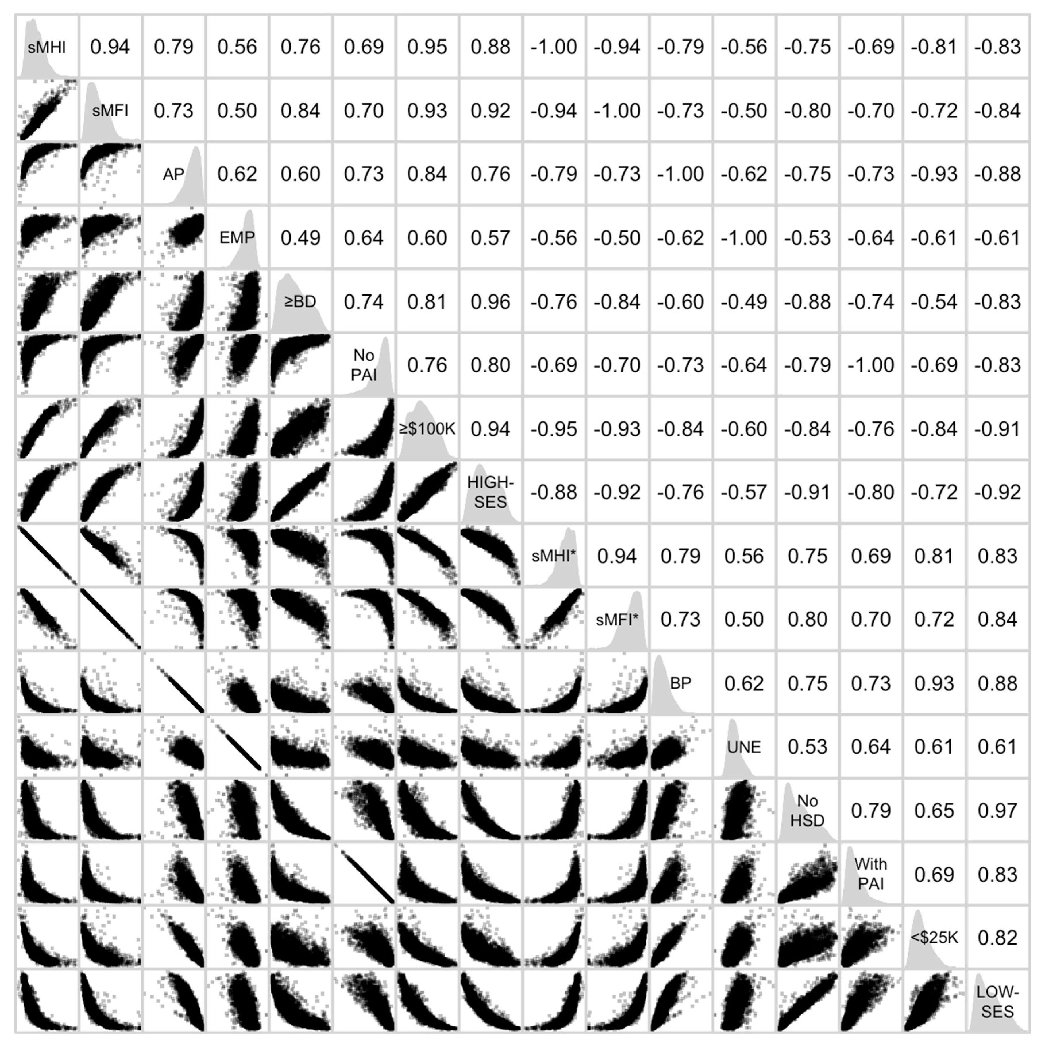
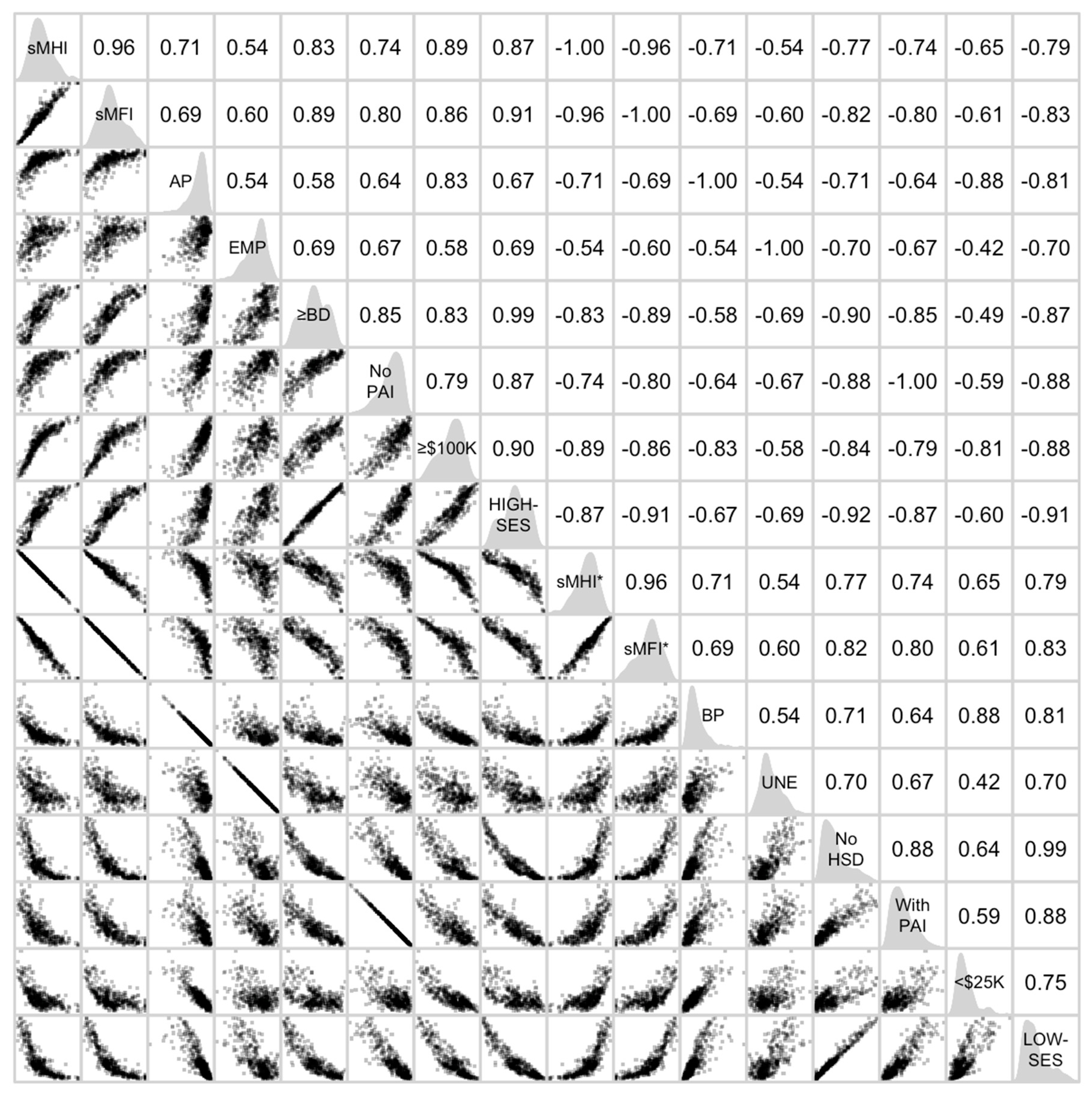
As shown in Figure 1, Figure 2, Figure 3, Figure 4, Figure 5, Figure 6 and Figure 7, sMHI and sMFI were very strongly and positively correlated with each other following a linear pattern with a small dispersion (0.91 ≤ r ≤ 0.96) and sMHI* and sMFI* were very strongly and positively correlated with each other following a linear pattern with a small dispersion (0.91 ≤ r ≤ 0.96). Since two reference measures were divided or multiplied by −1 to obtain their reversed form, sMHI and sMHI* as well as sMFI and sMFI* were perfectly and negatively correlated with each other (r = −1.00). Between five spatial high-SES indicators and their respective low-SES counterparts, perfect negative correlations (r = −1.00) were also evident between AP (above poverty) and BP (below poverty), EMP (employed) and UNE (unemployed), and NoPAI (no public assistance income) and WithPAI (with public assistance income). However, ≥BD (bachelor’s degree or higher) and NoHSD (no high school diploma) as well as ≥$100K (household income greater than or equal to USD 100,000) and <$25K (household income less than USD 25,000) were strongly, but negatively correlated with each other following a curvilinear pattern with a moderate dispersion (−0.80 ≤ r ≤ −0.85). While the forms and strengths of these relationships somewhat varied at four different time periods, very similar relationships were observed in correlation matrices based on the 2000 Census data as well as the 2005–2009 and 2010–2014 ACS data (Figures S1–S21).

Table 5. Overall percentages of high and low socioeconomic groups and component loadings of spatial high- and low-SES indicators in the Riverside–San Bernardino–Ontario Metropolitan Statistical Area (MSA).

		Overall Percentages
a		2000	2005–2009	2010–2014	2015–2019
High Socioeconomic Groups
	Above Poverty	84.95%	86.72%	82.03%	85.24%
	Employed	92.06%	90.69%	85.87%	92.44%
	Bachelor’s Degree or Higher	16.27%	19.31%	19.82%	21.69%
	No Public Assistance Income	94.58%	96.45%	95.17%	96.14%
	Household Income ≥ USD 100,000	11.54%	22.89%	23.13%	30.26%
Low Socioeconomic Groups
	Below Poverty	15.05%	13.28%	17.97%	14.76%
	Unemployed	7.94%	9.31%	14.13%	7.56%
	No High School Diploma	25.43%	21.83%	20.91%	18.91%
	With Public Assistance Income	5.42%	3.55%	4.83%	3.86%
	Household Income < USD 25,000	28.42%	20.04%	21.78%	17.99%
		Component Loadings
b		2000	2005–2009	2010–2014	2015–2019
Spatial High-SES Indicators
	Above Poverty (AP)	0.50390	0.38845	0.44687	0.35073
	Employed (EMP)	0.19125	0.12161	0.17112	0.10936
	Bachelor’s Degree or Higher (≥BD)	0.62245	0.54135	0.54816	0.55131
	No Public Assistance Income (NoPAI)	0.21893	0.12265	0.14252	0.09325
	Household Income ≥ USD 100,000 (≥$100K)	0.52358	0.72541	0.67099	0.74323
Spatial Low-SES Indicators
	Below Poverty (BP)	0.44414	0.46381	0.52371	0.49592
	Unemployed (UNE)	0.15221	0.13453	0.18541	0.14188
	No High School Diploma (NoHSD)	0.62145	0.68256	0.65206	0.65365
	With Public Assistance Income (WithPAI)	0.17360	0.14020	0.16269	0.12088
	Household Income < USD 25,000 (<$25K)	0.60270	0.53031	0.48960	0.54043

Note: Five spatial high-SES indicators and their respective low-SES counterparts refer to the composite proportion of socioeconomic groups (see Equations (1) and (2)). Abbreviation: SES, Socioeconomic Status.

Table 6. Overall percentages of high and low socioeconomic groups and component loadings of spatial high- and low-SES indicators in the San Diego–Chula Vista–Carlsbad Metropolitan Statistical Area (MSA).

		Overall Percentages
a		2000	2005–2009	2010–2014	2015–2019
High Socioeconomic Groups
	Above Poverty	87.57%	88.46%	85.31%	88.41%
	Employed	94.07%	93.27%	90.41%	94.00%
	Bachelor’s Degree or Higher	29.52%	34.01%	35.10%	38.81%
	No Public Assistance Income	96.43%	97.80%	97.24%	97.59%
	Household Income ≥ USD 100,000	15.71%	28.41%	30.22%	39.17%
Low Socioeconomic Groups
	Below Poverty	12.43%	11.54%	14.69%	11.59%
	Unemployed	5.93%	6.73%	9.59%	6.00%
	No High School Diploma	17.42%	14.82%	14.24%	12.55%
	With Public Assistance Income	3.57%	2.20%	2.76%	2.41%
	Household Income < USD 25,000	24.32%	17.86%	18.85%	14.18%
		Component Loadings
b		2000	2005–2009	2010–2014	2015–2019
Spatial High-SES Indicators
	Above Poverty (AP)	0.28967	0.23747	0.25431	0.17429
	Employed (EMP)	0.10155	0.06750	0.11308	0.06666
	Bachelor’s Degree or Higher (≥BD)	0.79960	0.76909	0.77673	0.79620
	No Public Assistance Income (NoPAI)	0.13180	0.06906	0.07284	0.05807
	Household Income ≥ USD 100,000 (≥$100K)	0.49905	0.58548	0.56029	0.57260
Spatial Low-SES Indicators
	Below Poverty (BP)	0.41969	0.43987	0.49195	0.43498
	Unemployed (UNE)	0.12432	0.09383	0.16508	0.12344
	No High School Diploma (NoHSD)	0.65083	0.71110	0.68123	0.76661
	With Public Assistance Income (WithPAI)	0.16188	0.10879	0.11474	0.10915
	Household Income < USD 25,000 (<$25K)	0.59885	0.52935	0.50347	0.44266

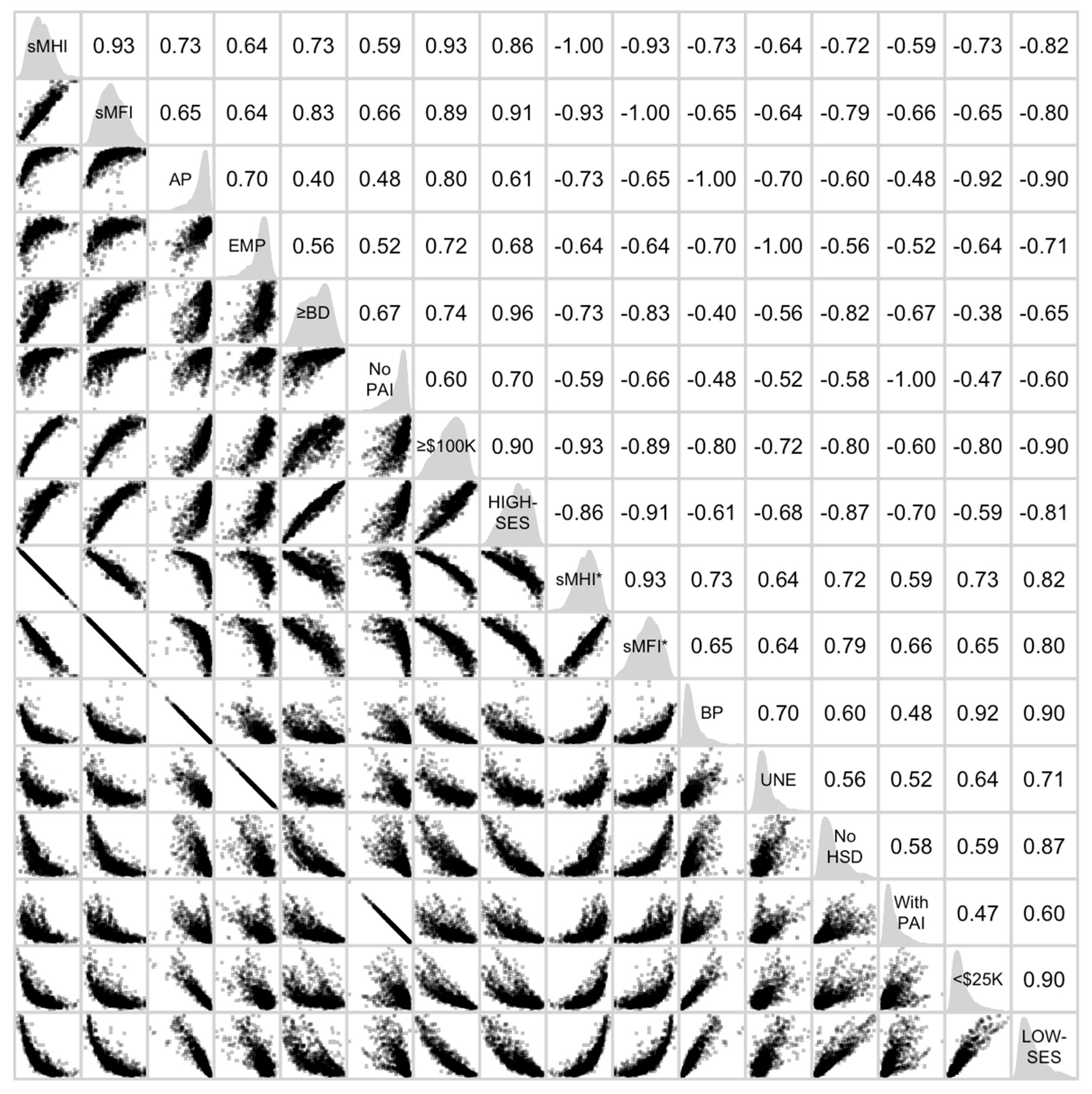
Note: Five spatial high-SES indicators and their respective low-SES counterparts refer to the composite proportion of socioeconomic groups (see Equations (1) and (2)). Abbreviation: SES, Socioeconomic Status.

By focusing on the scatterplots of pairwise relationships, Figure 1, Figure 2, Figure 3, Figure 4, Figure 5, Figure 6 and Figure 7 also show that the relationships between five spatial high-SES indicators followed positive curvilinear or nonlinear patterns with a large dispersion, although these mostly indicated moderate or strong correlations (0.23 ≤ r ≤ 0.86). On the other hand, the relationships between five spatial low-SES indicators mostly followed funnel patterns (and occasionally followed linear patterns) with a large dispersion (0.42 ≤ r ≤ 0.93). Among these indicators, ≥$100K was strongly or very strongly and positively correlated with sMHI and sMFI in a linear, but slightly curved fashion (0.86 ≤ r ≤ 0.95) and <$25K was moderately or strongly and positively correlated with sMHI* and sMFI* in a slightly curvilinear fashion (0.61 ≤ r ≤ 0.86). Since the relationships of five spatial high-SES indicators were somewhat different from those of five spatial low-SES indicators, the relationships between spatial composite measures of HIGH-SES and LOW-SES followed a strong negative curvilinear pattern with a moderate dispersion (−0.75 ≤ r ≤ −0.93). Therefore, HIGH-SES was strongly or very strongly and positively correlated with sMHI and sMFI in a linear, but slightly curved fashion (0.84 ≤ r ≤ 0.94) and LOW-SES was moderately or strongly and positively correlated with sMHI* and sMFI* in a slightly curvilinear fashion (0.75 ≤ r ≤ 0.87). While the forms and strengths of these relationships somewhat varied at four different time periods, very similar patterns were observed in correlation matrices based on the 2000 Census data as well as the 2005–2009 and 2010–2014 ACS data (Figures S1–S21).

Table 7. Overall percentages of high and low socioeconomic groups and component loadings of spatial high- and low-SES indicators in the Sacramento–Roseville–Folsom Metropolitan Statistical Area (MSA).

		Overall Percentages
a		2000	2005–2009	2010–2014	2015–2019
High Socioeconomic Groups
	Above Poverty	87.25%	88.05%	83.91%	86.60%
	Employed	93.78%	91.94%	87.99%	93.97%
	Bachelor’s Degree or Higher	26.55%	29.81%	30.70%	33.55%
	No Public Assistance Income	94.54%	95.97%	95.22%	96.23%
	Household Income ≥ USD 100,000	13.98%	25.57%	26.96%	35.28%
Low Socioeconomic Groups
	Below Poverty	12.75%	11.95%	16.09%	13.40%
	Unemployed	6.22%	8.06%	12.01%	6.03%
	No High School Diploma	15.44%	13.15%	12.02%	10.70%
	With Public Assistance Income	5.46%	4.03%	4.78%	3.77%
	Household Income < USD 25,000	24.94%	18.72%	20.60%	16.73%
		Component Loadings
b		2000	2005–2009	2010–2014	2015–2019
Spatial High-SES Indicators
	Above Poverty (AP)	0.30102	0.27132	0.34610	0.23915
	Employed (EMP)	0.12662	0.12474	0.16396	0.08385
	Bachelor’s Degree or Higher (≥BD)	0.80229	0.70715	0.67399	0.70999
	No Public Assistance Income (NoPAI)	0.22740	0.15721	0.14747	0.10983
	Household Income ≥ USD 100,000 (≥$100K)	0.44494	0.62134	0.61426	0.64779
Spatial Low-SES Indicators
	Below Poverty (BP)	0.48477	0.49715	0.59170	0.62193
	Unemployed (UNE)	0.15954	0.16282	0.19644	0.15564
	No High School Diploma (NoHSD)	0.50145	0.55552	0.47355	0.44779
	With Public Assistance Income (WithPAI)	0.22940	0.19616	0.19689	0.16399
	Household Income < USD 25,000 (<$25K)	0.65989	0.61583	0.59016	0.60130

Note: Five spatial high-SES indicators and their respective low-SES counterparts refer to the composite proportion of socioeconomic groups (see Equations (1) and (2)). Abbreviation: SES, Socioeconomic Status.

Unlike the linear or curvilinear patterns coupled with a moderate or large dispersion in the State of California and its six largest MSAs at four different time periods (Figure 1, Figure 2, Figure 3, Figure 4, Figure 5, Figure 6, Figure 7 and Figures S1–S21), linear patterns were more tightly scattered and curvilinear patterns were also more tightly scattered with a less steep curvature in the Fresno MSA (Figure 8 and 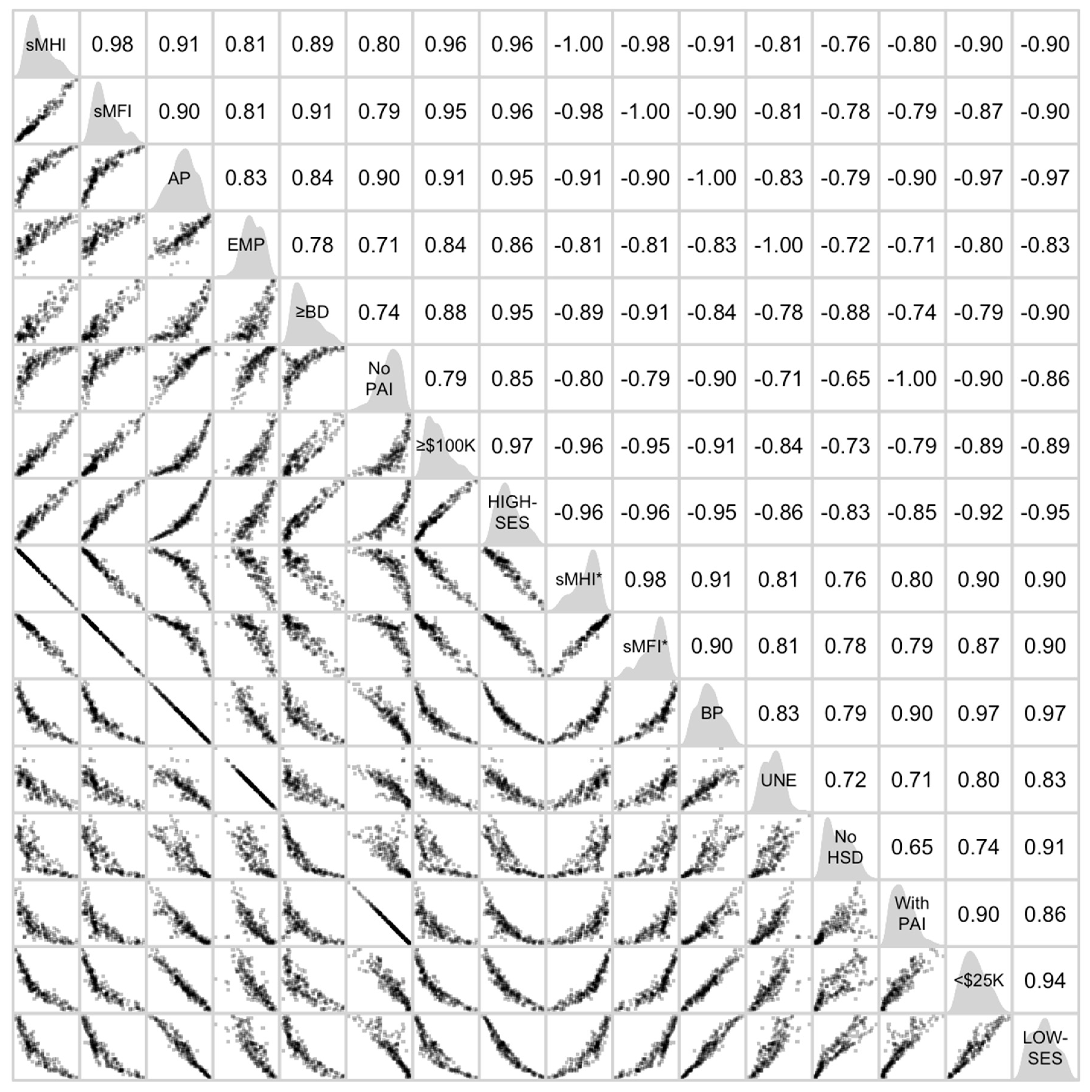Figures S22–S24). In other words, the strengths of correlations were stronger or much stronger across the board. To highlight the uniqueness of Fresno MSA, the relationships between sixteen spatial measures in the Fresno MSA (Figure 8 and Figures S22–S24) are summarized as follows.

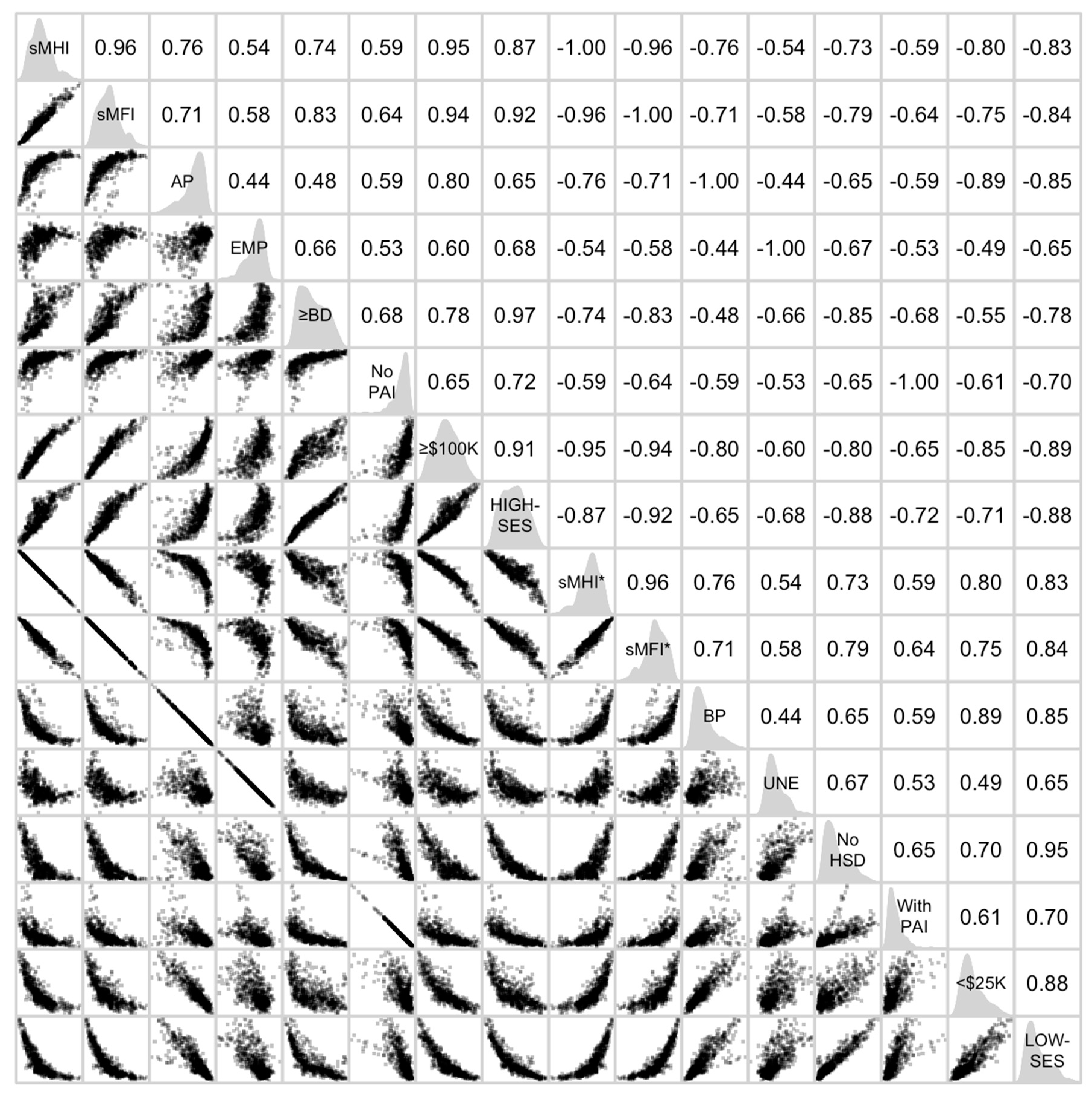
As shown in Figure 8, sMHI and sMFI (r = 0.98) as well as sMHI* and sMFI* (r = 0.98) were very strongly and positively correlated with each other following linear patterns with a very small dispersion. In addition, perfect negative correlations between sMHI and sMHI* (r = −1.00), sMFI and sMFI* (r = −1.00), AP and BP (r = −1.00), EMP and UNE (r = −1.00), and NoPAI and WithPAI (r = −1.00) remained unchanged. Moreover, ≥BD and NoHSD (r = −0.88) as well as ≥$100K and <$25K (r = −0.89) were strongly, but negatively correlated with each other following slightly curvilinear patterns with a small dispersion. Closely reflecting the tightly scattered patterns in Figure 8, almost exactly the same forms and strengths of relationships were observed in correlation matrices based on the 2000 Census data as well as the 2005–2009 and 2010–2014 ACS data (Figures S22–S24).

Table 8. Overall percentages of high and low socioeconomic groups and component loadings of spatial high- and low-SES indicators in the San Jose–Sunnyvale–Santa Clara Metropolitan Statistical Area (MSA).

		Overall Percentages
a		2000	2005–2009	2010–2014	2015–2019
High Socioeconomic Groups
	Above Poverty	92.40%	91.35%	90.00%	92.46%
	Employed	96.03%	92.95%	91.03%	95.65%
	Bachelor’s Degree or Higher	39.84%	43.16%	46.53%	51.47%
	No Public Assistance Income	97.26%	97.85%	97.50%	98.20%
	Household Income ≥ USD 100,000	34.21%	42.58%	46.89%	58.39%
Low Socioeconomic Groups
	Below Poverty	7.60%	8.65%	10.00%	7.54%
	Unemployed	3.97%	7.05%	8.97%	4.35%
	No High School Diploma	16.84%	14.54%	13.45%	11.85%
	With Public Assistance Income	2.74%	2.15%	2.50%	1.80%
	Household Income < USD 25,000	13.52%	13.61%	12.96%	9.75%
		Component Loadings
b		2000	2005–2009	2010–2014	2015–2019
Spatial High-SES Indicators
	Above Poverty (AP)	0.14408	0.16464	0.19713	0.11253
	Employed (EMP)	0.05896	0.06725	0.09337	0.03751
	Bachelor’s Degree or Higher (≥BD)	0.83869	0.82431	0.81372	0.86535
	No Public Assistance Income (NoPAI)	0.08128	0.05422	0.05012	0.04476
	Household Income ≥ USD 100,000 (≥$100K)	0.51553	0.53473	0.53644	0.48487
Spatial Low-SES Indicators
	Below Poverty (BP)	0.27501	0.34245	0.41806	0.29676
	Unemployed (UNE)	0.09646	0.11879	0.17148	0.08429
	No High School Diploma (NoHSD)	0.89104	0.84374	0.78909	0.90068
	With Public Assistance Income (WithPAI)	0.13646	0.10768	0.09239	0.09983
	Household Income < USD 25,000 (<$25K)	0.32015	0.38095	0.40574	0.28920

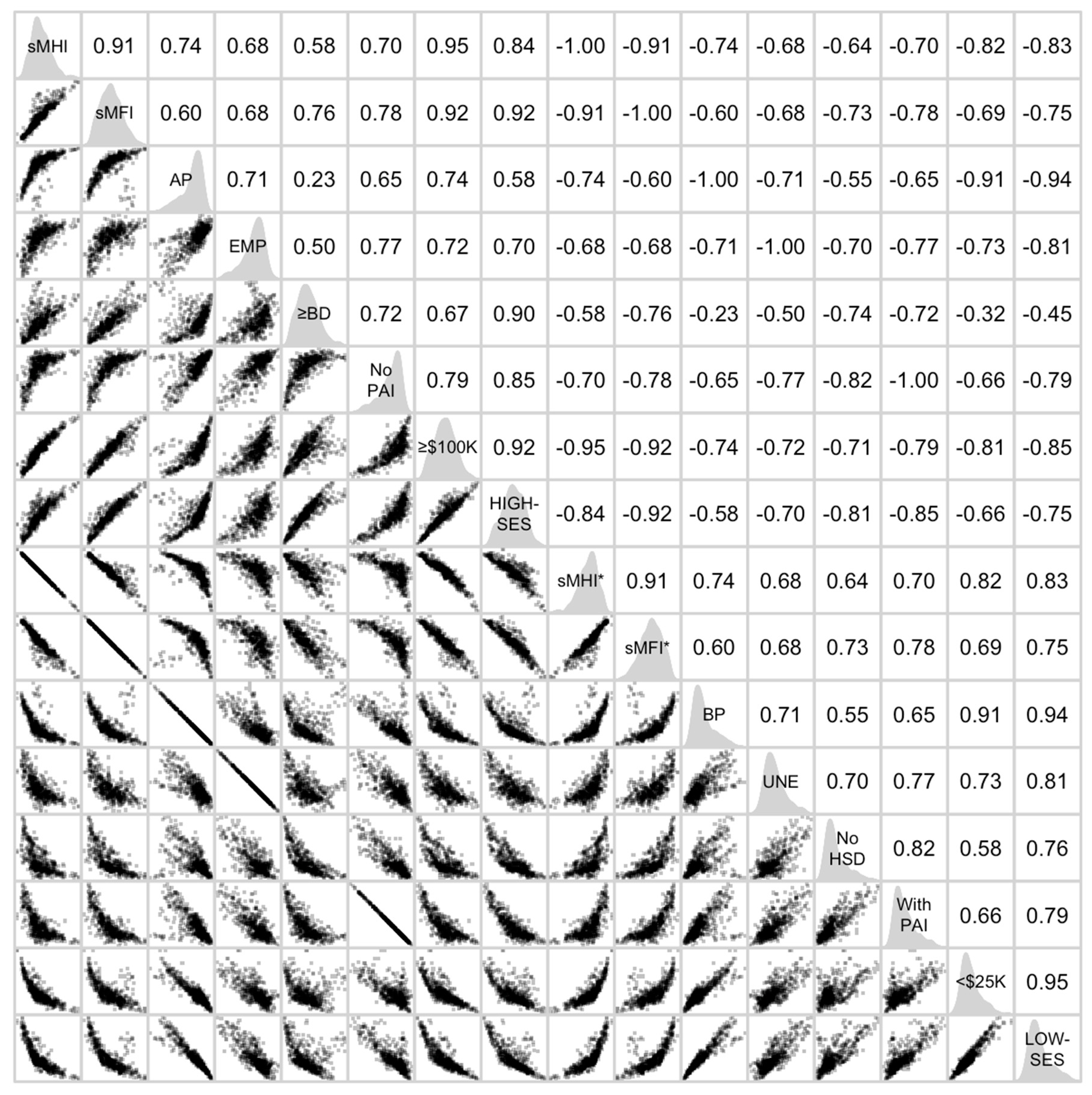
Note: Five spatial high-SES indicators and their respective low-SES counterparts refer to the composite proportion of socioeconomic groups (see Equations (1) and (2)). Abbreviation: SES, Socioeconomic Status.

Fairly different from the State of California (Figure 1) and its six largest MSAs (Figure 2, Figure 3, Figure 4, Figure 5, Figure 6 and Figure 7), five spatial high-SES indicators in Fresno MSA (Figure 8) were strongly and positively correlated with one another following linear or slightly curvilinear patterns with a small dispersion (0.71 ≤ r ≤ 0.91). Also, five spatial low-SES indicators in Fresno MSA (Figure 8) were strongly and positively correlated with one another following linear or slightly funnel patterns with a small dispersion (0.65 ≤ r ≤ 0.97). By and large, five spatial high-SES indicators were strongly and positively correlated with sMHI and sMFI in linear or slightly curvilinear fashions (0.79 ≤ r ≤ 0.96) and five spatial low-SES indicators were strongly and positively correlated with sMHI* and sMFI* in curvilinear fashions (0.76 ≤ r ≤ 0.91). While the relationships of five spatial high-SES indicators were somewhat different from those of five spatial low-SES indicators, spatial composite measures of HIGH-SES and LOW-SES were very strongly, but negatively correlated with each other following a slightly curvilinear pattern with a small dispersion (r ≤ −0.95). Moreover, HIGH-SES was very strongly and positively correlated with sMHI and sMFI in a linear fashion (r ≤ 0.96) and LOW-SES was very strongly and positively correlated with sMHI* and sMFI* in a slightly curvilinear fashion (r ≤ 0.90). Closely reflecting the tightly scattered patterns in Figure 8, almost exactly the same forms and strengths of relationships were observed in correlation matrices based on the 2000 Census data as well as the 2005–2009 and 2010–2014 ACS data (Figures S22–S24).

Table 9. Overall percentages of high and low socioeconomic groups and component loadings of spatial high- and low-SES indicators in the Fresno Metropolitan Statistical Area (MSA).

		Overall Percentages
a		2000	2005–2009	2010–2014	2015–2019
High Socioeconomic Groups
	Above Poverty	77.11%	79.08%	72.64%	77.45%
	Employed	88.19%	90.01%	85.68%	91.29%
	Bachelor’s Degree or Higher	17.55%	19.39%	19.48%	21.17%
	No Public Assistance Income	91.48%	93.57%	91.80%	92.59%
	Household Income ≥ USD 100,000	8.60%	17.36%	18.04%	24.02%
Low Socioeconomic Groups
	Below Poverty	22.89%	20.92%	27.36%	22.55%
	Unemployed	11.81%	9.99%	14.32%	8.71%
	No High School Diploma	32.48%	27.38%	26.78%	24.04%
	With Public Assistance Income	8.52%	6.43%	8.20%	7.41%
	Household Income < USD 25,000	35.96%	27.38%	28.44%	23.85%
		Component Loadings
b		2000	2005–2009	2010–2014	2015–2019
Spatial High-SES Indicators
	Above Poverty (AP)	0.62481	0.53058	0.59134	0.50281
	Employed (EMP)	0.27542	0.17498	0.15434	0.12718
	Bachelor’s Degree or Higher (≥BD)	0.59784	0.58857	0.52824	0.56584
	No Public Assistance Income (NoPAI)	0.29804	0.19907	0.21205	0.17348
	Household Income ≥ USD 100,000 (≥$100K)	0.29583	0.54938	0.54999	0.61704
Spatial Low-SES Indicators
	Below Poverty (BP)	0.47337	0.47461	0.56499	0.52519
	Unemployed (UNE)	0.21327	0.15859	0.13860	0.12739
	No High School Diploma (NoHSD)	0.64991	0.67650	0.59774	0.62326
	With Public Assistance Income (WithPAI)	0.22522	0.17784	0.20246	0.18120
	Household Income < USD 25,000 (<$25K)	0.50728	0.51021	0.51312	0.53540

Note: Five spatial high-SES indicators and their respective low-SES counterparts refer to the composite proportion of socioeconomic groups (see Equations (1) and (2)). Abbreviation: SES, Socioeconomic Status.

Regardless of the subtle differences across the study areas at four different time periods (Figure 1, Figure 2, Figure 3, Figure 4, Figure 5, Figure 6, Figure 7, Figure 8 and Figures S1–S24), consistent relationships were evident from a sequence of data analyses: sMHI and sMFI showed strong positive linear or slightly curvilinear correlations with HIGH-SES (0.73 ≤ r ≤ 0.97), sMHI* and sMFI* showed strong positive curvilinear or slightly curvilinear correlations with LOW-SES (0.72 ≤ r ≤ 0.92), and HIGH-SES and LOW-SES showed strong negative curvilinear or slightly curvilinear correlations (−0.74 ≤ r ≤ −0.98). While two spatial composite measures are conceptually inverses of each other, their relationships did not show a perfect negative linear correlation in any of the study areas at any time periods.

Figure 1. Correlation matrix of sixteen spatial measures in the State of California based on the 2015–2019 American Community Survey data. Abbreviations: SES, Socioeconomic Status; sMHI, a spatial median of median household income; sMFI, a spatial median of median family income; AP, a composite proportion of residents who were above poverty; EMP, a composite proportion of residents who were employed; ≥BD, a composite proportion of residents who held a Bachelor’s degree or higher; NoPAI, a composite proportion of residents who received no public assistance income; ≥$100K, a composite proportion of residents who earned an annual household income of greater than or equal to USD 100,000; HIGH-SES, a spatial composite measure of five spatial high-SES indicators derived from a principal component analysis; sMHI*, a spatial median of median household income divided or multiplied by −1; sMFI*, a spatial median of median family income divided or multiplied by −1; BP, a composite proportion of residents who were below poverty; UNE, a composite proportion of residents who were unemployed; NoHSD, a composite proportion of residents who had no high school diploma; WithPAI, a composite proportion of residents who were supported with public assistance income; <$25K, a composite proportion of residents who earned an annual household income of less than USD 25,000; and LOW-SES, a spatial composite measure of five spatial low-SES indicators derived from a principal component analysis.

Figure 2. Correlation matrix of sixteen spatial measures in the Los Angeles–Long Beach–Anaheim Metropolitan Statistical Area based on the 2015–2019 American Community Survey data. Abbreviations: SES, Socioeconomic Status; sMHI, a spatial median of median household income; sMFI, a spatial median of median family income; AP, a composite proportion of residents who were above poverty; EMP, a composite proportion of residents who were employed; ≥BD, a composite proportion of residents who held a Bachelor’s degree or higher; NoPAI, a composite proportion of residents who received no public assistance income; ≥$100K, a composite proportion of residents who earned an annual household income of greater than or equal to USD 100,000; HIGH-SES, a spatial composite measure of five spatial high-SES indicators derived from a principal component analysis; sMHI*, a spatial median of median household income divided or multiplied by −1; sMFI*, a spatial median of median family income divided or multiplied by −1; BP, a composite proportion of residents who were below poverty; UNE, a composite proportion of residents who were unemployed; NoHSD, a composite proportion of residents who had no high school diploma; WithPAI, a composite proportion of residents who were supported with public assistance income; <$25K, a composite proportion of residents who earned an annual household income of less than USD 25,000; and LOW-SES, a spatial composite measure of five spatial low-SES indicators derived from a principal component analysis.

Figure 3. Correlation matrix of sixteen spatial measures in the San Francisco–Oakland–Berkeley Metropolitan Statistical Area based on the 2015–2019 American Community Survey data. Abbreviations: SES, Socioeconomic Status; sMHI, a spatial median of median household income; sMFI, a spatial median of median family income; AP, a composite proportion of residents who were above poverty; EMP, a composite proportion of residents who were employed; ≥BD, a composite proportion of residents who held a Bachelor’s degree or higher; NoPAI, a composite proportion of residents who received no public assistance income; ≥$100K, a composite proportion of residents who earned an annual household income of greater than or equal to USD 100,000; HIGH-SES, a spatial composite measure of five spatial high-SES indicators derived from a principal component analysis; sMHI*, a spatial median of median household income divided or multiplied by −1; sMFI*, a spatial median of median family income divided or multiplied by −1; BP, a composite proportion of residents who were below poverty; UNE, a composite proportion of residents who were unemployed; NoHSD, a composite proportion of residents who had no high school diploma; WithPAI, a composite proportion of residents who were supported with public assistance income; <$25K, a composite proportion of residents who earned an annual household income of less than USD 25,000; and LOW-SES, a spatial composite measure of five spatial low-SES indicators derived from a principal component analysis.

Figure 4. Correlation matrix of sixteen spatial measures in the Riverside–San Bernardino–Ontario Metropolitan Statistical Area based on the 2015–2019 American Community Survey data. Abbreviations: SES, Socioeconomic Status; sMHI, a spatial median of median household income; sMFI, a spatial median of median family income; AP, a composite proportion of residents who were above poverty; EMP, a composite proportion of residents who were employed; ≥BD, a composite proportion of residents who held a Bachelor’s degree or higher; NoPAI, a composite proportion of residents who received no public assistance income; ≥$100K, a composite proportion of residents who earned an annual household income of greater than or equal to USD 100,000; HIGH-SES, a spatial composite measure of five spatial high-SES indicators derived from a principal component analysis; sMHI*, a spatial median of median household income divided or multiplied by −1; sMFI*, a spatial median of median family income divided or multiplied by −1; BP, a composite proportion of residents who were below poverty; UNE, a composite proportion of residents who were unemployed; NoHSD, a composite proportion of residents who had no high school diploma; WithPAI, a composite proportion of residents who were supported with public assistance income; <$25K, a composite proportion of residents who earned an annual household income of less than USD 25,000; and LOW-SES, a spatial composite measure of five spatial low-SES indicators derived from a principal component analysis.

Figure 5. Correlation matrix of sixteen spatial measures in the San Diego–Chula Vista–Carlsbad Metropolitan Statistical Area based on the 2015–2019 American Community Survey data. Abbreviations: SES, Socioeconomic Status; sMHI, a spatial median of median household income; sMFI, a spatial median of median family income; AP, a composite proportion of residents who were above poverty; EMP, a composite proportion of residents who were employed; ≥BD, a composite proportion of residents who held a Bachelor’s degree or higher; NoPAI, a composite proportion of residents who received no public assistance income; ≥$100K, a composite proportion of residents who earned an annual household income of greater than or equal to USD 100,000; HIGH-SES, a spatial composite measure of five spatial high-SES indicators derived from a principal component analysis; sMHI*, a spatial median of median household income divided or multiplied by −1; sMFI*, a spatial median of median family income divided or multiplied by −1; BP, a composite proportion of residents who were below poverty; UNE, a composite proportion of residents who were unemployed; NoHSD, a composite proportion of residents who had no high school diploma; WithPAI, a composite proportion of residents who were supported with public assistance income; <$25K, a composite proportion of residents who earned an annual household income of less than USD 25,000; and LOW-SES, a spatial composite measure of five spatial low-SES indicators derived from a principal component analysis.

Figure 6. Correlation matrix of sixteen spatial measures in the Sacramento–Roseville–Folsom Metropolitan Statistical Area based on the 2015–2019 American Community Survey data. Abbreviations: SES, Socioeconomic Status; sMHI, a spatial median of median household income; sMFI, a spatial median of median family income; AP, a composite proportion of residents who were above poverty; EMP, a composite proportion of residents who were employed; ≥BD, a composite proportion of residents who held a Bachelor’s degree or higher; NoPAI, a composite proportion of residents who received no public assistance income; ≥$100K, a composite proportion of residents who earned an annual household income of greater than or equal to USD 100,000; HIGH-SES, a spatial composite measure of five spatial high-SES indicators derived from a principal component analysis; sMHI*, a spatial median of median household income divided or multiplied by −1; sMFI*, a spatial median of median family income divided or multiplied by −1; BP, a composite proportion of residents who were below poverty; UNE, a composite proportion of residents who were unemployed; NoHSD, a composite proportion of residents who had no high school diploma; WithPAI, a composite proportion of residents who were supported with public assistance income; <$25K, a composite proportion of residents who earned an annual household income of less than USD 25,000; and LOW-SES, a spatial composite measure of five spatial low-SES indicators derived from a principal component analysis.

Figure 7. Correlation matrix of sixteen spatial measures in the San Jose–Sunnyvale–Santa Clara Metropolitan Statistical Area based on the 2015–2019 American Community Survey data. Abbreviations: SES, Socioeconomic Status; sMHI, a spatial median of median household income; sMFI, a spatial median of median family income; AP, a composite proportion of residents who were above poverty; EMP, a composite proportion of residents who were employed; ≥BD, a composite proportion of residents who held a Bachelor’s degree or higher; NoPAI, a composite proportion of residents who received no public assistance income; ≥$100K, a composite proportion of residents who earned an annual household income of greater than or equal to USD 100,000; HIGH-SES, a spatial composite measure of five spatial high-SES indicators derived from a principal component analysis; sMHI*, a spatial median of median household income divided or multiplied by −1; sMFI*, a spatial median of median family income divided or multiplied by −1; BP, a composite proportion of residents who were below poverty; UNE, a composite proportion of residents who were unemployed; NoHSD, a composite proportion of residents who had no high school diploma; WithPAI, a composite proportion of residents who were supported with public assistance income; <$25K, a composite proportion of residents who earned an annual household income of less than USD 25,000; and LOW-SES, a spatial composite measure of five spatial low-SES indicators derived from a principal component analysis.

Figure 8. Correlation matrix of sixteen spatial measures in the Fresno Metropolitan Statistical Area based on the 2015–2019 American Community Survey data. Abbreviations: SES, Socioeconomic Status; sMHI, a spatial median of median household income; sMFI, a spatial median of median family income; AP, a composite proportion of residents who were above poverty; EMP, a composite proportion of residents who were employed; ≥BD, a composite proportion of residents who held a Bachelor’s degree or higher; NoPAI, a composite proportion of residents who received no public assistance income; ≥$100K, a composite proportion of residents who earned an annual household income of greater than or equal to USD 100,000; HIGH-SES, a spatial composite measure of five spatial high-SES indicators derived from a principal component analysis; sMHI*, a spatial median of median household income divided or multiplied by −1; sMFI*, a spatial median of median family income divided or multiplied by −1; BP, a composite proportion of residents who were below poverty; UNE, a composite proportion of residents who were unemployed; NoHSD, a composite proportion of residents who had no high school diploma; WithPAI, a composite proportion of residents who were supported with public assistance income; <$25K, a composite proportion of residents who earned an annual household income of less than USD 25,000; and LOW-SES, a spatial composite measure of five spatial low-SES indicators derived from a principal component analysis.

5. Discussion

The results of this study (Figure 1, Figure 2, Figure 3, Figure 4, Figure 5, Figure 6, Figure 7, Figure 8 and Figures S1–S24) did not support a general notion of exchangeability between two sets of mutually opposite census-tract-level SES indicators. Because such a notion plays an essential role in the development of an area-based index and thus the measurement of neighborhood-level SES, a convoluted manifestation of curvilinear, funnel, and nonlinear patterns, in turn, calls for a thorough assessment on the measurement validity of existing area-based indices used in the US (and other countries). In addition, two spatial approaches (Oka and Wong 2016; Wong 1998) implemented in this study suggest that the measurement uncertainty of existing area-based indices may be attributed largely to the shape of their multivariate distribution and partly to their aspatial nature. From a measurement perspective, a sequence of correlation analyses conducted in an array of geographic ranges and their demographic changes at four different time periods (Figure 1, Figure 2, Figure 3, Figure 4, Figure 5, Figure 6, Figure 7, Figure 8 and Figures S1–S24) provide a reasonable basis to untangle a few underlying sources of measurement uncertainty overlooked by Allik et al. (2020) and Sorice et al. (2022).

Whether misled or obscured by the dearth of analytical transparency in the literature, the complexities of human geography (O’Sullivan 2004) and geographies of uncertainty (Senanayake and King 2021) have been largely overlooked during the development process of existing area-based indices in the US (and in other countries). In all likelihood, an oversight of such complexities may give rise to measurement error in different geographic settings. For instance, a sequence of correlation analyses in the State of California (Figure 1 and Figures S1–S3) and its six largest MSAs (Figure 2, Figure 3, Figure 4, Figure 5, Figure 6 and Figure 7 and Figures S4–S21) suggest that a set of census-tract-level SES indicators may not intercorrelate with one another and thus a conceptualization of high-SES neighborhoods may not invert to a conceptualization of low-SES neighborhoods (or vice versa). The only exception was the Fresno MSA (Figure 8 and Figures S22–S24), which comprised about 800,000 to about 985,000 people and 158 or 199 census tracts (Table 1). While the population size of one million and/or the sample size of 200 census tracts may not be considered as a differential threshold, the measurement uncertainty (Allik et al. 2020; Sorice et al. 2022) may be greater in large geographic ranges (e.g., large MSAs and states) and lesser in small geographic ranges (e.g., cities and small MSAs). Therefore, the measurement uncertainty (Allik et al. 2020; Sorice et al. 2022) may arise from a difference in the size of human settlements that vary in geographic space.

Since the generalizability of existing area-based indices has not been elucidated in a clear and straightforward manner, further efforts are needed to assess their measurement validity by ensuring an exchangeability between two sets of mutually opposite census-tract-level SES indicators in a wide array of geographic ranges (e.g., from a city to a MSA to a combination of nearby MSAs and its peripheral counties to an entire state and then to the entire conterminous US). Otherwise, an area-based index may not capture what it is intended to capture (i.e., a change from highest to lowest SES neighborhoods or vice versa). In doing so, however, it is important to recognize that distributional patterns of socioeconomic groups tend to be complex and dynamic thereby exhibiting noticeable differences between urban, suburban, and rural areas in the US (Parker et al. 2018). By and large, these differences reflect local and regional variations in the economic growth and decline of the US (Cromartie 2018; Johnson 2012). While conceptual and methodological approaches to the measurement of neighborhood-level SES have long been centered around a multifactorial construct of multiple census-tract-level SES indicators (Allik et al. 2020; Sorice et al. 2022), such a construct may be applicable to certain geographic settings, but may not be generalizable to other geographic settings. Therefore, the measurement uncertainty (Allik et al. 2020; Sorice et al. 2022) may arise from an intertwined interplay of residential preferences (Parker et al. 2018) and economic opportunities (Cromartie 2018; Johnson 2012) that vary in geographic space.

In conjunction with urban–suburban–rural variations in the size of human settlements and the socioeconomic makeup of neighborhoods, the quality of population estimates (United States Census Bureau 2020) and the outlier-prone nature of multivariate techniques (Chesher 1991) cast additional layers of uncertainty over a conventional multivariate approach to the measurement of neighborhood-level SES. On the whole, population estimates at the census tract level (but more so at the block group level) tend to be less accurate (with relatively large margins of error) in sparsely populated areas relative to those in densely populated areas (Bazuin and Fraser 2013; Folch et al. 2016; Spielman et al. 2014). Independent from the accuracy of population estimates, one or more multivariate outliers may emerge from any multivariate technique even in the absence of a univariate outlier (Hair et al. 2009) and addressing this computational problem may not be a trivial task (Aggarwal 2013) depending on the dataset being analyzed. While these have been widely regarded as unavoidable sources of measurement error, a comparative study of two similar aspatial composite measures of neighborhood-level SES (Boscoe et al. 2021) showed substantial dissimilarities between the two in different parts of the US, particularly in local areas with missing data and multivariate outliers. Therefore, the measurement uncertainty (Allik et al. 2020; Sorice et al. 2022) may arise from the presence of missing data and/or multivariate outlier(s) that vary in geographic space.

Given the complexities of human geography (O’Sullivan 2004) and geographies of uncertainty (Senanayake and King 2021), only a few underlying sources of measurement uncertainty overlooked by Allik et al. (2020) and Sorice et al. (2022) were described in this study. However, these closely coincide with a couple of common oversights masked by the lack of analytical transparency on the exploratory data analysis of existing area-based indices in the US (and in other countries). As a consequence of such oversights, for example, the curvilinear relationships between HIGH-SES and LOW-SES with a moderate or large dispersion in the State of California and its six largest MSAs at four different time periods (Figure 1, Figure 2, Figure 3, Figure 4, Figure 5, Figure 6, Figure 7 and Figures S1–S21) suggest high degrees of measurement uncertainty, whereas the slightly curvilinear relationships between HIGH-SES and LOW-SES with a small dispersion in the Fresno MSA at four different time periods (Figure 8 and Figures S22–S24) suggest low degrees of measurement uncertainty. While Allik et al. (2020) and Sorice et al. (2022) emphasized the importance of reaching a consensus on the conceptual and methodological approach to the measurement of neighborhood-level SES, the complexities of human geography (O’Sullivan 2004) and geographies of uncertainty (Senanayake and King 2021) may pose unprecedented challenges for such research endeavors. Taken together, further efforts on the development of a reliable area-based index in the US (and in other countries) may require a refined conceptualization of neighborhood-level SES and a more sophisticated method to measure it.

By virtue of the study design, a detailed assessment on the measurement validity (Bannigan and Watson 2009; Bartlett and Frost 2008; Heale and Twycross 2015) was beyond the scope of this study. However, a combination of Pearson’s correlation coefficients and scatterplots shown in Figure 1, Figure 2, Figure 3, Figure 4, Figure 5, Figure 6, Figure 7, Figure 8 and Figures S1–S24 reconfirms the usefulness of explanatory data analysis in understanding the aptness of a hypothetical area-based index used in this study. Notwithstanding the descriptive nature of a correlogram (Friendly 2002), conducting research on analytical transparency in this way may prevent, reduce, or mitigate the inconsistency of research findings (Allik et al. 2020; Sorice et al. 2022) in different geographic settings. Whether modifying an existing area-based index or developing a new one, therefore, further efforts on the development of a reliable area-based index needs to demonstrate its reliability by capturing a change from highest to lowest SES neighborhoods and a change from lowest to highest SES neighborhoods in an inverse manner (at least, equivalent to the relationships between HIGH-SES and LOW-SES shown in Figure 8 and Figures S22–S24). Since the lack of analytical transparency may have been responsible for some aspects of the measurement uncertainty (Allik et al. 2020; Sorice et al. 2022), further efforts need to pay utmost attention to detail for avoiding ambiguity, confusion, and misunderstandings.

The preceding discussions on a few underlying sources of measurement uncertainty inherent in existing area-based indices and on further efforts in developing a reliable area-based index are not only relevant to the State of California, but also to other states and to the entire US. Since the study of neighborhoods and health has been conducted mostly in industrialized countries, the same notion of analogy applies to non-US countries. Even if the size of small enumeration units were to be slightly smaller or larger than that of census tracts in the US, the concepts of composite population (Wong 1998) and areal median filtering (Oka and Wong 2016) can be implemented in other countries. However, the design of census questionnaires differs considerably from one country to another and thus a set of spatial high-SES indicators and their respective low-SES counterparts may be restricted to the availability of census data in their own country. In view of the unavoidable reality of such inter-country differences, a consensus on the optimal number and types of census-tract-level SES indicators incorporated into an area-based index (Allik et al. 2020; Sorice et al. 2022) is of importance only within a country, but not between or across countries. Hence, further efforts need to focus on the development of a reliable area-based index based on the available census data at hand and to ensure its measurement validity across a wide array of geographic ranges and their demographic changes at different time periods in their own country.

6. Conclusions

Grounded in the variety of geographic characteristics and population sizes (Table 1) considered in this study and the concepts of composite population (Wong 1998) and areal median filtering (Oka and Wong 2016) used to compute spatial measures Equations (1)–(3) across the study areas, a sequence of correlation analyses in the State of California (Figure 1 and Figures S1–S3) and its seven MSAs (Figure 2, Figure 3, Figure 4, Figure 5, Figure 6, Figure 7, Figure 8 and Figures S4–S24) collectively suggest that a conventional multivariate approach to the measurement of neighborhood-level SES (Allik et al. 2020; Sorice et al. 2022) may be susceptible to the complexities of human geography (O’Sullivan 2004) and geographies of uncertainty (Senanayake and King 2021) in the US (and other counties). Despite the descriptive nature of a correlogram (Friendly 2002), the results of this study call into question the general notion of exchangeability between two sets of mutually opposite census-tract-level SES indicators postulated in existing area-based indices. Put differently, a set of census-tract-level high-SES indicators and another set of their respective low-SES counterparts incorporated into an area-based index has been presumed to produce two separate composite measures that are inverses of each other, but such a presumption may hold true only in small geographic ranges (e.g., cities and small MSAs), not in large geographic ranges (e.g., large MSAs and states).

With a vested interest in the development of a reliable area-based index in the US (Phillips et al. 2016), further efforts on the measurement validity (Bannigan and Watson 2009; Bartlett and Frost 2008; Heale and Twycross 2015) may hold the key to foster an informative research and effective dissemination of research findings for policymakers (e.g., assess community needs, allocate resources, and evaluate policy impact). However, the measurement uncertainty may arise not only from the lack of consensus on the optimal number and types of census-tract-level SES indicators incorporated into an area-based index (Allik et al. 2020; Sorice et al. 2022), but also from a few underlying sources of measurement uncertainty ascribed to the complexities of human geography (O’Sullivan 2004) and geographies of uncertainty (Senanayake and King 2021) that vary in geographic space. Since different combinations of census-tract-level SES indicators have been shown to yield substantial dissimilarities between two aspatial composite measures of neighborhood-level SES (Boscoe et al. 2021), the conceptual and methodological concerns over the measurement uncertainty pointed out by Allik et al. (2020) and Sorice et al. (2022) may be much more complicated than what they had anticipated. In other words, further efforts on the development of a reliable area-based index may require a refined conceptualization of neighborhood-level SES and a more sophisticated method to measure it. Regardless of the difficulty of such challenges, a critical aspect to the development of a reliable area-based index would be to ensure its measurement validity across a wide array of geographic ranges and their demographic changes at different time periods.

Research implications highlighted and discussed so far have focused mainly on examining the contextual effect of neighborhood-level SES on health in the US. Nonetheless, the conceptual and methodological concerns raised by Allik et al. (2020) and Sorice et al. (2022) apply, by analogy, to existing area-based indices used in other countries, such as Canada (e.g., Pampalon et al. 2009; Pampalon and Raymond 2000), Denmark (e.g., Meijer et al. 2013; Pedersen and Vedsted 2014), France (e.g., Havard et al. 2008; Pornet et al. 2012), New Zealand (Salmond et al. 1998; Salmond and Crampton 2012), Spain (e.g., Benach and Yasui 1999; Domínguez-Berjón et al. 2008), Sweden (e.g., Bajekal et al. 1996; Sariaslan et al. 2013), and the United Kingdom (e.g., Carstairs and Morris 1989; Townsend et al. 1988). Since the lack of analytical transparency may be responsible for the inconsistency of research findings (Allik et al. 2020; Sorice et al. 2022), a figure or an appendix demonstrating the aptness of an area-based index, such as a correlogram (Friendly 2002) considered in this study, needs to be fully disclosed not only in the development of an area-based index, but also in its applications across a wide array of geographic ranges and their demographic changes at different time periods. From a research communication perspective, a collective effort focused on analytical transparency is likely to foster informative research and effective dissemination of research findings for policymakers within a country and across countries.

Supplementary Materials

The following supporting information can be downloaded at: https://www.mdpi.com/article/10.3390/socsci13120693/s1, Figure S1. Correlation matrix of sixteen spatial measures in the State of California based on the 2000 Census data; Figure S2. Correlation matrix of sixteen spatial measures in the State of California based on the 2005–2009 American Community Survey data; Figure S3. Correlation matrix of sixteen spatial measures in the State of California based on the 2010–2014 American Community Survey data; Figure S4. Correlation matrix of sixteen spatial measures in the Los Angeles-Long Beach-Anaheim Metropolitan Statistical Area based on the 2000 Census data; Figure S5. Correlation matrix of sixteen spatial measures in the Los Angeles-Long Beach-Anaheim Metropolitan Statistical Area based on the 2005–2009 American Community Survey data; Figure S6. Correlation matrix of sixteen spatial measures in the Los Angeles-Long Beach-Anaheim Metropolitan Statistical Area based on the 2010–2014 American Community Survey data; Figure S7. Correlation matrix of sixteen spatial measures in the San Francisco-Oakland-Berkeley Metropolitan Statistical Area based on the 2000 Census data; Figure S8. Correlation matrix of sixteen spatial measures in the San Francisco-Oakland-Berkeley Metropolitan Statistical Area based on the 2005–2009 American Community Survey data; Figure S9. Correlation matrix of sixteen spatial measures in the San Francisco-Oakland-Berkeley Metropolitan Statistical Area based on the 2010–2014 American Community Survey data; Figure S10. Correlation matrix of sixteen spatial measures in the Riverside-San Bernardino-Ontario Metropolitan Statistical Area based on the 2000 Census data; Figure S11. Correlation matrix of sixteen spatial measures in the Riverside-San Bernardino-Ontario Metropolitan Statistical Area based on the 2005–2009 American Community Survey data; Figure S12. Correlation matrix of sixteen spatial measures in the Riverside-San Bernardino-Ontario Metropolitan Statistical Area based on the 2010–2014 American Community Survey data; Figure S13. Correlation matrix of sixteen spatial measures in the San Diego-Chula Vista-Carlsbad Metropolitan Statistical Area based on the 2000 Census data; Figure S14. Correlation matrix of sixteen spatial measures in the San Diego-Chula Vista-Carlsbad Metropolitan Statistical Area based on the 2005–2009 American Community Survey data; Figure S15. Correlation matrix of sixteen spatial measures in the San Diego-Chula Vista-Carlsbad Metropolitan Statistical Area based on the 2010–2014 American Community Survey data; Figure S16. Correlation matrix of sixteen spatial measures in the Sacramento-Roseville-Folsom Metropolitan Statistical Area based on the 2000 Census data; Figure S17. Correlation matrix of sixteen spatial measures in the Sacramento-Roseville-Folsom Metropolitan Statistical Area based on the 2005–2009 American Community Survey data; Figure S18. Correlation matrix of sixteen spatial measures s in the Sacramento-Roseville-Folsom Metropolitan Statistical Area based on the 2010–2014 American Community Survey data; Figure S19. Correlation matrix of sixteen spatial measures in the San Jose-Sunnyvale-Santa Clara Metropolitan Statistical Area based on the 2000 Census data; Figure S20. Correlation matrix of sixteen spatial measures in the San Jose-Sunnyvale-Santa Clara Metropolitan Statistical Area based on the 2005–2009 American Community Survey data; Figure S21. Correlation matrix of sixteen spatial measures in the San Jose-Sunnyvale-Santa Clara Metropolitan Statistical Area based on the 2010–2014 American Community Survey data; Figure S22. Correlation matrix of sixteen spatial measures in the Fresno Metropolitan Statistical Area based on the 2000 Census data; Figure S23. Correlation matrix of sixteen spatial measures in the Fresno Metropolitan Statistical Area based on the 2005–2009 American Community Survey data; Figure S24. Correlation matrix of sixteen spatial measures in the Fresno Metropolitan Statistical Area based on the 2010–2014 American Community Survey data.

Funding

This research received no external funding.

Institutional Review Board Statement

Not applicable.

Informed Consent Statement

Not applicable.

Data Availability Statement

Publicly available datasets analyzed in this study can be downloaded from the United States Census Bureau’s website: https://www.census.gov/data.html; (accessed on 5 June 2024).

Conflicts of Interest

The author declares no conflict of interest.

References

Aggarwal, Charu C. 2013. Outlier Analysis. New York: Springer Science + Business Media, LLC. [Google Scholar]
Allik, Mirjam, Alastair Leyland, Maria Yury Travassos Ichihara, and Ruth Dundas. 2020. Creating small-area deprivation indices: A guide for stages and options. Journal of Epidemiology and Community Health 74: 20–25. [Google Scholar] [CrossRef] [PubMed]
Anselin, Luc. 1995. Local indicators of spatial association–LISA. Geographical Analysis 27: 93–115. [Google Scholar] [CrossRef]
Arcaya, Mariana C., Reginald D. Tucker-Seeley, Rockli Kim, Alina Schnake-Mahl, Marvin So, and S. V. Subramanian. 2016. Research on neighborhood effects on health in the United States: A systematic review of study characteristics. Social Science & Medicine 168: 16–29. [Google Scholar] [CrossRef]
Bajekal, Madhavi, Sundquist Jan, and Brian Jarman. 1996. The Swedish UPA score: An administrative tool for identification of underprivileged areas. Scandinavian Journal of Social Medicine 24: 177–84. [Google Scholar] [CrossRef]
Bannigan, Katrina, and Roger Watson. 2009. Reliability and validity in a nutshell. Journal of Clinical Nursing 18: 3237–43. [Google Scholar] [CrossRef] [PubMed]
Barrett, Frank A. 1993. A medical geographical anniversary. Social Science & Medicine 47: 701–10. [Google Scholar] [CrossRef]
Barrett, Frank A. 1996. Daniel drake’s medical geography. Social Science & Medicine 42: 791–800. [Google Scholar] [CrossRef]
Barrett, Frank A. 2000. Finke’s 1792 map of human diseases: The first world disease map? Social Science & Medicine 50: 915–21. [Google Scholar] [CrossRef]
Bartlett, Jonathan W., and Chris Frost. 2008. Reliability, repeatability and reproducibility: Analysis of measurement errors in continuous variables. Ultrasound in Obstetrics and Gynecology 31: 466–75. [Google Scholar] [CrossRef]
Basta, Luke A., Therese S. Richmond, and Douglas J. Wiebe. 2010. Neighborhoods, daily activities, and measuring health risks experienced in urban environments. Social Science & Medicine 71: 1943–50. [Google Scholar] [CrossRef]
Bazuin, Joshua Theodore, and James Curtis Fraser. 2013. How the ACS gets it wrong: The story of the American community survey and a small, inner city neighborhood. Applied Geography 45: 292–302. [Google Scholar] [CrossRef]
Benach, Joan, and Yutaka Yasui. 1999. Geographical patterns of excess mortality in Spain explained by two indices of deprivation. Journal of Epidemiology and Community Health 53: 423–31. [Google Scholar] [CrossRef] [PubMed]
Besser, Lilah M., Noreen C. McDonald, Yan Song, Walter A. Kukull, and Daniel A. Rodriguez. 2017. Neighborhood environment and cognition in older adults: A systematic review. American Journal of Preventive Medicine 53: 241–51. [Google Scholar] [CrossRef] [PubMed]
Bivand, Roger. 2023. spdep: Spatial Dependence: Weighting Schemes, Statistics [Computer Software]. Available online: https://cran.r-project.org/web/packages/spdep/index.html (accessed on 5 June 2024).
Bivand, Roger S., and David W.S. Wong. 2018. Comparing implementations of global and local indicators of spatial association. Test 27: 716–48. [Google Scholar] [CrossRef]
Black, Jennifer L., and James Macinko. 2008. Neighborhoods and obesity. Nutrition Reviews 66: 2–20. [Google Scholar] [CrossRef]
Booth, Katie M., Megan M. Pinkston, and Walker S. Poston. 2005. Obesity and the built environment. Journal of the American Dietetic Association 105: S110–S17. [Google Scholar] [CrossRef] [PubMed]
Boscoe, Francis P., Bian Liu, and Furrina Lee. 2021. A comparison of two neighborhood-level socioeconomic indexes in the United States. Spatial and Spatio-temporal Epidemiology 37: 100412. [Google Scholar] [CrossRef]
Carstairs, Vera, and Russell Morris. 1989. Deprivation: Explaining differences in mortality between Scotland and England and Wales. BMJ 299: 886–89. [Google Scholar] [CrossRef]
Chaix, Basile. 2009. Geographic life environments and coronary heart disease: A literature review, theoretical contributions, methodological updates, and a research agenda. Annual Review of Public Health 30: 81–105. [Google Scholar] [CrossRef] [PubMed]
Chesher, Andrew. 1991. The effect of measurement error. Biometrika 78: 451–62. [Google Scholar] [CrossRef]
Cromartie, John. 2018. Rural America at a Glance, 2018 Edition. Available online: https://www.ers.usda.gov/webdocs/publications/90556/eib-200.pdf?v=5899.2 (accessed on 25 September 2024).
Diez Roux, Ana V. 2016. Neighborhoods and Health: What Do We Know? What Should We Do? American Journal of Public Health 106: 430–31. [Google Scholar] [CrossRef] [PubMed]
Diez Roux, Ana V., Catarina I. Kiefe, David R. Jacobs, Jr., Mary Haan, Scott A. Jackson, F. Javier Nieto, Catherine C. Paton, and Richard Schulz. 2001. Area Characteristics and Individual-Level Socioeconomic Position Indicators in Three Population-Based Epidemiologic Studies. Annals of Epidemiology 11: 395–405. [Google Scholar] [CrossRef] [PubMed]
Domínguez-Berjón, M. Felícitas, Carme Borrell, Gemma Cano-Serral, Santiago Esnaola, Andreu Nolasco, M. Isabel Pasarín, Rebeca Ramis, Carme Saurina, and Antonio Escolar-Pujolar. 2008. Constructing a deprivation index based on census data in large Spanish cities (the MEDEA project). Gaceta Sanitaria 22: 179–87. [Google Scholar] [CrossRef] [PubMed]
Duncan, Dustin T., and Ichiro Kawachi. 2018. Neighborhoods and Health, 2nd ed. New York: Oxford University Press. [Google Scholar]
Entwisle, Barbara. 2007. Putting people into place. Demography 44: 687–703. [Google Scholar] [CrossRef]
Folch, David C., Daniel Arribas-Bel, Julia Koschinsky, and Seth E. Spielman. 2016. Spatial variation in the quality of American community survey estimates. Demography 53: 1535–54. [Google Scholar] [CrossRef] [PubMed]
Folwell, Keith. 1995. Single measures of deprivation. Journal of Epidemiology and Community Health 49: S51–S56. [Google Scholar] [CrossRef] [PubMed]
Friendly, Michael. 2002. Corrgrams: Exploratory display for correlation matrices. The American Statistician 56: 316–24. [Google Scholar] [CrossRef]
Fritz, Heather, Malcolm P. Cutchin, Jamil Gharib, Neehar Haryadi, Meet Patel, and Nandit Patel. 2020. Neighborhood characteristics and frailty: A scoping review. The Gerontologist 60: e270–e285. [Google Scholar] [CrossRef]
Gelman, Andrew, and Jennifer Hill. 2007. Data Analysis Using Regression and Multilevel/Hierarchical Models. New York: Cambridge University Press. [Google Scholar]
Getis, Arthur. 2009. Spatial weights matrices. Geographical Analysis 41: 404–10. [Google Scholar] [CrossRef]
Getis, Arthur, and J. Keith Ord. 1992. The Analysis of Spatial Association by Use of Distance Statistics. Geographical Analysis 24: 189–206. [Google Scholar] [CrossRef]
Goodchild, Michael F., and Donald G. Janelle. 2010. Toward critical spatial thinking in the social sciences and humanities. GeoJournal 75: 3–13. [Google Scholar] [CrossRef] [PubMed]
Goodchild, Michael F., Luc Anselin, Richard P. Appelbaum, and Barbara Herr Harthorn. 2000. Toward spatially integrated social science. International Regional Science Review 23: 139–59. [Google Scholar] [CrossRef]
Griffith, Daniel A. 1983. The boundary value problem in spatial statistical analysis. Journal of Regional Science 23: 377–87. [Google Scholar] [CrossRef]
Hair, Joseph F., Jr., William C. Black, Barry J. Babin, and Rolph E. Anderson. 2009. Multivariate Data Analysis, 7th ed. Upper Saddle River: Prentice Hall. [Google Scholar]
Havard, Sabrina, Séverine Deguen, Julie Bodin, Karine Louis, Olivier Laurent, and Denis Bard. 2008. A small-area index of socioeconomic deprivation to capture health inequalities in France. Social Science & Medicine 67: 2007–16. [Google Scholar] [CrossRef]
Heale, Roberta, and Alison Twycross. 2015. Validity and reliability in quantitative studies. Evidence-Based Nursing 18: 66–67. [Google Scholar] [CrossRef]
Hox, Joop, Mirjam Moerbeek, and Rens van de Schoot. 2017. Multilevel Analysis: Techniques and Applications, 3rd ed. New York: Routledge. [Google Scholar]
Johnson, Kenneth M. 2012. Rural demographic change in the new century: Slower growth, increased diversity. In The Carsey School of Public Policy at the Scholars’ Repository. Durham: Carsey School of Public Policy, University of New Hampshire. [Google Scholar] [CrossRef]
Joliffe, I. T., and B. J. T. Morgan. 1992. Principal component analysis and exploratory factor analysis. Statistical Methods in Medical Research 1: 69–95. [Google Scholar] [CrossRef] [PubMed]
Jones, Malia, and Anne R. Pebley. 2014. Redefining neighborhoods using common destinations: Social characteristics of activity spaces and home census tracts compared. Demography 51: 727–52. [Google Scholar] [CrossRef] [PubMed]
Kawachi, Ichiro, and Lisa F. Berkman. 2003. Neighborhoods and Health, 1st ed. New York: Oxford University Press. [Google Scholar]
Kim, Daniel. 2008. Blues from the neighborhood? Neighborhood characteristics and depression. Epidemiologic Reviews 30: 101–17. [Google Scholar] [CrossRef] [PubMed]
Kind, Amy J. H., Steve Jencks, Jane Brock, Menggang Yu, Christie Bartels, William Ehlenbach, Caprice Greenberg, and Maureen Smith. 2014. Neighborhood socioeconomic disadvantage and 30-day rehospitalization: A retrospective cohort study. Annals of Internal Medicine 161: 765–74. [Google Scholar] [CrossRef]
Krieger, Nancy, Jarvis T. Chen, Pamela D. Waterman, David H. Rehkopf, and S.V. Subramanian. 2003a. Race/ethnicity, gender, and monitoring socioeconomic gradients in health: A comparison of area-based socioeconomic measures—The public health disparities geocoding project. American Journal of Public Health 93: 1655–71. [Google Scholar] [CrossRef]
Krieger, Nancy, Jarvis T. Chen, Pamela D. Waterman, Mah-Jabeen Soobader, S. V. Subramanian, and Rosa Carson. 2002. Geocoding and monitoring of US socioeconomic inequalities in mortality and cancer incidence: Does the choice of area-based measure and geographic level matter? American Journal of Epidemiology 156: 471–82. [Google Scholar] [CrossRef] [PubMed]
Krieger, Nancy, Jarvis T. Chen, Pamela D. Waterman, Mah-Jabeen Soobader, S. V. Subramanian, and Rosa Carson. 2003b. Choosing area based socioeconomic measures to monitor social inequalities in low birth weight and childhood lead poisoning: The public health disparities geocoding project (US). Journal of Epidemiology and Community Health 57: 186–99. [Google Scholar] [CrossRef]
Krieger, Nancy, Pamela D. Waterman, Jarvis T. Chen, and S. V. Subramanian. 2003c. Monitoring Socioeconomic Inequalities in Sexually Transmitted Infections, Tuberculosis, and Violence: Geocoding and Choice of Area-Based Socioeconomic Measures—The Public Health Disparities Geocoding Project (US). Public Health Reports 118: 240–60. [Google Scholar] [CrossRef] [PubMed]
Logan, John R. 2012. Making a Place for Space: Spatial Thinking in Social Science. Annual Review of Sociology 38: 507–24. [Google Scholar] [CrossRef] [PubMed]
Logan, John R., Weiwei Zhang, and Hongwei Xu. 2010. Applying spatial thinking in social science research. GeoJournal 75: 15–27. [Google Scholar] [CrossRef]
Mair, C., Ana V. Diez Roux, and Sandro Galea. 2008. Are neighbourhood characteristics associated with depressive symptoms? A review of evidence. Journal of Epidemiology and Community Health 62: 940–46. [Google Scholar] [CrossRef] [PubMed]
Matthews, Stephen A., and Daniel M. Parker. 2013. Progress in Spatial Demography. Demographic Research 28: 271–312. [Google Scholar] [CrossRef]
Meijer, Mathias, Gerda Engholm, Ulrike Grittner, and Kim Bloomfield. 2013. A socioeconomic deprivation index for small areas in Denmark. Scandinavian Journal of Public Health 41: 560–69. [Google Scholar] [CrossRef]
Meijer, Mathias, Jeannette Röhl, Kim Bloomfield, and Ulrike Grittner. 2012. Do neighborhoods affect individual mortality? A systematic review and meta-analysis of multilevel studies. Social Science & Medicine 74: 1204–12. [Google Scholar] [CrossRef]
Messer, Lynne C., Barbara A. Laraia, Jay S. Kaufman, Janet Eyster, Claudia Holzman, Jennifer Culhane, Irma Elo, Jessica G. Burke, and Patricia O’Campo. 2006. The Development of a Standardized Neighborhood Deprivation Index. Journal of Urban Health 83: 1041–62. [Google Scholar] [CrossRef]
Mode, Nicolle A., Michele K. Evans, and Alan B. Zonderman. 2016. Race, Neighborhood Economic Status, Income Inequality and Mortality. PLoS ONE 11: e0154535. [Google Scholar] [CrossRef] [PubMed]
Morenoff, Jeffrey D. 2003. Neighborhood Mechanisms and the Spatial Dynamics of Birth Weight. American Journal of Sociology 108: 976–1017. [Google Scholar] [CrossRef] [PubMed]
Namin, Sima, Yuhong Zhou, Joan Neuner, and Kirsten Beyer. 2021. Neighborhood Characteristics and Cancer Survivorship: An Overview of the Current Literature on Neighborhood Landscapes and Cancer Care. International Journal of Environmental Research and Public Health 18: 7192. [Google Scholar] [CrossRef] [PubMed]
Ncube, Collette N., Daniel A. Enquobahrie, Steven M. Albert, Amy L. Herrick, and Jessica G. Burke. 2016. Association of neighborhood context with offspring risk of preterm birth and low birthweight: A systematic review and meta-analysis of population-based studies. Social Science & Medicine 153: 156–64. [Google Scholar] [CrossRef]
Oka, Masayoshi. 2015. Measuring a neighborhood affluence-deprivation continuum in urban settings: Descriptive findings from four US cities. Demographic Research 32: 1469–86. [Google Scholar] [CrossRef]
Oka, Masayoshi. 2021. Interpreting a standardized and normalized measure of neighborhood socioeconomic status for a better understanding of health differences. Archives of Public Health 79: 226. [Google Scholar] [CrossRef]
Oka, Masayoshi. 2023. Census-tract-level Median Household Income and Median Family Income Estimates: A Unidimensional Measure of Neighborhood Socioeconomic Status? International Journal of Environmental Research and Public Health 20: 211. [Google Scholar] [CrossRef] [PubMed]
Oka, Masayoshi, and David W. S. Wong. 2016. Spatializing Area-based Measures of Neighborhood Characteristics for Multilevel Regression Analyses: An Areal Median Filtering Approach. Journal of Urban Health 93: 551–71. [Google Scholar] [CrossRef] [PubMed]
O’Sullivan, David. 2004. Complexity Science and Human Geography. Transactions of the Institute of British Geographers 29: 282–95. [Google Scholar] [CrossRef]
Pampalon, Robert, and Guy Raymond. 2000. A deprivation index for health and welfare planning in Quebec. Chronic Diseases in Canada 21: 104–13. [Google Scholar]
Pampalon, Robert, Denis Hamel, Philippe Gamache, and Guy Raymond. 2009. A deprivation index for health planning in Canada. Chronic Diseases in Canada 29: 178–91. [Google Scholar] [CrossRef] [PubMed]
Parker, Kim, Juliana Horowitz, Anna Brown, Richard Fry, D’Vera Cohn, and Ruth Igielnik. 2018. What Unites and Divides Urban, Suburban and Rural Communities. Available online: https://www.pewresearch.org/social-trends/2018/05/22/demographic-and-economic-trends-in-urban-suburban-and-rural-communities/#:~:text=About%2046%20million%20Americans%20live,8%25%20growth%20in%20the%201990s (accessed on 24 July 2024).
Park, Hee Sun, René Dailey, and Daisy Lemus. 2002. The Use of Exploratory Factor Analysis and Principal Components Analysis in Communication Research. Human Communication Research 28: 562–77. [Google Scholar] [CrossRef]
Pedersen, Anette Fischer, and Peter Vedsted. 2014. Understanding the inverse care law: A register and survey-based study of patient deprivation and burnout in general practice. International Journal for Equity in Health 13: 121. [Google Scholar] [CrossRef] [PubMed]
Perchoux, Camille, Basile Chaix, Steven Cummins, and Yan Kestens. 2013. Conceptualization and measurement of environmental exposure in epidemiology: Accounting for activity space related to daily mobility. Health & Place 21: 86–93. [Google Scholar] [CrossRef]
Phillips, Robert L, Winston Liaw, Peter Crampton, Daniel J Exeter, Andrew Bazemore, Katherine Diaz Vickery, Stephen Petterson, and Mark Carrozza. 2016. How Other Countries Use Deprivation Indices-And Why The United States Desperately Needs One. Health Affairs (Millwood) 35: 1991–98. [Google Scholar] [CrossRef] [PubMed]
Pornet, Carole, Cyrille Delpierre, Olivier Dejardin, Pascale Grosclaude, Ludivine Launay, Lydia Guittet, Thierry Lang, and Guy Launoy. 2012. Construction of an adaptable European transnational ecological deprivation index: The French version. Journal of Epidemiology and Community Health 66: 982–89. [Google Scholar] [CrossRef]
Raudenbush, Stephen W., and Anthony S. Bryk. 2002. Hierarchical Linear Models: Applications and Data Analysis Methods, 2nd ed. Newbury Park: Sage Publications. [Google Scholar]
R Core Team. 2024. R: A Language and Environment for Statistical Computing. Vienna: R Foundation for Statistical Computing. [Google Scholar]
Ribeiro, Ana Isabel, Joana Amaro, Cosima Lisi, and Silvia Fraga. 2018. Neighborhood Socioeconomic Deprivation and Allostatic Load: A Scoping Review. International Journal of Environmental Research and Public Health 15: 1092. [Google Scholar] [CrossRef] [PubMed]
Salmond, Clare E., and Peter Crampton. 2012. Development of New Zealand’s deprivation index (NZDep) and its uptake as a national policy tool. Canadian Journal of Public Health 103: S7–S11. [Google Scholar] [PubMed]
Salmond, Clare, Peter Crampton, and Frances Sutton. 1998. NZDep91: A New Zealand index of deprivation. Australian and New Zealand Journal of Public Health 22: 835–37. [Google Scholar] [CrossRef]
Saltelli, Andrea. 2002. Sensitivity Analysis for Importance Assessment. Risk Analysis 22: 579–90. [Google Scholar] [CrossRef] [PubMed]
Sampson, Robert J., Stephen W. Raudenbush, and Felton Earls. 1997. Neighborhoods and Violent Crime: A Multilevel Study of Collective Efficacy. Science 277: 918–24. [Google Scholar] [CrossRef] [PubMed]
Sariaslan, Amir, Niklas Långström, Brian D’Onofrio, Johan Hallqvist, Johan Franck, and Paul Lichtenstein. 2013. The impact of neighbourhood deprivation on adolescent violent criminality and substance misuse: A longitudinal, quasi-experimental study of the total Swedish population. International Journal of Epidemiology 42: 1057–66. [Google Scholar] [CrossRef]
Schreiber, James B. 2021. Issues and recommendations for exploratory factor analysis and principal component analysis. Research in Social and Administrative Pharmacy 17: 1004–11. [Google Scholar] [CrossRef]
Senanayake, Nari, and Brian King. 2021. Geographies of uncertainty. Geoforum 123: 129–35. [Google Scholar] [CrossRef] [PubMed]
Singh, Gopal K. 2003. Area Deprivation and Widening Inequalities in US Mortality, 1969–1998. American Journal of Public Health 93: 1137–43. [Google Scholar] [CrossRef] [PubMed]
Snijders, Tom A. B., and Roel J. Bosker. 2012. Multilevel Analysis: An Introduction to Basic and Advanced Multilevel Modeling, 2nd ed. Thousand Oaks: SAGE Publications. [Google Scholar]
Sorice, Kristen A., Carolyn Y. Fang, Daniel Wiese, Angel Ortiz, Yuku Chen, Kevin A. Henry, and Shannon M. Lynch. 2022. Systematic review of neighborhood socioeconomic indices studied across the cancer control continuum. Cancer Medicine 11: 2125–44. [Google Scholar] [CrossRef] [PubMed]
Spielman, Seth E., David Folch, and Nicholas Nagle. 2014. Patterns and Causes of Uncertainty in the American Community Survey. Applied Geography 46: 147–57. [Google Scholar] [CrossRef]
Townsend, Peter, Peter Phillimore, and Alastair Beattie. 1988. Health and Deprivation: Inequality and the North. London: Croom Helm. [Google Scholar]
United States Census Bureau. 2020. Understanding and Using American Community Survey Data: What All Data Users Need to Know. Available online: https://www.census.gov/content/dam/Census/library/publications/2020/acs/acs_general_handbook_2020.pdf (accessed on 15 October 2024).
United States Census Bureau. 2022. American Community Survey and Puerto Rico Community Survey Design and Methodology; Washington: U.S. Government Publishing Office.
United States Census Bureau. 2023. About the American Community Survey. Available online: https://www.census.gov/programs-surveys/acs/about.html (accessed on 23 October 2024).
United States Census Bureau. 2024. Comparing ACS Data. Available online: https://www.census.gov/programs-surveys/acs/guidance/comparing-acs-data.html (accessed on 5 June 2024).
van Vuuren, C. Leontine, Sijmen A. Reijneveld, Marcel F. van der Wal, and Arnoud P. Verhoeff. 2014. Neighborhood socioeconomic deprivation characteristics in child (0–18 years) health studies: A review. Health & Place 29: 34–42. [Google Scholar] [CrossRef]
Vinten-Johansen, Peter, Howard Brody, Nigel Paneth, Stephen Rachman, Michael Rip, and David Zuck. 2003. Cholera, Chloroform, and the Science of Medicine: A Life of John Snow. New York: Oxford University Press. [Google Scholar]
Vos, Amber A., Anke G. Posthumus, Gouke J. Bonsel, Eric A. P. Steegers, and Semiha Denktaş. 2014. Deprived neighborhoods and adverse perinatal outcome: A systematic review and meta-analysis. Acta Obstetricia et Gynecologica Scandinavica 93: 727–40. [Google Scholar] [CrossRef]
Winkleby, Marilyn A., and Catherine Cubbin. 2003. Influence of individual and neighbourhood socioeconomic status on mortality among black, Mexican-American, and white women and men in the United States. Journal of Epidemiology and Community Health 57: 444–52. [Google Scholar] [CrossRef]
Wong, David W. S. 1998. Measuring Multiethnic Spatial Segregation. Urban Geography 19: 77–87. [Google Scholar] [CrossRef]
Wright, Kevin. 2021. Corrgram: Plot a Correlogram [Computer Software]. Available online: https://cran.r-project.org/web/packages/corrgram/index.html (accessed on 5 June 2024).
Yost, Kathleen, Carin Perkins, Richard Cohen, Cyllene Morris, and William Wright. 2001. Socioeconomic status and breast cancer incidence in California for different race/ethnic groups. Cancer Causes & Control 12: 703–11. [Google Scholar] [CrossRef]
Yu, Mandi, Zaria Tatalovich, James T. Gibson, and Kathleen A. Cronin. 2014. Using a composite index of socioeconomic status to investigate health disparities while protecting the confidentiality of cancer registry data. Cancer Causes & Control 25: 81–92. [Google Scholar] [CrossRef]
Zenk, Shannon N., Amy J. Schulz, Stephen A. Matthews, Angela Odoms-Young, JoEllen Wilbur, Lani Wegrzyn, Kevin Gibbs, Carol Braunschweig, and Carmen Stokes. 2011. Activity space environment and dietary and physical activity behaviors: A pilot study. Health & Place 17: 1150–61. [Google Scholar] [CrossRef]

Disclaimer/Publisher’s Note: The statements, opinions and data contained in all publications are solely those of the individual author(s) and contributor(s) and not of MDPI and/or the editor(s). MDPI and/or the editor(s) disclaim responsibility for any injury to people or property resulting from any ideas, methods, instructions or products referred to in the content.

© 2024 by the author. Licensee MDPI, Basel, Switzerland. This article is an open access article distributed under the terms and conditions of the Creative Commons Attribution (CC BY) license (https://creativecommons.org/licenses/by/4.0/).

Share and Cite

MDPI and ACS Style

Oka, M. Susceptibility of a Multivariate Approach to the Measurement of Neighborhood-Level Socioeconomic Status in Neighborhoods and Health Research: Descriptive Findings with Analytical Reasoning. Soc. Sci. 2024, 13, 693. https://doi.org/10.3390/socsci13120693

AMA Style

Oka M. Susceptibility of a Multivariate Approach to the Measurement of Neighborhood-Level Socioeconomic Status in Neighborhoods and Health Research: Descriptive Findings with Analytical Reasoning. Social Sciences. 2024; 13(12):693. https://doi.org/10.3390/socsci13120693

Chicago/Turabian Style

Oka, Masayoshi. 2024. "Susceptibility of a Multivariate Approach to the Measurement of Neighborhood-Level Socioeconomic Status in Neighborhoods and Health Research: Descriptive Findings with Analytical Reasoning" Social Sciences 13, no. 12: 693. https://doi.org/10.3390/socsci13120693

APA Style

Oka, M. (2024). Susceptibility of a Multivariate Approach to the Measurement of Neighborhood-Level Socioeconomic Status in Neighborhoods and Health Research: Descriptive Findings with Analytical Reasoning. Social Sciences, 13(12), 693. https://doi.org/10.3390/socsci13120693

Note that from the first issue of 2016, this journal uses article numbers instead of page numbers. See further details here.

Article Menu

Susceptibility of a Multivariate Approach to the Measurement of Neighborhood-Level Socioeconomic Status in Neighborhoods and Health Research: Descriptive Findings with Analytical Reasoning

Abstract

1. Introduction

2. Study Design

3. Materials and Methods

3.1. Data

3.2. Spatial Measures

3.3. Data Analysis

4. Results

5. Discussion

6. Conclusions

Supplementary Materials

Funding

Institutional Review Board Statement

Informed Consent Statement

Data Availability Statement

Conflicts of Interest

References

Share and Cite

Article Metrics

Article Access Statistics

Further Information

Guidelines

MDPI Initiatives

Follow MDPI