Experimental Evaluation of the Ventilation Effectiveness of Corner Stratum Ventilation in an Office Environment

Abstract

An experimental study was conducted in a room resembling an office in a laboratory environment. The study involved investigating the ability of corner-placed stratum ventilation in order to evaluate the ventilation’s effectiveness and local thermal comfort. At fixed positions, the air temperature, air velocity, turbulence intensity, and tracer gas decay measurements were carried out. The results show that corner-placed stratum ventilation behaves very similar to a mixing ventilation system when considering air change effectiveness. The performance of the system was better at lower supply air flow rates for heat removal effectiveness. For the heating cases, the draught rates were all very low, with the maximum measured value of 12%. However, for the cooling cases, the maximum draught rate was 20% and occurred at ankle level in the middle of the room.

1. Introduction

Ventilation systems play an important role in creating an acceptable microclimate in the indoor environment. Today, people spend more than 90% of their time in an artificial indoor environment [1,2]. An acceptable thermal environment and air quality in indoor spaces such as dwellings and workplaces have been linked to higher productivity and the general wellbeing of the occupants. Bako-Biro et al. [3] found that adequate ventilation rates significantly improved thermal comfort and indoor air quality, which in turn enhanced the performance of pupils in schools. On the other hand, a poor indoor environment has been linked to problems such as the ‘sick building syndrome’ [2]. Indoor air pollution which is greatly influenced by particulate matter has been shown to increase with insufficient ventilation rates and air flow patterns that create stagnation zones within the occupied zone of the indoor environment. The ability of particles to significantly affect indoor air quality is dependent on the airborne particle concentration, size distribution, and chemical or biological composition [4]. The ventilation system is one of the components in a building that requires a lot of energy. This issue is important to address, since buildings accounted for roughly 22% of total world energy use in 2016 [5]. Achieving thermal comfort and good health of the building occupants with minimized use of energy is the core principal of HVAC systems [6]. It has been demonstrated that the use of advanced air distribution systems like stratum ventilation (SV) and displacement ventilation (DV) in specific configurations can reduce carbon emissions up to 31.7% and 23.3%, respectively [7]. Increasing the ventilation’s effectiveness significantly reduces occupants’ exposure to particles in the indoor environment [8]. The enhancement of ventilation, i.e., increasing the air change rate is an efficient measure to additionally reduce the pollutant load in indoor spaces [1].

SV was proposed by Lin as a response to the requirements of some governments in East Asia for operating indoor spaces at elevated temperatures in order to conserve energy [9,10,11]. The new recommended indoor air temperatures have been set to (26–28 °C) in the Republic of Korea, (26 °C) in Chinese mainland, (25.5 °C) Hong Kong, (27 °C) Taiwan and (28 °C) in Japan for summers [12]. Since conventional ventilation systems are incapable of efficiently providing thermal neutrality in warm conditions, SV was devised to serve that purpose. The ventilation system is aimed at coping with higher room temperature and air movement and has been found suitable for cooling small to medium rooms [13]. Lin et al. [10] stated that with a properly designed supply air velocity and volume, location of diffusers and exhausts, SV has potential to maintain better thermal comfort with a smaller vertical temperature difference, lower energy use and better indoor air quality (IAQ) in the breathing zone. In addition, a comparison of the mean air temperatures in the occupied zone confirmed that SV offered the highest cooling efficiency, followed by DV, and in last place, mixing ventilation (MV) [14].

SV draws on the strength of personalized ventilation systems. Personalized or task ventilation systems have been ranked as the most energy efficient and provide the best air quality in the breathing zone. However, such systems are inadequate because only limited ductwork can be installed in the occupied zone to avoid obstructions. Besides the limited ductwork, task ventilation systems cannot adequately cater for the mobile occupants within the occupied zone. SV supplies fresh air directly into the occupied zone in order to overcome the shortcomings of the task ventilation system while retaining the benefits of better indoor air quality and energy performance [15]. For example, owing to its low nonlinearity and fast response, the SV system can be used to offer differentiated air velocity, temperature and predicted mean vote (PMV) distributions to cater for individual occupant preferences in shared spaces [16,17].

The underlying operation principle of the SV system is the supply of fresher air directly into the occupants’ breathing zone (i.e., between 0.9 m and 1.4 m from the floor surface). To achieve this purpose, air supply inlets are placed at the side wall of the room at locations slightly above the head height of the sitting person. The recommended air inlet height is 1.3 m from the floor which corresponds to head level of sitting sedentary worker [17]. As a result of the typical discharge height, the air speed increases along the height, but a reverse temperature gradient (cool head and warm ankle) is formed in the occupied zone. Consequently, lower CO₂ concentration exist in the occupied zone than in the upper part of the room. The cooling effect which is strongest at the head level is due to both lower temperature and air movements of the supplied air [12].

Many benefits are realized from the direct supply of air into the occupied zone such as shorter supply air path, younger mean age of air, higher ventilation effectiveness and better IAQ in the breathing zone. Other advantages include the smaller capacity required, smaller system size, smaller space requirement, lower initial costs, lower energy use and smaller carbon footprint compared with the MV, DV, impinging jet ventilation system (IJV) and task ventilation systems for a particular application [7,13]. It is recommended that the supply air path should not be longer than 9 m in order to achieve better performance [13]. Ventilation inefficiencies resulting from the short cut ventilation phenomenon are minimized in this ventilation type. The main characteristics of the SV include: reverse temperature gradient in the occupied zone; higher air speed at the head–chest level for equal air supply volume; higher supply air temperature; higher room air temperature and higher evaporating temperature for the associated refrigeration plant, thus a higher coefficient of performance (COP) for the refrigeration machine(s) [9,10].

The energy saving potential of the SV lies in its use of low airflow rates because only the zones requiring cooling are serviced (head level). Additionally, energy is also saved by avoiding the overcooling of the lower part of the room [18,19]. The fan power is a function of airflow rate and the efficiency of the fan used in a ventilation system. Thus, lower airflow rate and higher efficiency of the fans lead to lower energy use [20]. The cooling effect is obtained from the influence of both the low supply air temperature and air movement in the occupied zone [12,15]. When the annual energy use of the SV was compared with the MV and DV, substantial amount of savings was realized at 44% and 25%, respectively. Lin et al. [18] attributed this energy saving to the reduction in ventilation and transmission loads coupled with increased COP of chillers used in SV systems.

According to the proposed performance evaluation and design guidelines for the SV, the recommended room temperatures are between 25.5 °C and 27 °C reliant on the activity level and clothing insulation value. For better performance, recommended supply air temperature of 21 °C can be utilized as the preliminary value. Depending on the level of thermal comfort, supply air temperatures of between 20 °C and 23 °C can also be used [13]. To minimize the risk of draught and cross contamination, the supply air velocity and location of the air supply and exhaust terminal devices must be optimized to break the boundary layer around the occupant’s body. The location of the exhaust air terminal can be at elevation either below or above the supply air terminal [19]. A study by Fong et al. [19] to evaluate the thermal conditions in a classroom using three ventilation methods showed that SV could provide satisfactory thermal comfort level at room temperature up to 27 °C. The study also illustrated that SV used less energy due to lower ventilation load. SV achieved an energy saving of 12% and 9% compared with the MV and DV, respectively. Furthermore, the energy use by three ventilation systems was examined for an office, classroom and retail shop in Hong Kong. The results revealed that the year-round energy use by the SV was lower than that for MV and DV [19]. To ascertain the thermal and ventilation performance of the SV, Tian et al. [12] experimentally investigated the influence of air speed, temperature and CO₂ concentration in an office equipped with SV. The results of the study indicated that the values of PMV, predicted percentage of dissatisfied (PPD) and percentage dissatisfied due to draught (PD) conformed to the requirements of ISO 7730 and ASHRAE 55-2010 standards. The supply air temperature of 21 °C was found to provide better thermal comfort than air supplied at 19 °C. The ventilation effectiveness was close to 1.5 and the ventilation system was expected to provide better IAQ in an efficient way [13,21].

The overall aim of this study is to evaluate the influence of supply air temperature and supply airflow rates on the ventilation effectiveness and local thermal comfort of a corner-placed stratum ventilation system (CSV) in a medium sized office room. The goal of the study is to evaluate how SV operates when the supply inlets are placed in a corner configuration. This research is important since it will expand on previous research performed on this ventilation system which have yielded good results in terms of thermal comfort and ventilation effectiveness. This will be the first study to evaluate SV by placing the supply inlets in two corners of an office environment. The specific objectives are:

• To conduct experimental study involving the tracer gas technique in order to determine different ventilation effectiveness indices: local air change index, air exchange efficiency and temperature effectiveness.
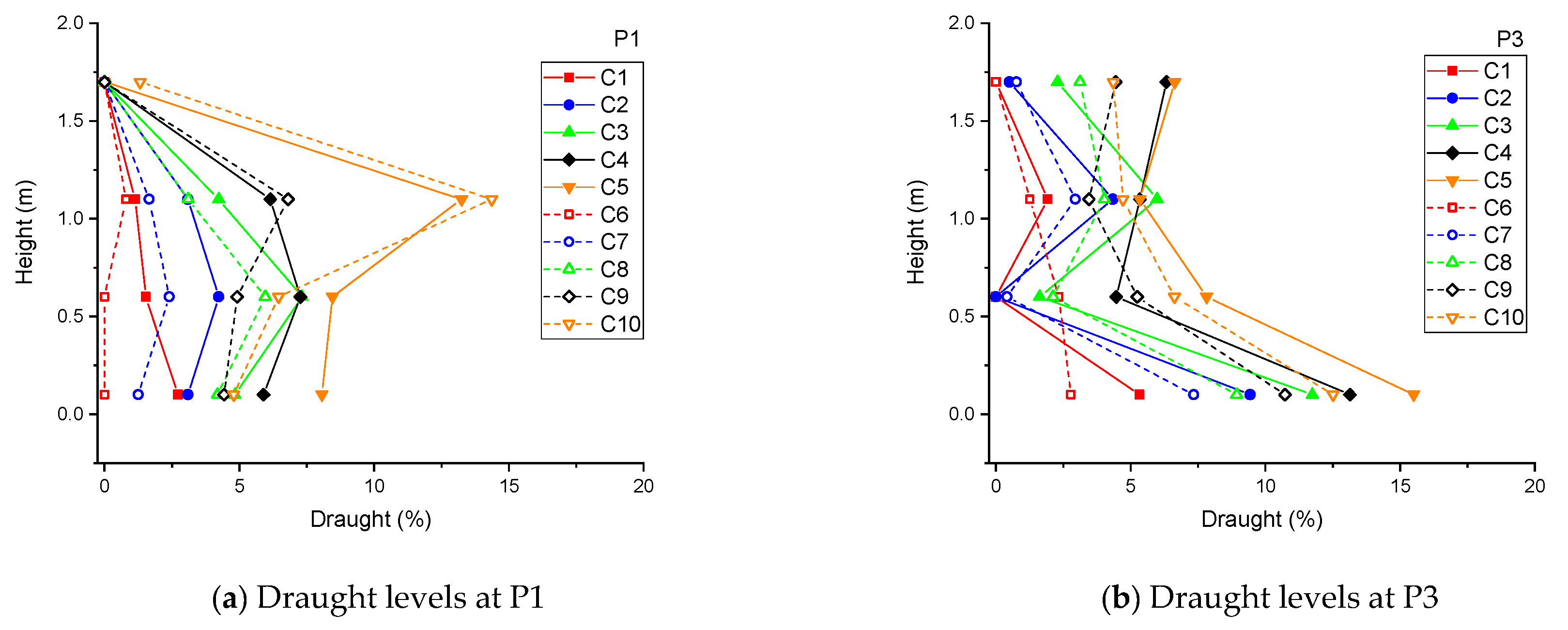
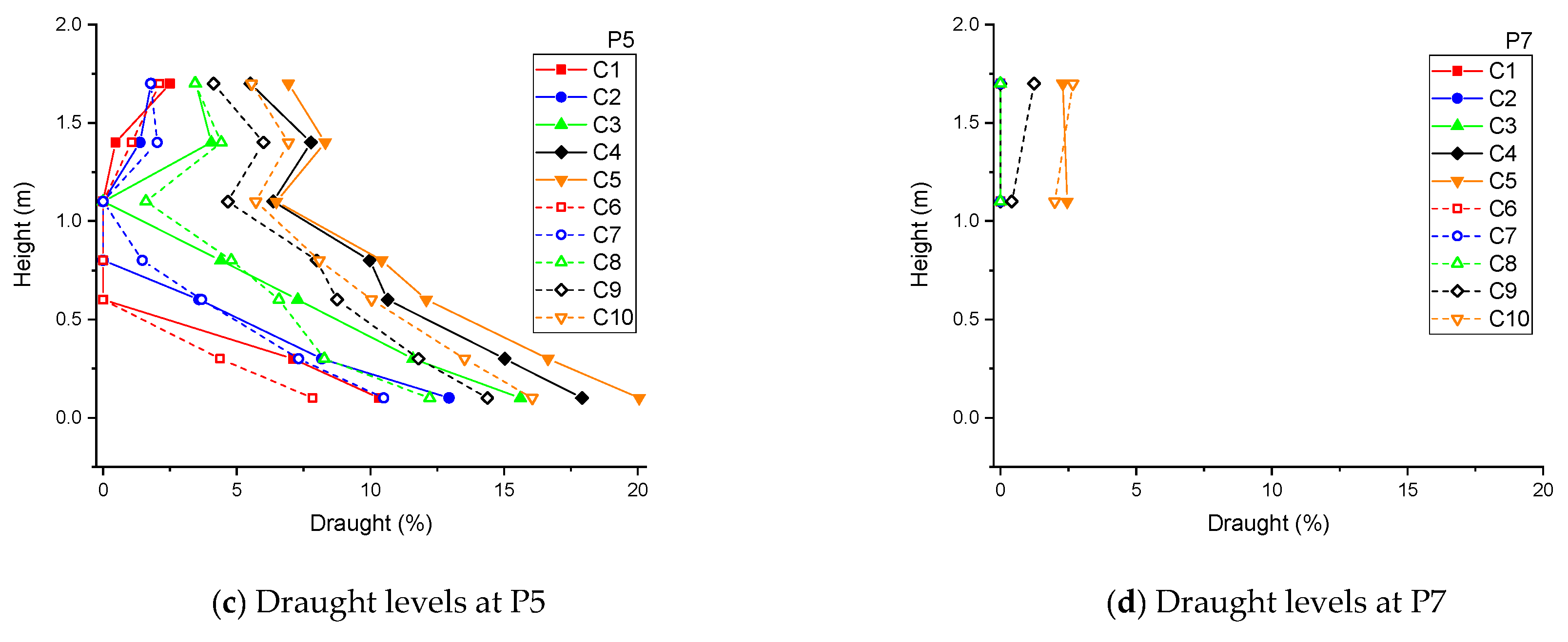
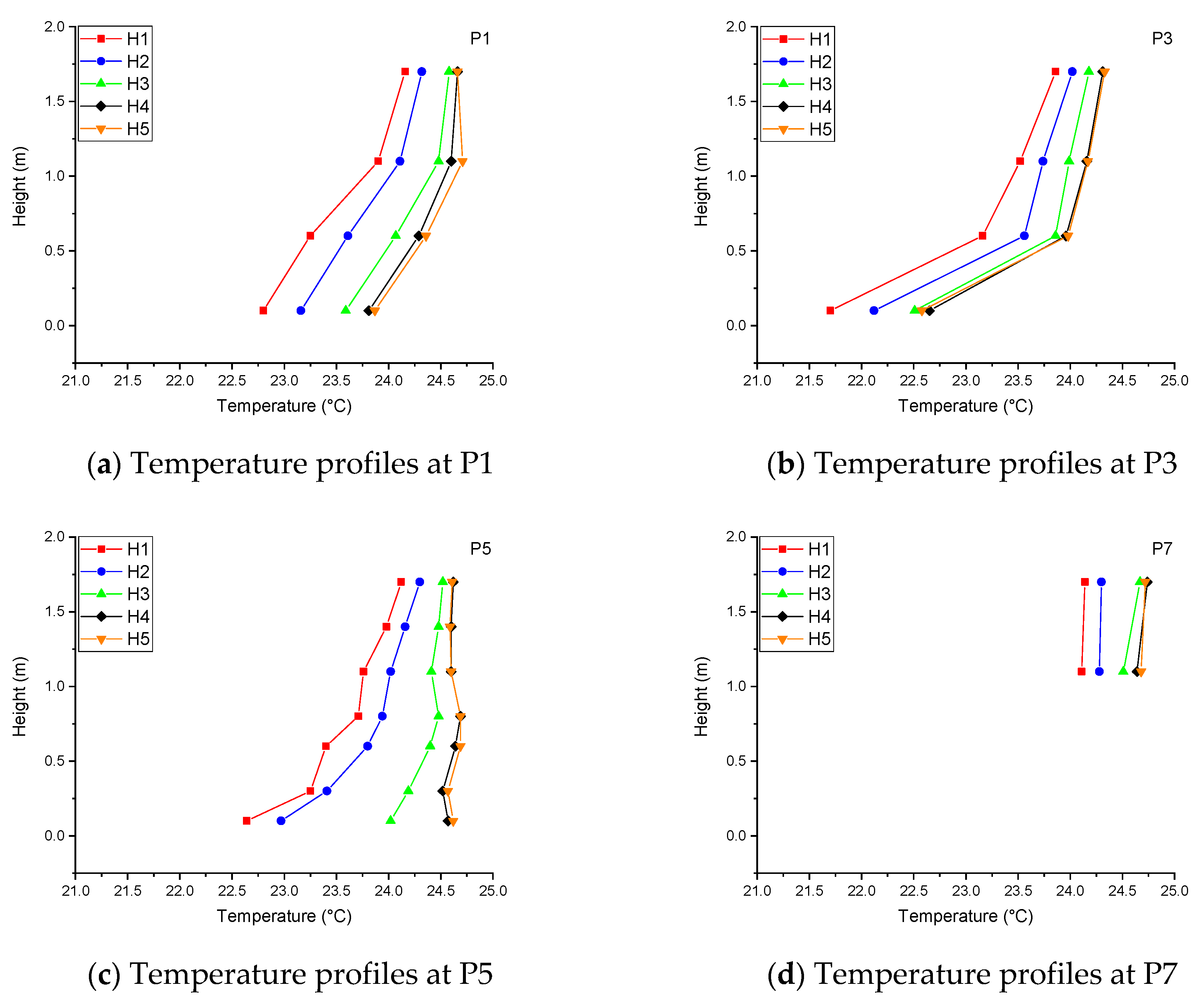
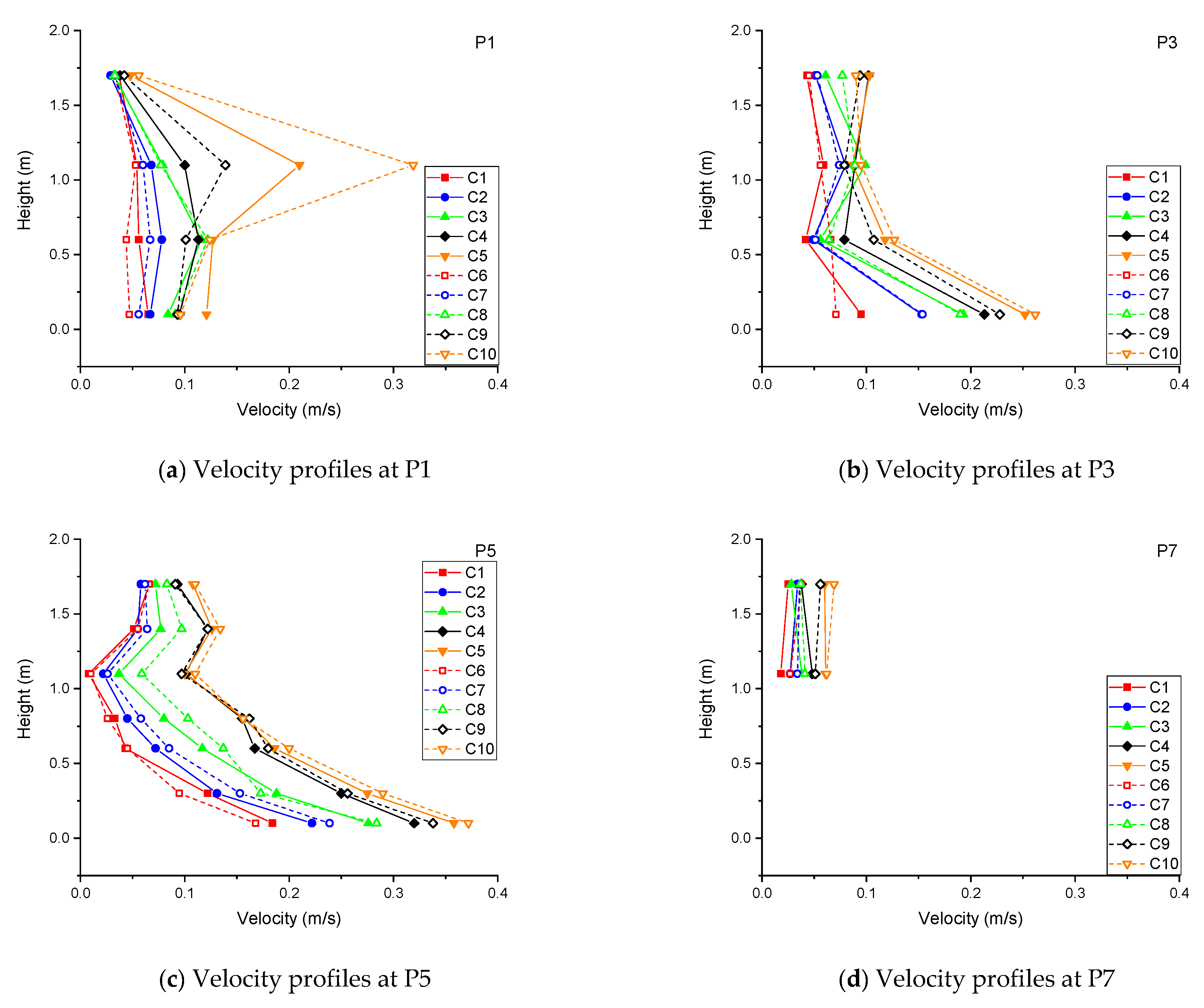
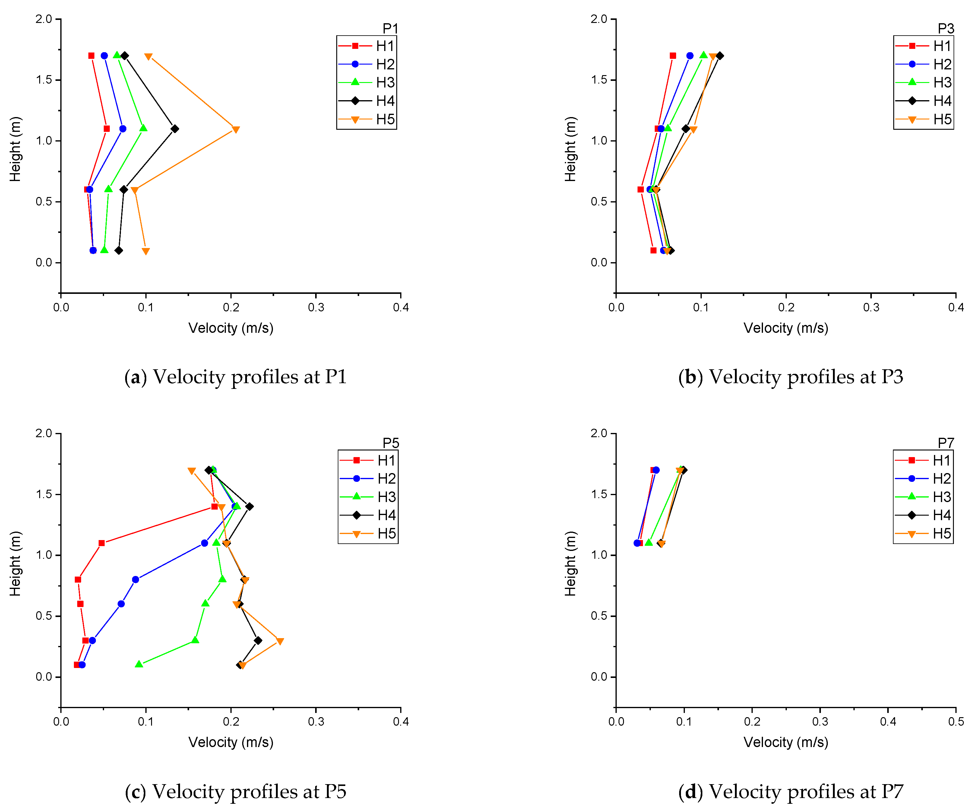
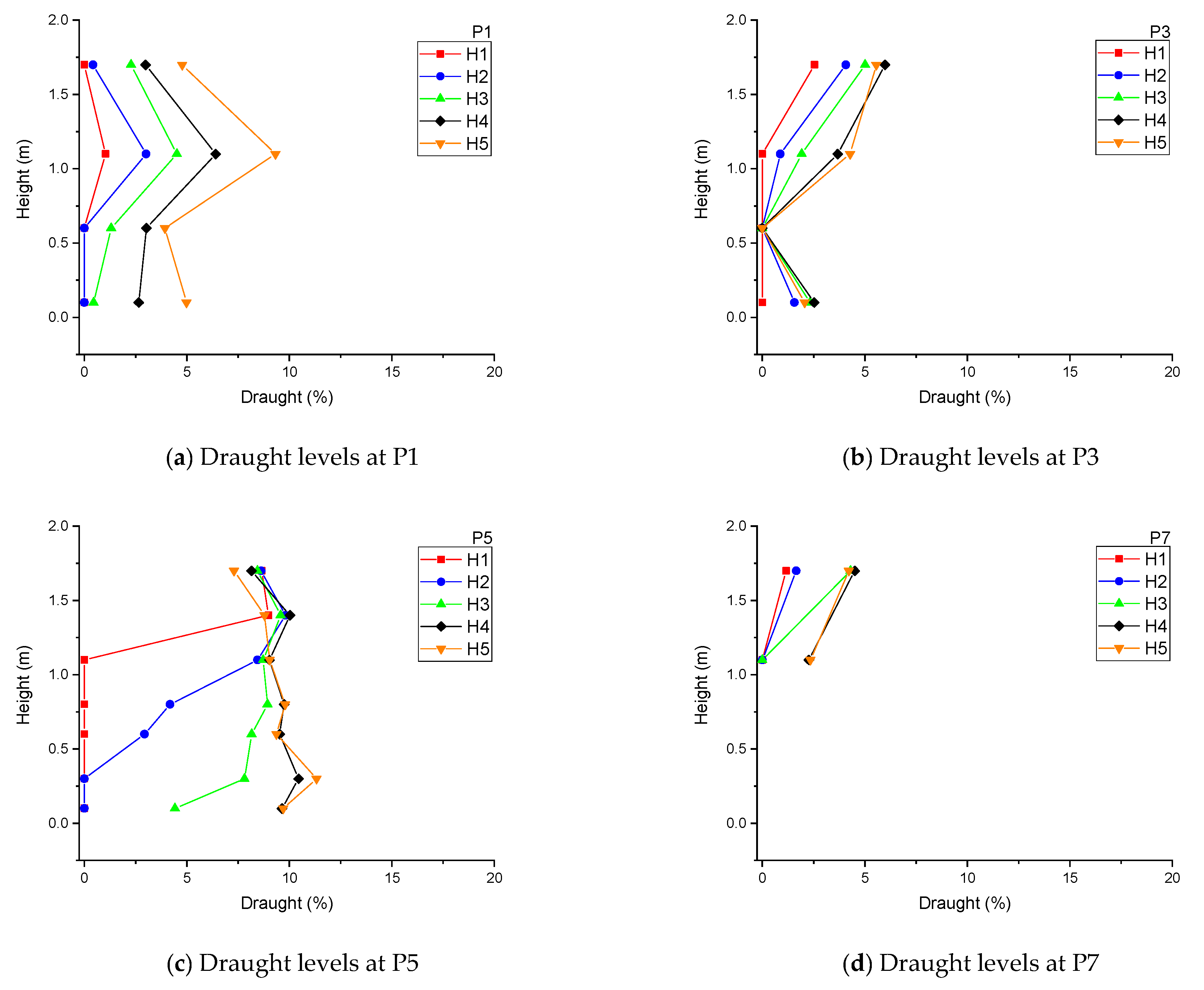
• To carry out measurements of the air velocity and temperature in the office room in order to determine the thermal comfort conditions.
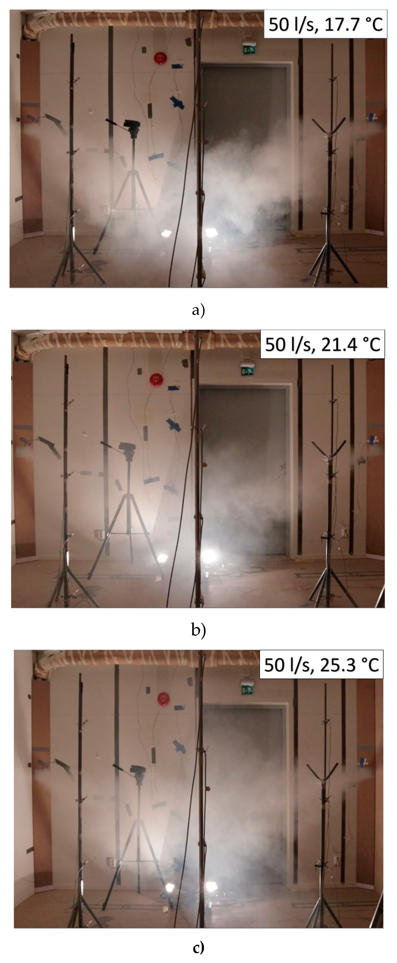
• To conduct flow visualization to ascertain the airflow pattern in the office room.

This study evaluates the suitability of CSV for both cooling and heating applications. Additionally, this research is also a follow-up to two previous studies by Ameen et al. [22,23] in terms of evaluating different air distribution systems when their supply inlets are place in the corners of an office room.

2. Theory and Mathematical Models

This section provides the various key definitions of indoor climate indices which are used in this study. Since this study has a similar methodology and execution as two previous studies [22,23], a more in-depth explanation of these definitions can be found in those articles.

According to ISO 7730 [24], the draught rate (DR) quantifies the discomfort a person experiences due to unwanted cooling of the human body. This index is a function of air velocity, air temperature and turbulent intensity.

Percentage dissatisfied (PD) is related to the local discomfort due to a high vertical air temperature difference between head and ankle. In this study, the temperature difference, ∆T_0.1–1.1 between the ankle level (0.1 m) and the neck level for a seated person (1.1 m) is used. Temperature effectiveness (${\epsilon }_T$) [22,25,26,27] is a parameter that is used to evaluate the effectiveness of heat removal and is defined by

$${\epsilon }_T=\frac{\left(T_o-T_i\right)}{\left({\overline{T}}_{0.1,0.6,1.1}-T_i\right)},$$

(1)

where ${\overline{T}}_{0.1,0.6,1.1}$ is the arithmetic mean air temperature of the heights 0.1, 0.6, and 1.1 m, $T_o$ is the outlet air temperature, and $T_i$ is the supply air temperature. In the case of evaluating how effective space heating is in a location during heating mode [23,28], the following equation can be used

$${\epsilon }_{T\prime }=\frac{\left(T_i-T_o\right)}{\left(T_i-{\overline{T}}_{0.1,0.6,1.1}\right)}.$$

(2)

If ${\epsilon }_{T\prime }$ > 1, this indicates that the temperature in the occupied zone is higher than the outlet. If ${\epsilon }_{T\prime }$ < 1, this indicates that the temperature in the occupied zone is lower than the outlet which means lower utilization of the heat from the ventilation system to the occupied zone. For a perfect mixing ventilation system ${\epsilon }_{T\prime }$ = 1.

The evaluation of ventilation effectiveness can be performed in several ways. Two frequently used indices related to IAQ are air exchange effectiveness (AEE) and air change effectiveness (ACE) [29,30,31].

The inlet Archimedes number (Ar_i) [22,32] is a measure of the relative importance of buoyant and inertia forces. Ar_i is important in building airflows because it combines two important ventilation design parameters, i.e., supply air velocity and room temperature difference. A negative Ar_i value indicates that supply air is flowing downwards towards the floor and a positive value indicates that the it is rising towards the ceiling.

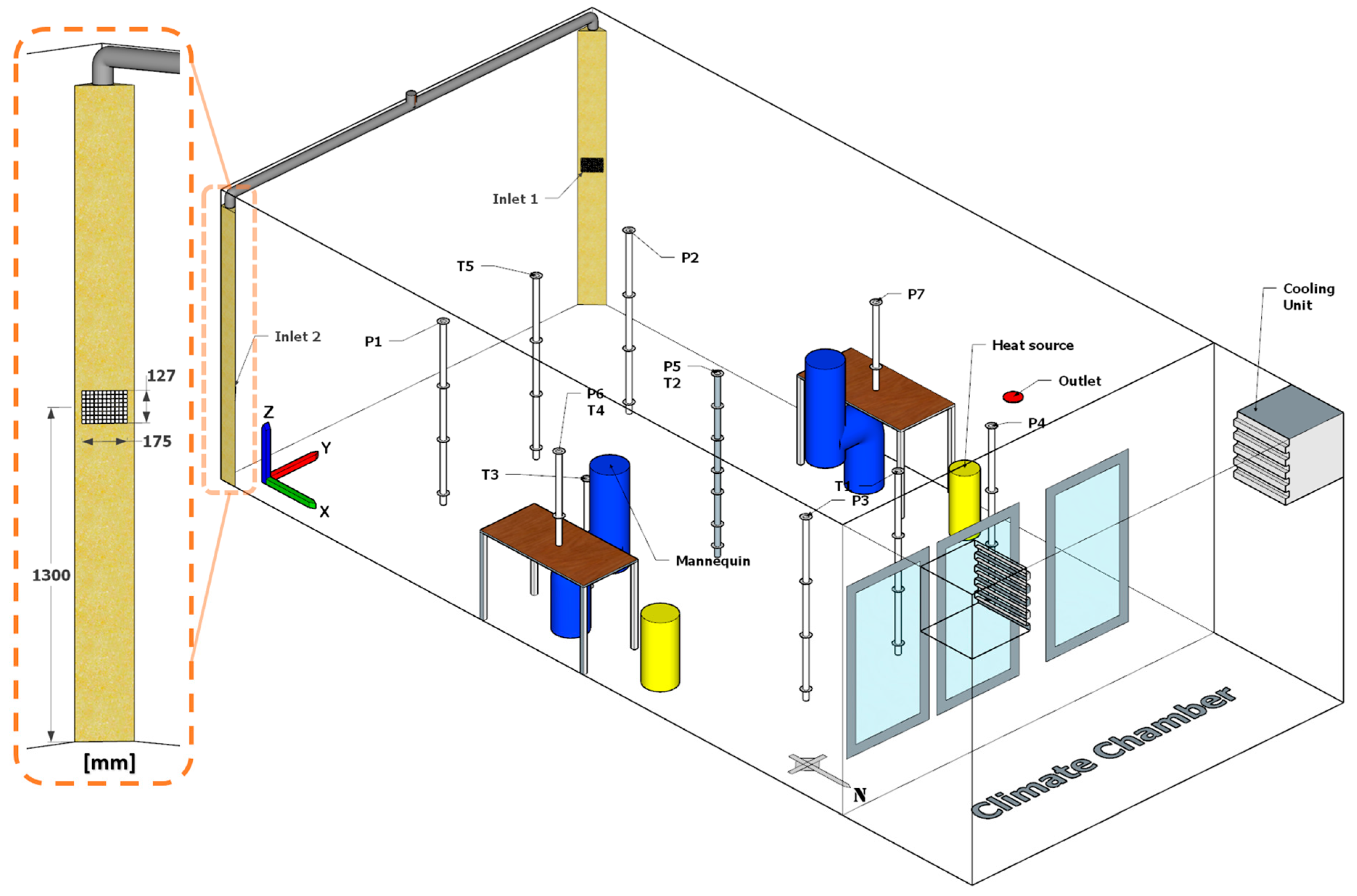
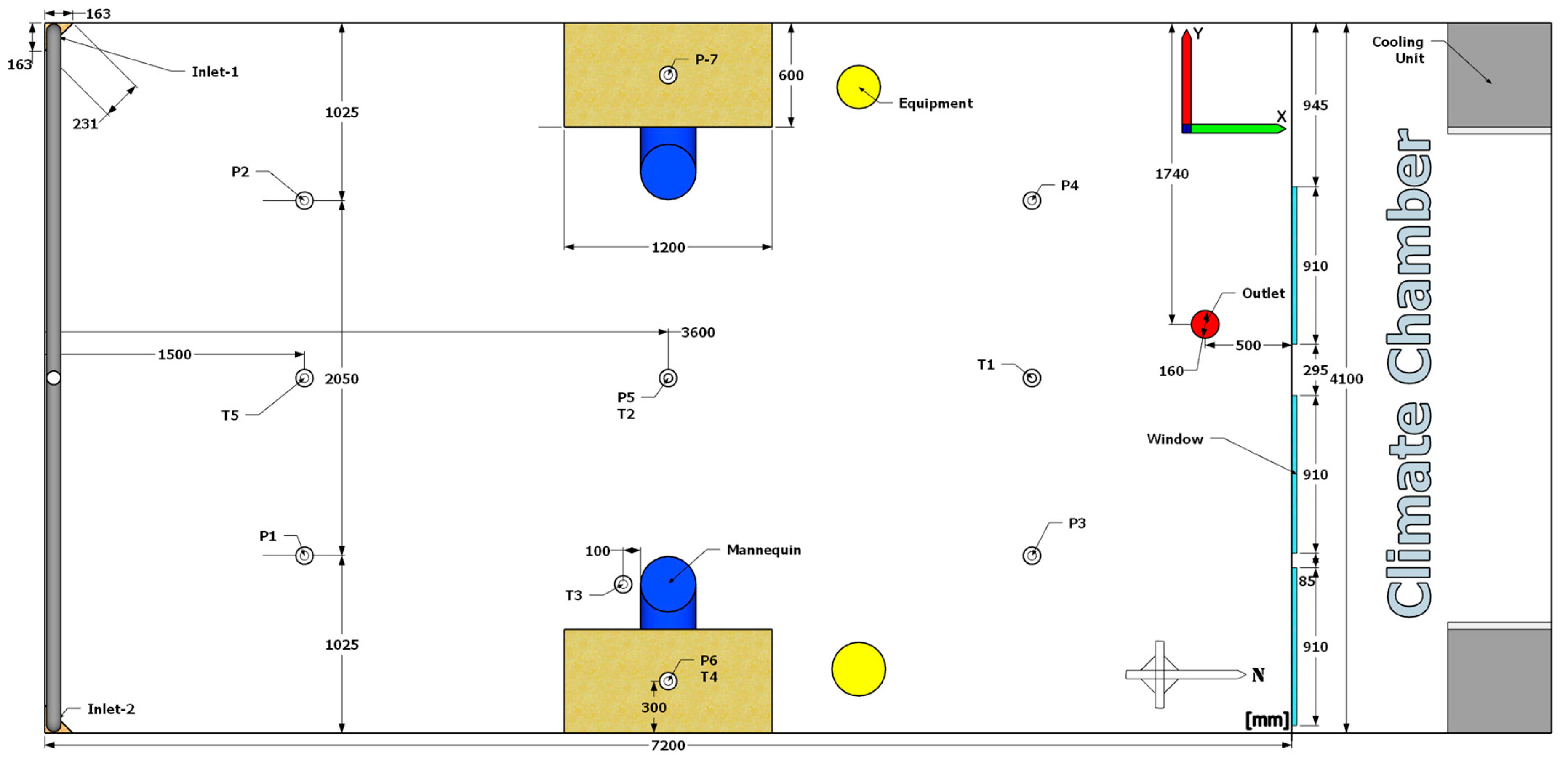
3. Experimental Set-up and Procedure

The study was conducted in one of the test rooms in a laboratory at the University of Gävle. The mock-up office closely resembled the features of the modern office with one exterior wall and three interior walls. The dimensions of the test room were 7.2 m × 4.1m × 2.7 m (L × W × H). The composition of the wall from inside to outside was: 15 mm wood sheet, 35 mm air gap, 15 mm wood sheet, 190 mm insulation, and 5 mm wood sheet. The floor and main ceiling were insulated by a 150 mm thick layer of mineral wool and covered by a layer of plastic sheet to minimize air infiltration. The test room had a suspended ceiling made of 60 cm × 60 cm fiberglass tiles which were hanging 31 cm below the main ceiling. It had three windows located on the northern wall of the test room built in direct connection with a climate chamber. The mock-up office mimicked a shared office with two workstations. The workstations, which were placed about 3.6 m from the air inlet terminals, comprised a table, chair and a seated thermal mannequin each. Each thermal mannequin was made of galvanized tube of 0.32 m diameter covered with fabric to emit the same radiation as an ordinary human being. It had the same area as a human body and produced 100 W. The computer at each workstation was simulated by a 75 W lamp placed inside metallic black cylinder. The total internal heat generated was 350 W. Figure 1 shows the experimental set up of the mock-up office. As a side note, this setup has been evaluated with other types of air distribution systems by the same authors [22,23].

Figure 1 shows the positions of the workstations and the heat sources in relation to the air supply terminals. It also indicates the positions of the measurements for temperature and velocity along with the tracer gas sampling points. The tracer gas sampling points are denoted by letter T along with the position number, e.g., T1, while the points for temperature and velocity measurement are denoted by P such as P1.

The air distribution system had one main inlet which subsequently was divided into two final inlets in the test room. Rectangular straight grill air inlet terminals with dimensions 175 mm × 127 mm each placed at 1.3 m from floor surface to the centreline of the grilles. The effective area of each inlet terminal, excluding the surface area of the grill was 198 cm². The air inlet terminals were placed at the corners of the wall adjoining the south wall. There was only one exhaust terminal located in the ceiling near the northern wall of the room. Figure 1 illustrates the details of the air supply terminals.

Fifteen cases were investigated involving three nominal supply air temperature setpoints: 17.7 °C, 21 °C and 25 °C. At each supply air temperature, five different airflow rates were investigated, i.e., 30, 40, 50, 60 and 70 L/s. The details of the inputs to the different cases are shown in

Table 1. Case conditions for different cases. Case C1–C10 represents cooling cases and H1–H5 represents heating cases.

Case	Supply Flow Rate. (L/s)	Inlet Temp. (°C)	Occupant (W)	Equipment (W)	uin (m/s)	Ari × 10−4
C1	2 × 15	17.7	2 × 100	2 × 75	0.76	484
C2	2 × 20	17.7	2 × 100	2 × 75	1.01	220
C3	2 × 25	17.7	2 × 100	2 × 75	1.26	133
C4	2 × 30	17.7	2 × 100	2 × 75	1.52	80
C5	2 × 35	17.6	2 × 100	2 × 75	1.77	53
C6	2 × 15	21.3	2 × 100	2 × 75	0.76	318
C7	2 × 20	21.2	2 × 100	2 × 75	1.01	181
C8	2 × 25	21.4	2 × 100	2 × 75	1.26	104
C9	2 × 30	21.2	2 × 100	2 × 75	1.52	66
C10	2 × 35	21.2	2 × 100	2 × 75	1.77	40
H1	2 × 15	25.5	2 × 100	2 × 75	0.76	−109
H2	2 × 20	25.4	2 × 100	2 × 75	1.01	−49
H3	2 × 25	25.3	2 × 100	2 × 75	1.26	−24
H4	2 × 30	25.3	2 × 100	2 × 75	1.52	−15
H5	2 × 35	25.4	2 × 100	2 × 75	1.77	−12

. The temperature set points are similar to previous studies made with the same setup [22,23]. Setpoints 17.7 and 21 °C are evaluated through case C1–10 where ‘C’ denotes cooling mode and 25 °C is evaluated through case H1-5 where ‘H’ denotes heating mode.

The concentration decay tracer gas method using SF₆ gas was used in the study. The tracer gas measurements were conducted using the INNOVA 1302 gas monitor and INNOVA 1303 multi-channel sampling unit being augmented by the INNOVA 7260 software installed on the laboratory computer. The INNOVA multi-channel sampling unit has six channels which enabled the measurement of the concentration of the tracer gas at six different positions in the room. The sampling points were strategically selected with one point located in the exhaust. The remaining sampling points were all placed at the breathing zone level, i.e., height of 1.1 m from the floor surface. Positions T1, T2, and T5 were placed in a straight line along the centreline of the room. Position T4 was on the table in front of the thermal mannequin and position T3 was placed on the right-hand side of one thermal mannequin. Position T6 was placed in the exhaust. Due to the limitation of the measuring equipment, no sampling was done near the other mannequin. However, this shortfall has no effect on the results since symmetry of the room was assumed. Before any tracer gas measurements, all the visible air passages were sealed and the room was tested for any leakages—it was found to be acceptably airtight for tracer gas measurements. Figure 2 shows the configuration of the tracer gas sampling points in the test room.

The SF₆ gas was injected into the test room at a concentration of around 350 ppm and the automatic circulating movable fans were operated for the first three minutes to ensure thorough mixing. In order to enhance mixing, the SF₆ gas was injected at multiple points in the room at a height of about 1.8 m. Gas chromatography was used to measure the concentration of the gas in air samples. In each tracer gas test, air samples were collected via a pump connected to the gas chromatography unit. Measurements were performed two times for about four hours each session and the average deviation between the two measurements was less than 2%. The uncertainty of measurements of mean age of air was ± 2.5%. Although, this value can increase when including airflow variation, pressure balancing and air leakage. The uncertainty of ACE in this study was estimated to be in compliance with Appendix E of ASHRAE Standard 129 [29]. The final estimated uncertainty of measured values of ACE was around 7% which was based on the negligible air leakage and the measuring accuracy of the equipment. Other laboratory studies [22,23,33,34] have shown similar results in estimated uncertainty for tracer gas measurements.

The temperature and velocity at selected points were measured using the low-velocity Omni-directional thermistor anemometer type CTA88. The thermistors were connected to a multi-channel logger and were recorded on a personal computer on which LabVIEW program was installed. A total of seven different positions in the room were used for the measurement of the temperature and velocity using the thermistors. For positions represented by points P-1 to P4, measurements were performed at four different heights, i.e., 0.1, 0.6, 1.1 and 1.7 m from the floor surface. For locations P6 and P7, measurements were taken at heights 1.1 and 1.7 m from the floor surface. At point P5, measurements were taken at 0.1, 0.3, 0.6, 0.8, 1.1, 1.4 and 1.7 m from the floor surface. Figure 2 shows the positions in the room at which the air temperature and velocity were measured. All the thermistors were calibrated in a low-velocity calibration unit before use to ensure accurate results. The sampling interval for all measurements was 600 s. The velocity was measured with an accuracy of ± 0.05 m/s excluding directional error with the response time of 0.2 s to 90% of a step change. The uncertainty of temperature measurements was ± 0.2 °C with the response time of 12 s to 90% of value in still air. The surface temperatures for the wall, ceiling, and window were measured using the T-type (copper-constantan) thermocouples connected to an Agilent 34970A data logger and computer. The same type of thermocouples was used to measure the temperature supply air in the main inlet and the two final supply inlets. The calibration of the thermocouples and logger was carried out before and after the measurements to ensure that the accuracy was within the expected range. The climate chamber was maintained at −6.2 ± 0.3 °C during measurement periods for the heating cases. Two cooling units were used to provide an even cooling of the air inside the chamber. The unintended heat losses from the office to the surroundings has been already evaluated in a previous study and has shown to be within acceptable limits [23].

4. Results and Discussion

In this section the flow pattern visualization is presented for 50 L/s. The measured velocity, temperature and draught rate are presented for all positions except for P2, P4 and P6 as the values for these positions are symmetrical to their counterparts, P1, P3 and P7.

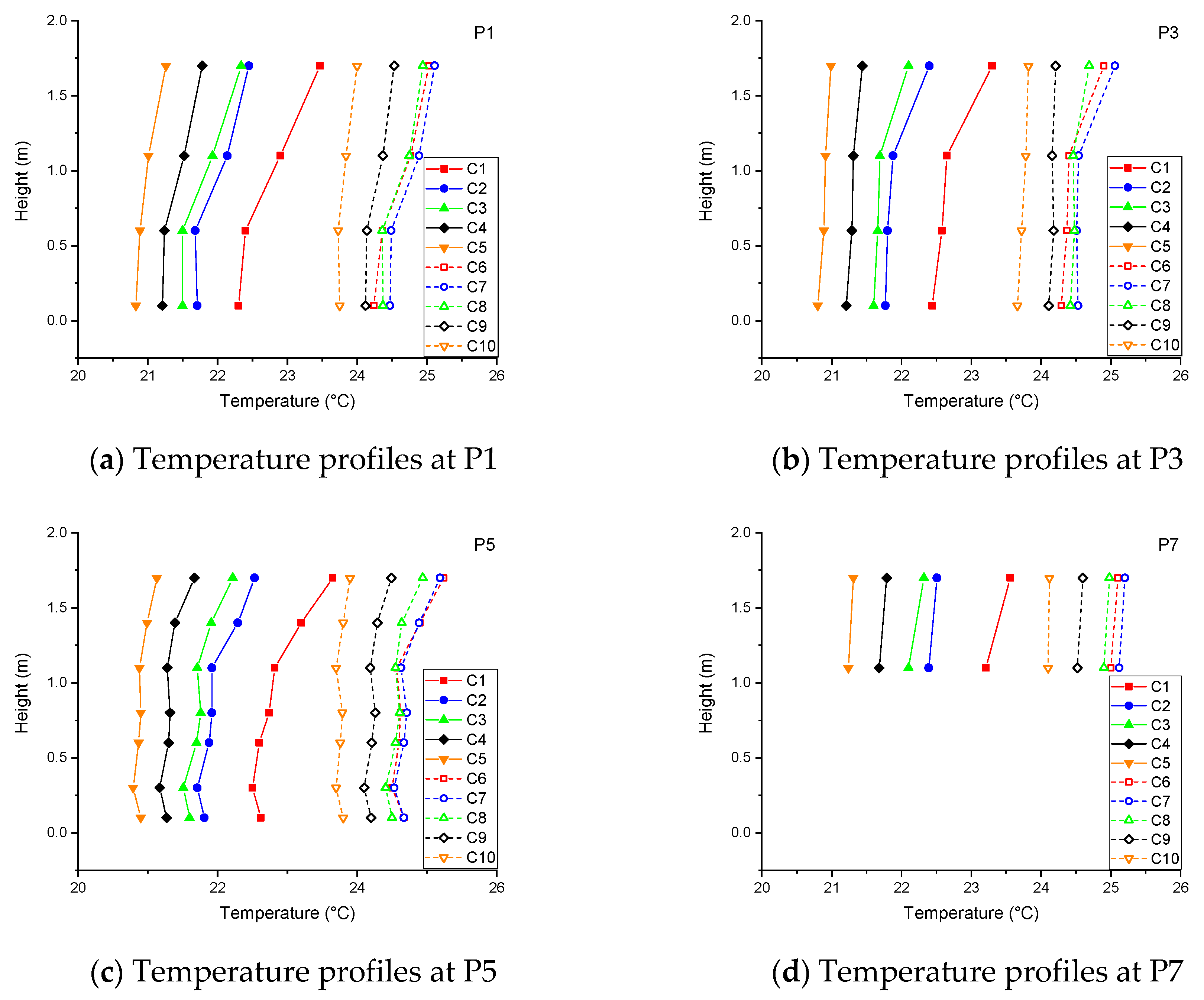
4.1. Flow Pattern and Thermal Conditions

The representative figures for the flow patterns created by the ventilation system at three nominal supply setpoints using the air supply flow rate of 50 L/s are shown in Figure 3. It is clear from Figure 3a, that supplying at 17.7 °C, the airflow quickly tends towards the floor and this tendency decreases with increasing supply temperature. Such behaviour of air inflow has been associated with the SV system in other studies [13]. When supply air temperature was set at 21.4 °C, similar trend was observed as the previous setpoint. For the nominal supply temperature of 25.3 °C, as shown in Figure 3c, at a supply air temperature higher than the room air, much of the supply air remains in the breathing zone and heights above the breathing zone. The created air flow patterns might cause short cut ventilation and stagnation points of the room leading to low ventilation effectiveness [30]. These airflow patterns are also reflected in the Ar_i values presented in Table 1.

Temperatures recorded for positions P1, P3, P5 and P7 for cooling cases are shown in Figure 4. Figure 4a,b show that the vertical temperature profiles in position P1 and P3, looks very similar to one another. C1-5 show overall lower temperatures compared with cases that had higher inlet setpoints, C6-10. Also, C1-5 show a correlation between higher flow rates and lower temperatures. At the breathing level (1.1 m), slightly lower temperatures were recorded compared to 1.7 m level, and this result is similar to that obtained in other studies [12]. Another observation is that there is a very small vertical temperature difference between head and ankle levels, and the existence of lower temperature in the breathing zone level than in the upper levels of the occupied zone in SV system have been reported in other studies [10,13,35,36]. When the nominal supply air temperature was increased to 21 °C, the stratification phenomenon is maintained, but a smaller vertical air temperature difference occurs at 0.5 °C for C6 and about 0.25 °C for C10. At high air flow rates using the nominal supply air temperature of 21 °C, the temperature distribution is similar to a MV system which has nearly uniform temperature distribution [22].

Temperatures recorded for positions P1, P3, P5 and P7 for heating cases are shown in Figure 5. When the nominal supply air temperature was 25 °C, a trend of increasing temperature from the ankle level to the head level was observed. The vertical air temperature difference between the 0.1 m and 1.1 m was highest for the case with lowest air flow rate, i.e., H1 which had 1.25 °C and least with H5 of less than 0.1 °C at P5. P1 which is close to the inlets shows lower stratification than its counterpart on the other side of the room, P3. P3 is affected heavily by the external wall and the cold windows. The cold windows are generating a downdraught flow which is impacting the general airflow in the office room, which is also shown in other studies [23,37,38,39].

In the investigation of the CSV’s ability to provide cooling, the influence of air flow rates was observed; lower temperatures were measured at higher air flow rates. Thus, C5 and C10 showed the lowest temperatures while cases C1 and C6 recorded the highest temperatures in cooling mode as shown in Figure 4 for each temperature setpoint. Relatively larger vertical air temperature difference occurs at lower air flow rates due to lower mixing and this behaviour in SV has been reported in other studies [40]. In assessing the ability of CSV to provide heating in winter climatic conditions, the climate chamber was used. The opposite was observed where the temperature increased with increase in air flow rate with H5 recording highest temperature and H1 the least as indicated in Figure 5. The general trend was that a greater vertical air temperature difference between 0.1 and 1.1 m occurred for the lowest airflow rate at all the nominal supply air temperature setpoints.

Figure 6c illustrates a general trend of decreasing velocity with increase in height under the condition of nominal supply air temperature of 17.7 °C and 21 °C for P5. Highest velocities are recorded at ankle level (0.1 m) and lowest at breathing zone level. This behaviour is attributed to the airflow pattern created in which the relatively cool supply air tends towards the floor while still retaining the high supply momentum. As can be seen in Figure 6c, the values of velocity measured at the breathing zone of a seated sedentary worker in the occupied zone, i.e., at 1.1 m from the ground are all below 0.2 m/s. Lower velocities (less than 0.1 m/s) are measured at the work station above the table which are represented by P7. The velocity conditions in the occupied zone at the breathing zone level all satisfy the design criteria of the maximum mean velocity recommended by ISO 7730 [24].

Position P5 recorded relatively high velocities under all conditions because of its central location and one possible explanation is that the air flow is slightly reinforcement following the coalescing of two air streams from the two air inlet terminals. It worth noting that the results were not perfectly symmetrical for two cases at P1 and P2. Although this should be symmetrical in theory, the authors believe that this is related to maybe some small misalignment of the supply inlets and in combination with a very high flowrate (70 L/s) the main pathway is changed slightly for one of the inlets and it gets closer to the CTA probe on one side compared to the other side. At P5, the velocity measured at 1.4 m is slightly higher than that at 1.1 m. A possible reason for this is that the air circulation created by the nearby thermal plumes.

The velocity measured when the supply air temperature was 25.3 °C are shown in Figure 7. These velocities are heavily affected by the cold downdraught from the windows. In Figure 7c at P5, higher supply air flow rates create a uniform velocity profile whilst the lower flowrates are rising upwards before reaching P5. In addition, the higher flow rates create much more mixing and greater entrainment from the surrounding room air, which results in a very low temperature stratification as seen in Figure 5c.

The draught rate was used to assess the local discomfort due to air movements. Figure 8 shows the draught rate at P1, P3, P5 and P7 for the cooling cases, C1–10. As expected, the draught rate percentage follows the trend of the magnitude of the velocity where it is highest at ankle level and lowest at 1.7 m height for nominal supply air temperature of 17.6 °C. Higher draught rate levels in SV systems have been associated with supply air temperatures below 21 °C [41]. When the nominal supply air temperature was at 17.6 °C, the maximum draught rate was 20% and occurred at ankle level at P5 as shown in Figure 8c. This is due to the high velocity experienced at the position due to amalgamation of the two air streams as mentioned previously.

Increasing the nominal supply air temperature to 21.0 °C showed a slight decrease in draught rate. However, a slight increase is observed at height of 1.4 m. The maximum draught rate which occurs at the ankle level is at 16%. As for the other positions, they follow the same patterns as the velocity profiles.

At the nominal supply air temperature of 25.3 °C for the heating cases, the draught rates all were very low compared to the cooling cases, as seen in Figure 9. The maximum draught rate obtained was about 12% at P5.

The local discomfort due to the vertical temperature difference at P1-P5 in the room was analysed using the PD.

Table 2. Local discomfort (PD) due to high vertical air temperature difference between head and ankle.

Case	PD
	P1	P2	P3	P4	P5
C1	0.5%	0.5%	0.4%	0.4%	0.4%
C2	0.5%	0.4%	0.3%	0.4%	0.3%
C3	0.5%	0.4%	0.3%	0.4%	0.3%
C4	0.4%	0.4%	0.3%	0.4%	0.3%
C5	0.4%	0.3%	0.3%	0.4%	0.3%
C6	0.5%	0.4%	0.3%	0.4%	0.3%
C7	0.4%	0.4%	0.3%	0.4%	0.3%
C8	0.4%	0.4%	0.3%	0.4%	0.3%
C9	0.4%	0.4%	0.3%	0.4%	0.3%
C10	0.3%	0.3%	0.3%	0.3%	0.3%
H1	0.8%	0.8%	1.5%	1.3%	0.8%
H2	0.7%	0.7%	1.2%	0.9%	0.8%
H3	0.7%	0.5%	1.1%	0.8%	0.4%
H4	0.6%	0.5%	1.1%	0.8%	0.3%
H5	0.6%	0.5%	1.2%	0.8%	0.3%

shows the average PD values for all cases. The general trend of decreasing PD with increase in air flow rates is observed in all the cases. As can be seen from the results, all cases conform to requirements of Category A of ISO 7730 on thermal environments [24].

4.2. Ventilation Effectivesness

The temperature effectiveness ${\epsilon }_T$ was used to assess the heat removal capacity of CSV.

Table 3. Average ${\epsilon }_T$ in locations P1–P7 for all cases.

Case	${\mathit{\epsilon }}_{\mathit{T}}$1					${\mathit{\epsilon }}_{\mathit{T}}$2
	P1	P2	P3	P4	P5	P7
C1	1.21	1.23	1.20	1.21	1.17	1.06
C2	1.19	1.20	1.20	1.21	1.18	1.05
C3	1.18	1.17	1.18	1.19	1.17	1.06
C4	1.14	1.13	1.16	1.17	1.15	1.04
C5	1.00	0.99	1.02	1.03	1.01	0.91
C6	1.25	1.27	1.29	1.28	1.19	1.06
C7	1.21	1.23	1.24	1.24	1.19	1.05
C8	1.19	1.17	1.20	1.21	1.17	1.05
C9	1.05	1.05	1.07	1.08	1.05	0.95
C10	0.98	0.98	1.00	1.02	0.99	0.87

¹ calculated by using the arithmetic mean air temperature of the heights 0.1, 0.6, and 1.1 m. ² calculated by using the arithmetic mean air temperature of the height 1.1 m only.

shows the average values of the heat removal effectiveness for all the cooling cases investigated, C1–10.

Table 3 shows that the heat removal effectiveness decreases with increase in air flow rates generally for all cases. At supply air temperature of 17.6 °C, higher efficiencies are recorded for lower air flow rates represented by cases C1 and C2 which closely match the result obtained by other laboratory studies [22]. This result suggests that lower air flow rates can be used to provide cooling and is in line with some features of stratum ventilated spaces reported by some researchers [19,35].

There is a slight increase in the heat removal effectiveness for cases C6 to C8 and decrease for the remaining cases when the nominal supply temperature is increased to 21 °C. This result indicates the potential of energy saving that can be achieved by supplying air at low flow rates at relatively higher temperature. The heat removal effectiveness obtained in cases C1, C2, C6 and C7 shown in Table 3 are very close to those reported for the corner displacement and corner impinging jet ventilations systems [22]. In cooling mode, cases C1 and C6 provided the best heat removal effectiveness for each respective setpoints.

The assessment of CSV to provide heating is shown in

Table 4. Average ${{\epsilon }_T}^{\prime }$ in locations P1–P6 and P7 for all cases.

Case	${{\mathit{\epsilon }}_{\mathit{T}}}^{\prime }$1					${{\mathit{\epsilon }}_{\mathit{T}}}^{\prime }$2
	P1	P2	P3	P4	P5	P7
H1	0.63	0.64	0.51	0.56	0.62	1.00
H2	0.70	0.69	0.55	0.61	0.69	1.12
H3	0.75	0.74	0.51	0.57	0.91	1.17
H4	0.80	0.85	0.51	0.57	1.20	1.26
H5	0.83	0.87	0.50	0.56	1.18	1.25

¹ calculated by using the arithmetic mean air temperature of the heights 0.1, 0.6, and 1.1 m. ² calculated by using the arithmetic mean air temperature of the height 1.1 m only.

. The table shows a general trend of increasing effectiveness of heating the space with increasing air flow rates. However, all points in the room except position P7 which represent the workstation have the temperature effectiveness less than 1. This indicates underutilization of the ventilation system. This result is lower than the ventilation effectiveness obtained for both mixing and stratum ventilation systems in other studies [36]. This assessment is strengthened by the results of the air exchange efficiency shown in

Table 5. Air change effectiveness (ACE), local and average, and air exchange effectiveness (AEE).

Case	ACEp					ACEavg 2	AEE
	T1	T2	T3 1	T4	T5
C1	1.12	1.08	1.06	1.15	1.05	1.09	0.51
C2	1.08	1.06	1.09	1.08	1.08	1.08	0.52
C3	1.08	1.07	1.06	1.06	1.10	1.07	0.53
C4	1.00	1.01	1.01	1.00	1.06	1.02	0.50
C5	1.00	1.02	1.03	1.00	1.12	1.03	0.50
C6	0.99	1.05	1.05	1.04	1.12	1.05	0.47
C7	1.00	1.02	1.00	1.01	1.03	1.01	0.45
C8	1.03	1.05	1.05	1.04	1.07	1.05	0.43
C9	1.06	1.05	1.06	1.06	1.09	1.06	0.48
C10	1.07	1.05	1.08	1.10	1.07	1.07	0.49
H1	1.01	1.03	0.94	0.97	1.10	1.01	0.50
H2	0.99	1.03	0.95	0.98	1.06	1.00	0.44
H3	0.99	1.05	0.95	0.98	1.07	1.01	0.42
H4	0.98	1.05	1.01	1.00	1.09	1.03	0.40
H5	0.99	1.06	1.04	1.00	1.12	1.04	0.49

¹ The location was in the occupied zone close to the mannequin, as also shown in Figure 2. ² ACE_avg is the average ACE value for the measuring points T1–T5.

which are predominantly below 50%. This indicates that the CSV in heating mode performed less than a MV system.

To evaluate the overall ventilation effectiveness at individual positions and for the whole room, ACE_p, ACE_avg, and AEE were used. The results of these indices are presented in Table 5. Under the nominal supply air temperature of 17.6 °C, all the positions show the ACE_avg slightly greater than 1. Slightly higher ACE_avg indices are obtained for low air flow rates, from C1 to C3. This trend illustrates that CSV configuration performs better at lower flow rates. The air exchange efficiency for the mixing ventilation system is 50 %, for displacement system between 50% and 100%, hence the system at this supply air temperature system had the features of MV system. When the supply air temperature was increased to 21.0 °C, similar values for the local air change index were obtained as those at 17.6 °C. However, lower values for the AEE were obtained, slightly below 50%. This gave an indication of some unwanted ventilation occurrences like short-cut ventilation and possibly existence of stagnation zones within the room. The relatively high supply temperature created a flow pattern where some portion of the supplied air did not pass through the lower parts of the room but flowed direct to the higher parts of the room. In this study, only the supply air temperature was increased without any corresponding increase in the room air temperature.

Under the supply air temperature of 25.3 °C, most positions in the room indicated ACE_avg around 1. This indicates a that the performance of the system was around that of a MV system.

From previous studies by other researchers, the ventilation effectiveness of the SV system obtained was between 1.42 and 1.5 [12]. For design purposes the ventilation effectiveness of 1.4 is recommended [13]. The highest local ACE and AEE values obtained for the system were 1.15 and 53%, respectively. These results correlated with low air flow rates i.e., from 30 L/s to 50 L/s. SV system has been associated with better performance at low supply flow rates [36]. The results obtained closely relate to those obtained for the corner mixing ventilation system in previous laboratory study for the cooling mode [22]. This can be attributed to the location of the air inlet devices which were in the corners and far from the occupants; the air reached the occupants after mixing with the room air. The location of the air inlet terminals relative to the occupants has been seen to have significant effect on the mean age of air and contaminant removal performance of the SV system [15]. For better performance of the SV system regarding ACE, a short distance between the occupant and the air supply terminal is desirable [42].

5. Conclusions

The effects of the supply air temperature and supply air flow rates on the performance of the corner stratum ventilation system in a medium sized office was studied. The results show that corner-placed stratum ventilation behaves very similar to a mixing ventilation system when considering air change effectiveness. The performance of the system was better at lower supply air flow rates for heat removal effectiveness and generally higher than that of a typical MV system. For the heating cases, the draught rates were all very low with the maximum measured value of 12%. However, for the cooling cases the maximum draught rate was 20% and occurred at ankle level in the middle of the room. The system satisfied the requirements of the Category A of ISO7730 on thermal environments in terms of PD at all supply air temperature and air flow rate setpoints. A higher temperature gradient was observed for heights greater than 1.1 m and was much pronounced at lower air flow rates for all the nominal supply air temperature setpoints.

References

1. Mazzeo, N. Chemistry, Emission Control, Radioactive Pollution and Indoor Air Quality; InTech: Rijeka, Croatia, 2011; ISBN 978-953-307-316-3. [Google Scholar]
2. Awbi, H.B. Ventilation of Buildings; Routledge: London, UK, 2002; ISBN 1135817413. [Google Scholar]
3. Bakó-Biró, Z.; Clements-Croome, D.J.; Kochhar, N.; Awbi, H.B.; Williams, M.J. Ventilation rates in schools and pupils’ performance. Build. Environ. 2012, 48, 215–223. [Google Scholar] [CrossRef]
4. Nazaroff, W.W. Indoor Particle Dynamics; Indoor Air: Berkeley, CA, USA, 2004; Volume 14, pp. 175–183. [Google Scholar] [CrossRef]
5. IEA World Energy Balances 2018: Overview. 2018, p. 24. Available online: https://webstore.iea.org/world-energy-balances-2018-overview (accessed on 12 October 2018).
6. Cao, G.; Awbi, H.; Yao, R.; Fan, Y.; Sirén, K.; Kosonen, R.; Zhang, J.J. A review of the performance of different ventilation and airflow distribution systems in buildings. Build. Environ. 2014, 73, 171–186. [Google Scholar] [CrossRef]
7. Fong, M.; Lin, Z.; Fong, K.; Hanby, V.; Greenough, R. Life cycle assessment for three ventilation methods. Build. Environ. 2017, 116, 73–88. [Google Scholar] [CrossRef]
8. Rim, D.; Novoselac, A. Ventilation effectiveness as an indicator of occupant exposure to particles from indoor sources. Build. Environ. 2010, 45, 1214–1224. [Google Scholar] [CrossRef]
9. Lin, Z.; Chow, T.T.; Tsang, C.; Fong, K.; Chan, L. Stratum ventilation—A potential solution to elevated indoor temperatures. Build. Environ. 2009, 44, 2256–2269. [Google Scholar] [CrossRef]
10. Lin, Z.; Chow, T.; Tsang, C. Stratum ventilation? A conceptual introduction. In Proceedings of the 10th International Conference on Indoor Air Quality and Climate (Indoor Air 2005), Beijing, China, 4–9 September 2005; pp. 3260–3264. [Google Scholar]
11. Tian, L.; Lin, Z.; Liu, J.; Yao, T.; Wang, Q. The impact of temperature on mean local air age and thermal comfort in a stratum ventilated office. Build. Environ. 2011, 46, 501–510. [Google Scholar] [CrossRef]
12. Tian, L.; Lin, Z.; Wang, Q. Experimental investigation of thermal and ventilation performances of stratum ventilation. Build. Environ. 2011, 46, 1309–1320. [Google Scholar] [CrossRef]
13. Lin, Z.; Yao, T.; Chow, T.T.; Fong, K.; Chan, L. Performance evaluation and design guidelines for stratum ventilation. Build. Environ. 2011, 46, 2267–2279. [Google Scholar] [CrossRef]
14. Cheng, Y.; Lin, Z. Experimental study of airflow characteristics of stratum ventilation in a multi-occupant room with comparison to mixing ventilation and displacement ventilation. Indoor Air 2015, 25, 662–671. [Google Scholar] [CrossRef]
15. Lin, Z.; Chow, T.; Tsang, C. Validation of a CFD model for research into stratum ventilation. Int. J. Vent. 2006, 5, 345–363. [Google Scholar] [CrossRef]
16. Wang, X.; Lin, Z. An experimental investigation into the pull-down performances with different air distributions. Appl. Therm. Eng. 2015, 91, 151–162. [Google Scholar] [CrossRef]
17. Shao, X.; Wang, K.; Li, X.; Lin, Z. Potential of stratum ventilation to satisfy differentiated comfort requirements in multi-occupied zones. Build. Environ. 2018, 143, 329–338. [Google Scholar] [CrossRef]
18. Lin, Z.; Lee, C.K.; Fong, S.; Chow, T.T.; Yao, T.; Chan, A. Comparison of annual energy performances with different ventilation methods for cooling. Energy Build. 2011, 43, 130–136. [Google Scholar] [CrossRef]
19. Fong, M.; Lin, Z.; Fong, K.; Chow, T.T.; Yao, T. Evaluation of thermal comfort conditions in a classroom with three ventilation methods. Indoor Air 2011, 21, 231–239. [Google Scholar] [CrossRef] [PubMed]
20. Ruparathna, R.; Hewage, K.; Sadiq, R. Improving the energy efficiency of the existing building stock: A critical review of commercial and institutional buildings. Renew. Sustain. Energy Rev. 2016, 53, 1032–1045. [Google Scholar] [CrossRef]
21. Tian, L.; Lin, Z.; Liu, J.; Wang, Q. Numerical study of indoor air quality and thermal comfort under stratum ventilation. Prog. Comput. Fluid Dynamic 2008, 8, 541–548. [Google Scholar] [CrossRef]
22. Ameen, A.; Cehlin, M.; Larsson, U.; Karimipanah, T. Experimental investigation of ventilation performance of different air distribution systems in an office environment -cooling mode. Energies 2019, 12, 1354. [Google Scholar] [CrossRef]
23. Ameen, A.; Cehlin, M.; Larsson, U.; Karimipanah, T. Experimental investigation of ventilation performance of different air distribution systems in an office environment-heating mode. Energies 2019, 12, 1835. [Google Scholar] [CrossRef]
24. ISO 7730. Ergonomics of the Thermal Environment-Analytical Determination and Interpretation of Thermal Comfort Using Calculation of the PMV and PPD Indices and Local Thermal Comfort Criteria; ISO: Geneva, Switzerland, 2005.
25. Qingyan, C.; Van Der Kooi, J.; Meyers, A. Measurements and computations of ventilation efficiency and temperature efficiency in a ventilated room. Energy Build. 1988, 12, 85–99. [Google Scholar] [CrossRef]
26. Artmann, N.; Jensen, R.L.; Manz, H.; Heiselberg, P. Experimental investigation of heat transfer during night-time ventilation. Energy Build. 2010, 42, 366–374. [Google Scholar] [CrossRef]
27. Olesen, B.W.; Simone, A.; KrajcÍik, M.; Causone, F.; Carli, M.D. Experimental study of air distribution and ventilation effectiveness in a room with a combination of different mechanical ventilation and heating/cooling systems. Int. J. Vent. 2011, 9, 371–383. [Google Scholar] [CrossRef]
28. Rabani, M.; Madessa, H.B.; Nord, N.; Schild, P.; Mysen, M. Performance assessment of all-air heating in an office cubicle equipped with an active supply diffuser in a cold climate. Build. Environ. 2019. [Google Scholar] [CrossRef]
29. ASHRAE Standard 129-1997 (RA 2002). Measuring Air Change Effectiveness; ASHRAE: Atlanta, GA, USA, 2002.
30. Mundt, M.; Mathisen, H.M.; Moser, M.; Nielsen, P.V. Ventilation Effectiveness; REHVA: Brussels, Belgium, 2004; ISBN 978-29-6004-680-9. [Google Scholar]
31. Breum, N. Ventilation efficiency in an occupied office with displacement ventilation-a laboratory study. Environ. Int. 1992, 18, 353–361. [Google Scholar] [CrossRef]
32. Both, B.; Szánthó, Z. Objective investigation of discomfort due to draught in a tangential air distribution system: Influence of air diffuser’s offset ratio. Indoor Built Environ. 2018, 27, 1105–1118. [Google Scholar] [CrossRef]
33. Buratti, C.; Mariani, R.; Moretti, E. Mean age of air in a naturally ventilated office: Experimental data and simulations. Energy Build. 2011, 43, 2021–2027. [Google Scholar] [CrossRef]
34. Cehlin, M.; Karimipanah, T.; Larsson, U.; Ameen, A. Comparing thermal comfort and air quality performance of two active chilled beam systems in an open-plan office. J. Build. Eng. 2019, 22, 56–65. [Google Scholar] [CrossRef]
35. Lin, Z.; Chow, T.; Tsang, C.; Chan, L.; Fong, K. Effect of air supply temperature on the performance of displacement ventilation (Part I)-thermal comfort. Indoor Built Environ. 2005, 14, 103–115. [Google Scholar] [CrossRef]
36. Kong, X.; Xi, C.; Li, H.; Lin, Z. A comparative experimental study on the performance of mixing ventilation and stratum ventilation for space heating. Build. Environ. 2019, 157, 34–46. [Google Scholar] [CrossRef]
37. Ge, H.; Fazio, P. Experimental investigation of cold draft induced by two different types of glazing panels in metal curtain walls. Build. Environ. 2004, 39, 115–125. [Google Scholar] [CrossRef]
38. Manz, H.; Frank, T. Analysis of thermal comfort near cold vertical surfaces by means of computational fluid dynamics. Indoor Built Environ. 2004, 13, 233–242. [Google Scholar] [CrossRef]
39. Jurelionis, A.; Isevičius, E. CFD predictions of indoor air movement induced by cold window surfaces. J. Civ. Eng. Manag. 2008, 14, 29–38. [Google Scholar] [CrossRef]
40. Yao, T.; Lin, Z. An experimental and numerical study on the effect of air terminal types on the performance of stratum ventilation. Build. Environ. 2014, 82, 431–441. [Google Scholar] [CrossRef]
41. Cheng, Y.; Lin, Z.; Fong, A.M. Effects of temperature and supply airflow rate on thermal comfort in a stratum-ventilated room. Build. Environ. 2015, 92, 269–277. [Google Scholar] [CrossRef]
42. Lee, C.; Fong, K.; Lin, Z.; Chow, T. Year-round energy saving potential of stratum ventilated classrooms with temperature and humidity control. HVAC&R Res. 2013, 19, 986–991. [Google Scholar] [CrossRef]
Figure 1. Isometric layout of the mock-up office test chamber.
Buildings 09 00169 g001
Figure 2. Measurement positions and schematic top-view layout of the office room, including the climate chamber, which is the same layout as in [22].
Buildings 09 00169 g002
Figure 3. Flow visualization: (a) air flow patterns at 50 L/s and 17.7 °C, (b) air flow patterns at 50 L/s and 21.4 °C, (c) air flow patterns at 50 L/s and 25.3 °C.
Buildings 09 00169 g003
Figure 4. Air temperature profiles at position P1 (a), P3 (b), P5 (c) and P7 (d) for cooling cases (C1–C10).
Buildings 09 00169 g004
Figure 5. Air temperature profiles at position P1 (a), P3 (b), P5 (c) and P7 (d) for heating cases (H1–H5).
Buildings 09 00169 g005
Figure 6. Velocity profiles at position P1 (a), P3 (b), P5 (c) and P7 (d) for cooling cases (C1–C10).
Buildings 09 00169 g006
Figure 7. Velocity profiles at position P1 (a), P3 (b), P5 (c) and P7 (d) for heating cases (H1–H5).
Buildings 09 00169 g007
Figure 8. Draught levels at position P1 (a), P3 (b), P5 (c) and P7 (d) for cooling cases (C1–C10).
Buildings 09 00169 g008aBuildings 09 00169 g008b
Figure 9. Draught levels at position P1 (a), P3 (b), P5 (c) and P7 (d) for heating cases (H1–H5).
Buildings 09 00169 g009