Abstract
Operations and maintenance optimization are primary issues in Facility Management (FM). Moreover, the increased complexity of the digitized assets leads Facility Managers to the adoption of interdisciplinary metrics that are able to measure the peculiar dynamics of the asset-service system. The aim of this research concerns the development of a cross-domain Decision Support System (DSS) for maintenance optimization. The algorithm underpinning the DSS enables the maintenance optimization through a wiser allocation of economic resources. Therefore, the primary metric encompassed in the DSS is a revised version of the Facility Condition Index (FCI). This metric is combined with an index measuring the service life of the assets, one measuring the preference of the owner and another measuring the criticality of each component in the asset. The four indexes are combined to obtain a Maintenance Priority Index (MPI) that can be employed for maintenance budget allocation. The robustness of the DSS has been tested on an office building in Italy and provided good results. Despite the proposed algorithm could be included in a wider Asset Management system employing other metrics (e.g., financial), a good reliability in the measurement of cross-domain performance of buildings has been observed.
1. Introduction
In Facility Management (FM), performance measurement is one of the primary issues to both ensure a high-quality built environment for owners and users, and to enhance competitiveness of the organization providing FM services. The performance measurement assumes a strategic role for the assessment and monitoring of critical factors within an organization [1], and therefore needs a particular attention in the context of improved decision-making.
Currently the FM context is changing. The physical asset should no longer be characterized only according to its presence and existence in the real estate; it should be conceived as strictly related to data and information which are used for its operation and that are generated through its use [2]. This trend can be named the digitization of the built environment. The digitization, together with the sustainability, is one of the driving forces in FM [3] and can be intended as those dynamics that are currently leading the research in FM and the development of new and more effective business processes in the industry. The digitization is shaping a different approach, which should be considered when dealing with physical assets [4]. The digitized asset is composed of the physical asset integrated with data related to the different phases of its life cycle. This strict integration is due to the contemporary need for collaboration and the interdisciplinary exchange of competences which requires new approaches for working on the digital built environment. Moreover, FM has always been related to the information management tools and took advantage of this strict interrelation from the first Computer Aided Facility Management (CAFM), followed by CAD tools and Integrated Workplace Management Systems (IWMS), up to Computerized Maintenance Management Systems (CMMS) [5].
More recently FM has been more and more strongly integrated within the Building Information Modeling (BIM), due to the wide adoption of this approach in design and construction phases [6]. A primary challenge in this field concerns how to maintain and effectively employ information coming from the previous phases in the use phase of assets, without a loss of reliability, in order to exploit the collaboration and integration capabilities offered by the BIM [7] approach.
Thanks to this dynamic, in FM new services can be delivered through the use of the digitized assets. Typically, FM has been conceived as a discipline composed of a set of theories and practices carried out for the reducing costs and inefficiencies of the non-core business, in order to increase the productivity of the core business of an organization. Today this trend is changing, and the development of FM services is more closely targeted towards the optimization of the core business of the organization [8].
The digitization brings new dynamics, enabled by the availability and accessibility of data, in all the life cycle phases of the assets. One of them concerns the servitization of the built environment. In manufacturing, the servitization is intended as a strategy for the improvement of the competitiveness of organizations [9] through the inclusion of a set of services, within the selling of a product. These services can be activated even after the transaction [10]. In management of the digital built environment, the demand for efficient and integrated spaces is a key enabler for success and competitiveness of the core business. Accordingly, the building is conceived not only as a physical asset but also as an integrated system composed of the physical asset and the services that can be provided to the users through its use [8].
The Aim of the Research
Traditional performance measurement categories (e.g., financial, functional, physical, user satisfaction [11]) are no longer suitable metrics for measurement of cross-domain performances offered by the digitized and servitized assets.
Accordingly, the research question concerns how effectively measure cross-domain performances of digitized assets. Moreover, once these performances have been measured, how is it possible to optimize them, in order to achieve an improved Facilities Management of digitized assets? Therefore, this research aims at proposing a cross-domain Decision Support System (DSS) for the allocation of maintenance budgets. The maintenance cost performance of the asset has been computed through the Facility Condition Index (FCI), one of the most acknowledged indicators measuring the technical performance of the building and its components through an economic metric. This indicator has been combined with a set of further parameters: the D index, measuring the service life of the component; the C index measuring the criticality as the consequence of the failure of the component for the effective execution of the core business of the organization occupying the asset; the P index measuring the preference of the asset owner for the execution of the core business. These indicators are combined together for each building component (asset) and are ranked on a scale from 0 to 1, through the calculation of the Maintenance Priority Index (MPI): the simple average of the four metrics.
Assuming a reduced budget (not enough to cover all maintenance costs), an optimization algorithm has been developed, thus the economic resources can be allocated to those components presenting the highest MPI value.
In order to test the robustness of the proposed methodology, the DSS has been applied to a case study involving an office building in Erba, Italy. A simulation with reduced maintenance budget has been carried out, demonstrating the possibility of effectively driving different maintenance policies, according to a variation of the C and P indexes.
2. State of the Art
In Asset and Facilities Management, performance measurement can be considered as a powerful mean for decision-making [12]. This activity can be seen both as a factor for enhancing the competitiveness of an organization and as a learning process within the organization [13], which allows the continuous improvement in the decision-making process, for the effective delivery of better services [14]. Performance measurement is always tied to the use of specific Key Performance Indicators (KPIs), which allow us to synthetize phenomena, without losing the systemic value of the information [15]. KPIs are obtained through the refinement of raw data, therefore they are employed at different decision-making levels, depending on the management needs. Typically, three decision-making levels can be recognized when dealing with performance measurement: strategic, tactical and operational [16,17].
Performance metrics are often aggregated to support a decision-making process and this aggregation can vary according to the disciplinary field, the type of organization and the decision-making level [18]. One of the most acknowledged methods for assessment of performances within an organization is the Balanced Score Card (BSC) framework: A model for measurement and management of strategic performances within an organization [1]. The balanced score card gave rise to the definition of specialized KPIs for FM [3].
In management of the built environment, metrics are usually domain-specific and related to technical, functional, economic/financial performances [19]. For a definition of effective DSS, metrics are seldom selected among the same domain, to avoid the excessive specialization of the performance assessment [14,20]. However, one of the most acknowledged indicators for measurement of technical performances through an economic dimension is the Facility Condition Index (FCI). This indicator was introduced for the first time by the National Association of College and University Business Officers (NACUBO) and Rush (1991) [21], and it is widely used for making informed decisions in AM and FM [11,22,23].
The Facility Condition Index
The FCI allows us to quantify on a scale from 0 to 100 the condition of the assets. The metric is a ratio between the Deferred Maintenance (DM) and the Current Replacement Value (CRV) of each component of an asset and can be calculated at different scales: from the single component in a building, until the whole building in a portfolio [24]. The basic equation used for the calculation of the metric is (1):
where:
- DM is the cost of the deferred maintenance, defined as the costs of the maintenance operations that should have been done but it had been deferred,
- CRV is the current replacement value of the component or the same asset [25].
The result of the calculation is evaluated on three or four levels, on a scale from 0 to 100%, where 0 is the best value:
- good: 0%–5%,
- fair: 5%–10%,
- poor: 10%–30%,
- critical: 30%–100%.
The FCI, since its first publication, has been adopted for leading maintenance policies of assets portfolios of many departmental organizations in the United States of America (USA) [26]. Among them, the Department of the Interior (DoI) has published a set of documents and guidelines which contributed in the standardization of procedures and workflows related to the calculation of the metric [26,27,28]. However, a standardized calculation methodology has not been defined yet.
In literature, other definitions of the indicator can be found. These versions can be considered as improved variations of the original formula. Despite being a powerful mean for the calculation of the technical performances of the assets, this metric needs to be carefully calculated and often when combined with further indicators, is able to describe other performances not directly related to the technical and economic performance of the assets. More in general, recent versions of the indicator show differences in terms calculation of the DM and CRV. Some versions, for instance, consider the effect of obsolescence due to lack of compliance with codes in the calculation [29]. In some other cases, the DM is computed considering even the renewals and improvements [24]. Other approaches for the calculation of the DM are specific for the evaluation of historical assets [25]. Therefore, the USA governmental guidelines [25,30] suggest employing a combined version of the FCI for being more effective in the computation of the overall maintenance performance. This enhanced version encompasses in the calculation also major rehabilitation, replacement and maintenance recommendations registered during the periodic Condition Assessment (CA). These factors are used for the calculation of a composed index: the FCIcomp (2):
where:
- DM is the deferred maintenance as defined for Equation (1),
- DMmr is the cost of major rehabilitations and replacements,
- DMim is the cost of the maintenance and repair recommendations highlighted during the periodic CA.
Finally, the FCIcomp is used for the calculation of a Condition Index (CIcomp) (3):
The CIcomp can be considered as one of the examples of how the FCI is modified in order to describe a wider array of phenomena. Other application of the FCI can be found in literature, the most of them stemming from the need for a more comprehensive performance measurement tools that are able to catch the complexity of the physical asset, while measuring performances belonging to different disciplinary fields [23,31]. A good example of how the FCI could be associated with other metrics involves coupling with the Asset Priority Index (API) [32]: a metric which measures the relevance of the asset according to the objective that the owning organization wants to achieve through its use. The API have been employed by many private and public organizations [33,34], being a powerful qualitative indicator that is able to correct the FCI according to the strategic importance of an asset, provided by the managing or owning organization.
In summary, the FCI can be considered as a powerful aggregated metric for the measurement of the maintenance performance of the assets, through an economic dimension. Nevertheless, some drawbacks can be highlighted. The most evident concerns its feature of being driven by the dimension of the denominator: Two components presenting the same DM but different CRV are ranked differently, since the ratio would penalize the component with the highest CRV. This issue does not allow us to use the FCI itself for prioritization of maintenance interventions, since the metric will always tend to penalize components with small CRV. A second drawback involves the evident technical nature of the indicator, not considering other phenomena but only the maintenance performance. Therefore, the FCI provides valuable information of the technical performance, despite needing to be associated with other metrics to be considered an effective tool for decision-making. Through this research these main two issues are addressed and a flexible and cross-domain DSS is proposed.
3. Materials and Methods
In this article a DSS for the optimization of maintenance budget is presented. The maintenance budget is allocated thanks to the inclusion of the FCI in the DSS to obtain the Maintenance Priority Index (MPI), thanks to the combination with 3 KPIs measuring the age of the assets (D), their criticality (C) and the preference of the owner (P). The three metrics are described in detail in the following paragraphs. Figure 1 represents the process developed for the calculation of the algorithm.
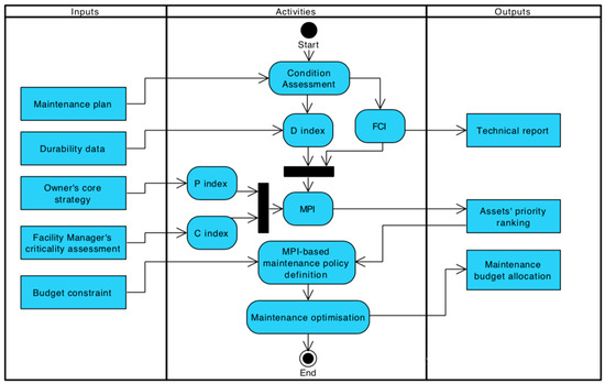
Figure 1.
Process adopted for the development of the algorithm underpinning the Decision Support System (DSS).
The four KPIs were aggregated in a final equation which keeps the phenomena measured together through these different metrics and addresses cross-domain issues in supporting decisions on assets to be maintained. The power of this algorithm concerns the inclusion of metrics describing different phenomena in a synthetic MPI computed through Equation (4).
The metrics (FCI*, D, C and P indexes) are described through their equations and function in the next paragraphs.
For the calculation of these indicators, the first step concerns the definition of the entities that must be considered when the maintenance interventions are implemented. For this purpose, a peculiar breakdown criterion has been adopted: the elements or group of them on which to implement the maintenance interventions have been identified through the definition provided by buildingSMART international for IfcAsset. In the standard ISO 16739-1 [35], the ifcAsset is defined as the:
“level of granularity at which maintenance operations are undertaken. An asset is a group that can contain one or more elements” [35].
Thanks to this approach is possible to break down the building according to the maintenance management needs, adopting a standardized approach which allows an easier integration within the Asset Information Modeling (AIM) as defined in the ISO 19650-2 [36].
After a building condition assessment, the FCI (Equation (1)) of each asset (intended as ifcAsset) can be calculated. Noteworthy, the FCI is defined as a KPI ranging from 0 to 1 but it is very unlikely to find an asset with an FCI higher than 30% in a well-managed building. Even in an un-managed but lived-in building, a value higher than 50% is rare and represents an asset in a very critical condition. Thus, if directly used in Equation (8) to compute the MPI, the weight of FCI would be much smaller than the other 3 KPIs, with all of them actually ranging from 0 to 1. In order to compute MPI using 4 KPIs with the same weights, the FCI has been scaled through Equation (5).
where:
- FCIj is the value of the metric calculated for the asset j;
- FCImin is the minimum value of the FCI among the assets in the building;
- FCImax is the maximum value of the FCI among the assets in the building.
The loses its characterization as introduced through Equation (1), despite being more effective and suitable for the DSS and providing a contribution of 25% in the computation of the algorithm for the maintenance prioritization.
The building condition assessment allows us to also compute the D index: a metric relating to the service life of each asset. The D index is derived by the D+ and D− indexes developed by Dejaco et al. [16]. The D index, in this research, is computed through Equation (6)
where:
- ASLj is the Actual Service life of the asset, i.e., the period of time since the asset has been installed or built;
- RSLj is the Reference Service Life of the same asset [37].
The D index weights for an additional 25% in the final calculation of the algorithm. The FCI and the D index are the two technical indexes. These metrics are combined with two more KPIs describing the criticality of the asset for the overall functioning of the building and the preference assigned by the owner of facility manager to the specific assets within the building.
The C index measures the criticality of the specific asset in term of the consequences of the damage on the overall functioning of the building and must be assigned by the Owner or the Facility Manager. This approach is similar to the one carried out for the definition of the Asset Priority Index (API): a metric mainly used by the US governmental organizations for the definition of the most critical assets within a mission [32]. In this case, the mission can be considered to be the correct and safe operation of the building. The C index is a qualitative metric, ranging from 0 to 1, computed standardizing a critical index C* that was defined according to 10 levels (Table 1).

Table 1.
Severity classes adopted for the C* index. The classes are taken from the MIL-STD 1629(A) [38].
The C index of an asset is calculated through the following Equation (7)
where C* is the criticality assigned to each single asset by the facility manager.
The owner of the building or its facility manager is also asked to give his preference for which asset should be maintained first, since it could be crucial for business related issues. This preference is measured through a priority index P* on a 1-10 scale (Table 2). The P, then is normalized following the same approach applied to the C index.
Table 2.
Preference scale values.
The P index is eventually calculated with the following Equation (8):
where the P* is the preference assigned to each asset by the owner of the building.
3.1. Sensitivity Analysis
A further investigation has been accomplished in order to understand better how the MPI is changing according to the variation of its four parameters. Therefore, 5 Montecarlo simulations have been accomplished (Table 3). The following are the parameters considered:
Table 3.
Results of the Montecarlo simulations.
- Number of iterations: 25,000;
- FCI is random real number between 0 and 1 with a flat probability distribution;
- D is a random real number between 0 and 1 with a flat probability distribution;
- P is a random integer number between 1 and 10 with a flat probability distribution;
- C is a random integer number between 1 and 10 with a flat probability distribution.
In Table 3, the results of the Montecarlo simulations are presented.
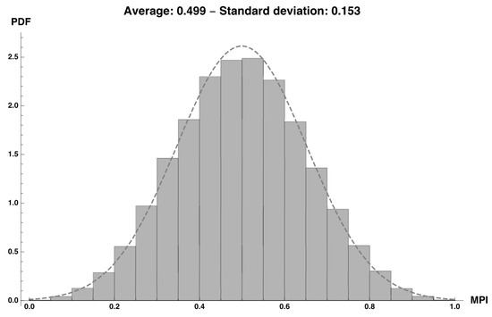
Figure 2.
Results of the first of the five Montecarlo simulations compared to a Normal Distribution with the same average and standard deviation (Dashed line).
Table 4.
Percentiles and Maintenance Priority Index (MPI) values.
The Montecarlo simulation has been carried out in order to be able to define better the thresholds in Table 5. The Probability Density Function (PDF) described in Figure 2 allows us to identify the most likely values according to the values assumed by the four coefficients, therefore it allows us to identify most suitable thresholds for the assessment of the assets.
Table 5.
Thresholds defined for the four metrics of the Decision Support System (DSS).
3.2. The Facility Condition Index in the Decision Support System
The following step concerns the investigation of how the FCI behave in the DSS, since the FCI thresholds and equation have been revised in order to be more suitable for the calculation of the algorithm. Therefore, an evaluation of the variation of the MPI according to the variation of the values of the four parameters has been accomplished. In order to do this, some thresholds have been defined not only for the FCI but also for the other indicator. The thresholds have been defined thanks to the Montecarlo simulation (Figure 2 and Table 4).
For the FCI three levels have been defined: “good”, “fair” and “poor” as suggested in many literature references [16]. For the D index, if the component presents an ASL below the half of the RSL, thus can be classified as in good conditions. If the ASL is between the half of the RSL and the end of the RSL, then the component is in a fair condition, otherwise it can be considered to be in a poor condition, since it means that it is operating with an ASL that is greater than expected. Therefore, it has been operating for a longer period than what is expected in standard conditions. The thresholds defined for the P and the C values are the same. Even in this case, the two parameters are following a similar logic in the evaluation of the priority and criticality assigned to the assets.
Once the thresholds have been identified, some reference values have been defined for the four metrics (Table 6).
Table 6.
Reference values for the four metrics od the Decision Support System DSS.
The following step concerns the definition of the thresholds to be associated to the MPI. The index is composed of four metrics. The values of each metric can be organized in three classes: good, fair, poor (Table 6). For determination of the thresholds a minimum and maximum value of the FCI must be defined. These parameters have been set as described in Table 7.
Table 7.
Facility Condition Index (FCI) and scaled Facility Condition Index (FCI*) values adopted for the definition of the Maintenance Priority Index (MPI) thresholds.
These values of the FCI have been combined with those related to the D, C and P indexes giving as results a combination of 34 = 81 cases. These results have been organized in a table and the thresholds of the MPI have been agreed as shown in Table 8:
Table 8.
Maintenance Priority Index (MPI) thresholds.
Figure 3 represents an example of different combination of the four metrics computed for the calculation of the MPI. Additionally, the central red circle represents the MPI value obtained from the calculation of the four metrics. From top left and clockwise, the circles represent FCI, D, C and P.
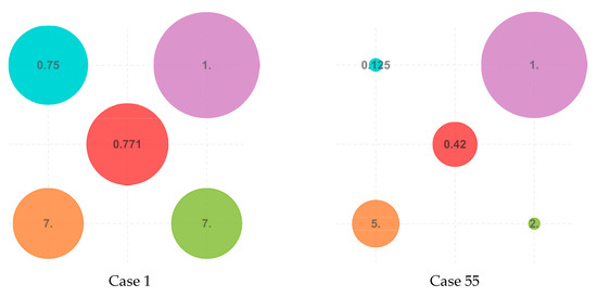
Figure 3.
visualization of the combination of the four metrics composing the Maintenance Priority Index (MPI). The central circle represents the value of the Maintenance Priority Index (MPI).
Once the MPI has been computed for all the assets within the building, the budget allocation can take place. Therefore, assets are ranked in ascending order according to their MPI value. Economic resources are allocated first to those assets with a higher MPI. Maintenance interventions are assigned to assets as long as there is enough budget to implement them. The maintenance interventions and related costs are defined thanks to the calculation of the deferred maintenance (Equation (1)). The proposed algorithm sits in the core of the DSS for maintenance budget allocation.
4. Results
The proposed DSS has been tested and applied in a case study, in order to demonstrate the behavior of the metrics composing the algorithm and for testify its robustness. The following paragraphs describe the outcomes of these analyses and testing procedures.
4.1. The Influence of Criticality (C) and Preference (P) Indicators
The MPI allows us to combine the four indicators and to combine the evaluation of different phenomena in a single performance metric. This aggregation is used to overcome one of the main problems related to FCI and its use in maintenance prioritization, concerning the need for the combination with other metrics. If the priority of maintenance operations is defined only according to the FCI (i.e., an asset with higher FCI will be maintained sooner than the ones with al lower FCI), it will be very probable that assets with low CRV will be maintained first and those with very high CRV will not be considered properly. In fact, FCI is known to be a metric led by the CRV [39].
This gives rise to a question: are P and C indicators enough to change the priority of maintenance given by the only FCI? In order to answer this question a further investigation has been accomplished.
At first the ratio between to MPI of two different assets has been calculated through Equation (9), as function of the CRV ratio and the P ratio:
where:
- is the ratio between the current replacement values of two components;
- is the ratio between the priority indexes of the same two components.
It must be considered that the P and the C indexes impact on the function in the same way. Therefore, the y variable can be defined both considering the ratio between the P or the C index. In this case the ratio between the P indexes of two assets has been considered. The trend of the MPI ratio according to the variation of the ratios of CRV and P ratios is represented in Figure 4. The MPI ratio presents a negative variation when the CRV ratio increases, confirming that the FCI is a metric led by the denominator, which increases when the P ratio increases. This trend confirms that the P and C indexes are effectively impacting on the final outcome of the calculation of the algorithm.
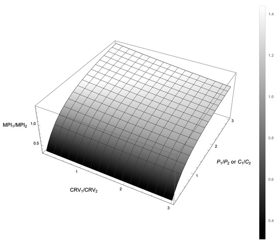
Figure 4.
Ratio between the Maintenance Priority indexes (MPI) of two components according to the ratio of Current Replacement Values (CRV) and Priority index (or Criticality Index).
Table 9 presents the results of an example carried out on two assets. Even in the cases when the FCI would strongly orient towards the implementation of the maintenance interventions on the specific component (CRV1/CRV2 = 0.4 or 1.75), the Priority index (or Criticality index) can lead to completely different situations, compared to the results of the simple FCI. For instance, if two assets present DM1 = DM2 but a CRV1/CRV2 = 0.5, the prioritization of the maintenance interventions based on the FCI would lead to a resource allocation for maintaining the component 1 (FCI1 = 2 FCI2), while the MPI ratio drive the allocation of the same resources on component 1 if P1/P2 >= 1, otherwise on the component 2 (see Table 9). The same considerations can be made using the ratio between the criticality of the two components instead of the one between the preference.
Table 9.
Variation of the Facility Condition Index (FCI) ratio and Maintenance Priority Index (MPI) ratio according to Current Replacement Value (CRV) ratio and Priority index (P) ratio.
4.2. Case Study Results
The proposed DSS has been applied to a case study to test its robustness and the possibility of effectively drive the budget allocation for maintenance interventions. The DSS has been applied to an office building in Erba, in the north of Italy. The building is occupied by a construction company and by a notary firm for a total surface of approx. 3000 sqm. The building was accomplished in 2007 and sits in a piedmont climatic condition (Figure 5). The building has been modeled through Revit with a low Level of Detail (LoD) and a high Level of Information (LoI). However, the DSS has not been completely integrated in the BIM model.
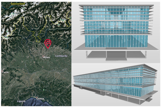
Figure 5.
location (left) and Building Information Model (BIM) model of the office building on which the Decision Support System (DSS) has been implemented.
The first step for the calculation of the algorithm concerns the definition of list of assets to be maintained. This operation is crucial for effective information management framework since it defined the granularity at which maintenance operations take place. The assets have been defined considering the definition provided by the standard ISO 16739-1 [35]. Therefore, elements have been aggregated not only following the location and typological criteria but also following a functional criterion, grouping those elements on which maintenance operations can be carried out uniformly.
These assets have been employed for the development of a standard list of maintenance interventions, collected and used for the definition of their maintenance profiling. Accordingly, the CRV for each asset has been calculated thanks to the use of CAD drawings, technical specifications and 3D models available at the moment of the development of the case study. The CRV costs have been defined according to the Pricelist 2018 published by the Comune di Milano [40] and Camerca di Commercio Milano Monza Brianza Lodi [41]. Once the CRV values have been defined, a condition assessment has been carried out and the deferred maintenance interventions for each asset have been identified. This operation gave as an outcome a list of 246 components with the DM > 0, most of them with a small CRV (Figure 5).
172 assets out of the 246 present a DM smaller than 5000 € for a total amount of 253.908 €. The value of the DM for each of the 246 assets is represented in Figure 6. 69.9% of the 172 DM cost 7.15% of the total cost of DM, amounting to €351.632.

Figure 6.
Histogram of Current Replacement Value (CRV) for the components with Deferred Maintenance (DM) > 0. Most of the component have small CRV.
After the condition assessment, carried out in this case checking the maintenance interventions performed against those defined in the maintenance plan, the MPI can be computed. Figure 7 shows the initial situation, after the condition assessment. For each asset, the colors display how much each of the four metrics (FCI*, D, P, C) contribute to the MPI.

Figure 7.
Maintenance Priority Index (MPI) of the components with Deferred Maintenance (DM) > 0. The colors show how the Facility Condition Index (FCI), D index (measuring the age of the assets), P index (measuring the preference of the owner) and C index (measuring the criticality of each asset) contribute to the MPI of each component.
The mean initial FCI of all the assets is FCIinit = 10.8% (poor) and the corresponding MPIinit is approximately 43.0% (medium). Figure 8 allows us to compare FCIinit and MPIinit. The vertical dashed lines represent the standard limits for poor and fair conditions used in FCI while the horizontal dashed lines are the limits for low and medium priority defined for MPI. It can be seen that some components with a very good FCI have a high MPI due to D, P or C.
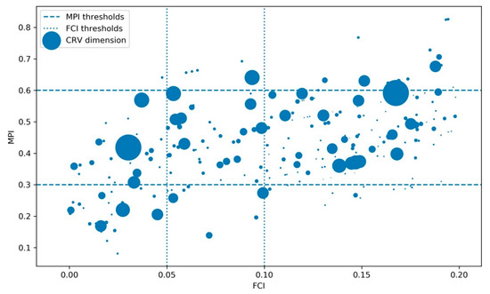
Figure 8.
Comparison between Facility Condition Index (FCI) and Maintenance Priority index (MPI) of the components and dimension of the Current Replacement Value (CRV).
The following stage concerns the budget allocation of reduced resources for the optimization of maintenance operations. For this simulation, it is assumed a budget constrain (B) equal to 65% of the cost of all the DM detected during the condition assessment (Equation (10)).
Limited by this constrain, it is possible to perform maintenance activities only on 130 components chosen according to the MPI from the highest to the lowest possible, according to the budget constrain. The assets have been chosen confronting the cumulative sum of the deferred maintenance with the budget, until the budget is totally spent.
The budget set to 65% of the total DM cost, allows us to solve the deferred maintenance of approximately 130 assets (98% of the total DM of the 130 assets) identified through the MPI ranking. Maintenance interventions carried out, allowed to reduce the average MPI to 34.5%, namely 19.7% less than the initial MPI (Figure 9); whilst the average FCI assume the value of 3.9%, corresponding to a decrease of the FCIinit of 63.7% (Figure 10). The breakdown of values assumed by each metric composing the MPI is shown in Figure 11.

Figure 9.
Maintenance Priority Index (MPI) before (ivory) and after (light grey) maintenance. The dashed line is the average MPI after maintenance, the dotted one is the average MPI before maintenance.

Figure 10.
Facility Condition Index (FCI) before (ivory) and after (light grey) maintenance. The dashed line is the average FCI after maintenance, the dotted one is the average FCI before maintenance.
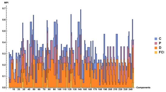
Figure 11.
Maintenance Priority Index (MPI) of the components after the maintenance. The colors show how the Facility Condition Index (FCI), D index (measuring the age of the assets), P index (measuring the preference of the owner) and C index (measuring the criticality of each asset) contribute to the MPI of each component.
Comparing Figure 7 and Figure 11 it is possible to visualize how the maintenance optimization affects ¼ of the MPI, sine it impacts on the reduction of the FCI. This is the only metric of the DSS that is drastically reduced after the prioritization of the maintenance interventions. Figure 11 and Figure 12 demonstrate that some assets present, after the implementation of the maintenance interventions, an FCI = 0, despite the values of the remaining three metrics remain the same. This may cause a situation, as described in Figure 12, where some priority assets still maintain a high value of the MPI, despite the FCI is equal to 0.

Figure 12.
Comparison between Facility Condition Index (FCI) and Maintenance Priority Index (MPI) of the components after maintenance.
Using MPI or FCI to prioritize maintenance leads to completely different results. This because MPI considers also the age of components, their criticality and the priority of the owner / manager of the asset. Figure 13 compares two different maintenance prioritization strategies which can be applied to the same case study with the same budget constraint. One maintenance prioritization strategy is based on MPI, the other is based on the use of FCI. As it can be seen, there is a group of components, the green dots in Figure 13, characterized by high MPI and elevated FCI values that are going to be maintained regardless of the KPI used to set priority. There is another group of assets, identified by the red dots, that using either FCI or MPI, are not going to be maintained. The blue dots represent assets that are going to be maintained only if the priority is set using the FCI. Eventually, the yellow dots are components that need to be maintained if the priority is defined using MPI. In the case study presented in this article, with a maintenance budget set to 65% of the total maintenance needs, if the priority is set using MPI, 130 components out of 246 will be maintained. Otherwise, if FCI is used, 103 components are going to be maintained.

Figure 13.
Assets to be maintained (or not) according to different maintenance prioritization strategies (Facility Condition Index and Maintenance Priority Index computed after the Condition Assessment are shown).
5. Discussion
Based on the results obtained, the DSS has been stressed considering different budget thresholds. A scenario analysis has been carried out, in order to investigate the behavior of the MPI when the budget constraint is changed. If the maintenance budget goes from 55% to 65% of the total cost of the DM the FCI decreases of 36% and the MPI reduction is 7%, while if the budget goes from 55% to 75% the FCI present a 49% reduction and the MPI is reduced by 10% (Figure 14).

Figure 14.
Scenario analysis. How Maintenance Priority Index (MPI) (a) and Facility Condition Index (FCI) (b) change according to the budget constrain expressed in percentage of the Deferred Maintenance (DM) costs.
The scenario analysis demonstrated that increasing the maintenance budget, the MPI decreases slower, since most critical assets are repaired first, thanks to the logic adopted in the development of the maintenance prioritization algorithm.
Influence of Uncertainty of Input Data on MPI
Computing replacement and maintenance costs is fraught with potential errors due to lack of knowledge of the actual condition of the asset to be maintained and of its surroundings. Noteworthy, most of the times these costs are not forecasted by the same person who made the survey for the condition assessment, this leads to estimates characterized by uncertainty. Many authors when forecasting maintenance and life cycle costs suggest dealing with uncertainty using Montecarlo (MC) simulation method: Tae-Hui, K. et al. [42] uses MC simulations to estimate maintenance and repair costs of hospital facilities, Rahman, S. et al. [43] for LCC of municipal infrastructure and Park, M. et al. [44] to analyze aged multi-family housing maintenance costs.
The correct choice of the stochastic inputs for the MC simulation is of paramount importance. In an analysis of building components life cycle costs, Di Giuseppe et al. [45] found that uncertainty in the estimation of the costs of the components (CRV of the assets in this case study), is well modeled using the uniform distribution, Equation (11), with the two limits a and b computed, respectively, as −/+10% of the deterministic costs.
Likewise, Di Giuseppe et al. [45] suggest using a Normal Distribution, Equation (12), for the maintenance costs (in this article the DM costs). The deterministic value of DM has to be used as the mean of the Normal distribution and 3% of the same cost as the standard deviation.
Eventually, the same source [45], suggests using a Uniform distribution with -/+20% of the deterministic ESL as a and b limit to model service life uncertainty while computing D, one of the four KPIs used in the proposed MPI. D, as shown in Equation (5), is the ratio of the actual service life of the component and the estimated one. While most of the times there is no uncertainty in ASL, ESL may be subject to a great variability that can be effectively modeled using the uniform distribution.
Main results of a 10,000 sample MC simulations are presented in Table 10, where mean and standard deviation of both FCI and MPI of the whole building (the mean of the MPI and FCI of all the components) are showed. These values have been compared to the deterministic values, respectively MPI = 0.3446 and FCI = 0.0390. The percentage difference between the mean of MC simulation and the deterministic values is 1.16% for MPI and 9.74% for FCI, demonstrating that the uncertainty on costs and service lives affects mostly the FCI forecast. This is not an unexpected result since costs only affect 25% of MPIs while FCI is totally dependent on them.
Table 10.
Results of the Montecarlo simulation. Mean and standard deviation of Maintenance Priority Index (MPI) and Facility Condition Index (FCI) deterministic values obtained in the case study.
Moreover, Figure 15 represents the probability density curve and cumulative one of the MPI, while Figure 16 represents the same outcome for the FCI. These images allow us to better compare deterministic values with the outcome of the MC simulations. As it can be seen also in Figure 16, the deterministic values computed for MPI and FCI are slightly optimistic, i.e., the uncertainty in costs and service lives will lead to higher values of both the KPIs (Figure 17). Noteworthy, even if the assumed uncertainty is quite high, +/− 20% for the ESL and +/− 10% for the CRV, the final result is slightly affected by it.
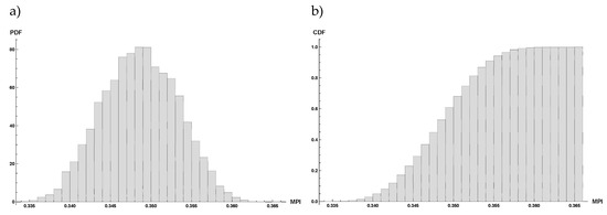
Figure 15.
Montecarlo simulation results. Probability (a) and Cumulative (b) density function of Maintenance Priority Index (MPI).

Figure 16.
Montecarlo simulation results. Probability (a) and Cumulative (b) density function of Facility Condition Index (FCI).
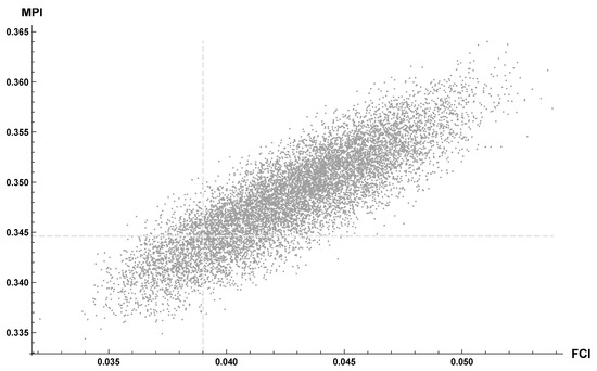
Figure 17.
Combination of Maintenance Priority Index (MPI) and Facility Condition Index (FCI) for each one of the 10,000 simulations compared to the deterministic Maintenance Priority Index (MPI) and Facility Condition Index (FCI) (dashed lines).
The deterministic values of MPI and FCI are close to the average of MC simulations. This means that, with the uncertainty on CRV, DM and RSL assumed to be as described above, there is a 50% probability that the real value of MPI and FCI will be higher than expected. This is a very high probability of error. MPI and FCI values with a lower probability of error, can be taken from Table 11 which shows the quantile of the two KPIs. For example, MPI = 0.3519 and FCI = 0.0452 have a probability of been overcome, i.e., of error, of only 25%, meaning in 75% of the cases, the actual values of the two KPIs will be lower than these.
Table 11.
Results of the Montecarlo simulation. Maintenance Priority Index (MPI) and Facility Condition Index (FCI).
6. Conclusions
Through this research a DSS for maintenance budget allocation on physical assets has been developed and its robustness and applicability has been demonstrated through a case study. The technical assessment of the building has been carried out thanks to the FCI and the D indexes. The former describes, through an economic measure, the maintenance performance of the assets. The latter compares, in a scale 0-1, the ASL of each component to its ESL. Moreover, two non-technical performances related to the building are encompassed in the DSS through two indicators: the criticality (C) of the failure of each asset on the overall building and the maintenance preference (P) of the building owner for each single asset. This allows us to gather phenomena belonging to different domains within the Digital Asset Management context. This cross-domain characterization of the DSS allows us to address the contemporary trends in management of the built environment. The built environment should no longer be defined only through its physical properties, but also through the services that can be provided through its use. Therefore, the DSS is composed of metrics belonging to different domains of the AM discipline.
The definition of the level of aggregation of the components, composing the ifcAssets, on which maintenance interventions are carried out, is a critical issue to be considered in the development of the DSS. This phase is crucial, since it defines the level of aggregation of the information concerning the operation of a physical asset. This generalization of the information is a key factor for management of the asset during its life cycle, since it determines the level at which the information requirements for AM should be provided.
Moreover, some further development of the research can be highlighted. The final calculation of the MPI at the level of the single asset is obtained through the simple average among the four metrics of the MPI (FCI, D, C, P). This result could be different if a weighted average would be carried out. Nevertheless, the definition of the weighting system could lead to completely different results compared to those obtained through the current version of the proposed DSS, adding uncertainty to the DSS computation. The DSS, in fact, already comprehends some preference parameters (D and P), and therefore is partially driven by the choices made by specific subjects working for the correct operation of the building.
In this article the calculation of the MPI at the building level is presented. Once the MPI for each asset within the building has been computed, an average MPI for the whole building can be calculated. However, this value cannot be used for carrying out comparisons among buildings within a portfolio, since the FCI normalization do not allow us to compare same elements in different buildings. Therefore, further research should be accomplished to fill the scalability gap of the DSS.
Within the context of the digitization of the built environment, the DSS could be further integrated into the BIM approach, allowing a stronger integration for data collection and storage in the digital model. Therefore, further research will be done in the field of information requirements for using AM and FM to exploit the digital tools for information management. This could provide a further proof of the effectiveness in the implementation of BIM methodologies in AM and FM, towards the definition of a Digital Twin of the built environment. Moreover, the aggregation of the building components through the use of the ifcAsset definition, facilitate the integration of the DSS in a BIM environment [46,47]. Thanks to the flexibility in the definition of the level of aggregation at which maintenance interventions are applied, the DSS allows us to address the issue of portfolio management and infrastructural asset management. However, when the DSS is applied to a different scale, the inclusion of the location in the algorithm becomes a crucial issue. Therefore, further parameters could be included in the DSS, allowing the prioritization of the maintenance interventions, according to location-based metrics. The employment of the DSS at the portfolio or infrastructural level opens new research questions concerning how to integrate GIS and BIM for effective asset and facility management. Therefore, the scope of the research should be expanded to the GeoBIM Asset and Facility Management [48]. Further metrics could be included in the algorithm, as it is able to catch cross-domain issues, despite being based on only few KPIs.
Author Contributions
F.R.C.: Conceptualization, Methodology, Supervision, Visualization, Writing—original draft, Writing—review & editing. N.M.: Conceptualization, Methodology, Visualization, Writing—original draft, Writing—review & editing.
Funding
This research receives no external funding.
Acknowledgments
Authors would like to express their gratitude to Rigamonti Francesco S.p.A. for funding part of the Nicola Moretti’s scholarship.
Conflicts of Interest
The authors declare no conflict of interest.
Abbreviations
| AIM | Asset Information Model |
| AM | Asset Management |
| API | Asset Priority index |
| ASL | Actual Service Life |
| BIM | Building Information Modeling |
| C index | Criticality index is a KPI measuring the criticality as the consequence of the failure of the component, for the effective execution of the core business of the organization occupying the asset |
| CA | Condition Assessment |
| CAFM | Computer Aided Facility Management |
| CAD | Computer Aided Design |
| CIcomp | Composed Condition Index |
| CMMS | Computerized Maintenance Management Systems |
| CRV | Current Replacement Value |
| D index | KPI measuring the service life of the asset (building component) |
| DM | Deferred Maintenance |
| DoI | Department of Interior |
| DSS | Decision Support system |
| FM | Facility Management |
| FCI | Facility Condition Index |
| FCIcomp | Composed Facility Condition Index |
| IWMS | Integrated Workplace Management Systems |
| KPI | Key Performance Indicator |
| LoD | Level of Detail |
| LoI | Level of Information |
| MC | Montecarlo method |
| MPI | Maintenance Priority index |
| NACUBO | National Association of College and University Business Officers |
| P index | Priority index is a KPI measuring the preference of the asset owner, in the perspective of the execution of the core business |
| Probability Density Function | |
| RSL | Reference Service Life |
| USA | United States of America |
References
- Amaratunga, D.; Haigh, R.; Sarshar, M.; Baldry, D. Application of the Balanced Score-card Concept to Develop a Conceptual Framework to Measure Facilities Management Performance within NHS Facilities. Int. J. Health Care Qual. Assur. 2002, 15, 141–151. [Google Scholar] [CrossRef]
- Nical, A.K.; Wodynski, W. Enhancing Facility Management Through BIM 6D. Procedia Eng. 2016, 164, 299–306. [Google Scholar] [CrossRef]
- Brochner, J.; Haugen, T.; Lindkvist, C. Shaping Tomorrow’s Facilities Management. Facilities 2019, 37, 366–380. [Google Scholar] [CrossRef]
- Saxon, R.; Robinson, K.; Winfield, M. Going Digital. A Guide for Construction Clients, Building Owners and Their Advisers; UK BIM Alliance: London, UK, 2018. [Google Scholar]
- Volk, R.; Stengel, J.; Schultmann, F. Building Information Modeling (BIM) for Existing Buildings-literature Review and Future Needs. Autom. Constr. 2014, 38, 109–127. [Google Scholar] [CrossRef]
- Chen, W.; Chen, K.; Cheng, J.C.P.; Wang, Q.; Gan, V.J.L. BIM-based Framework for Automatic Scheduling of Facility Maintenance Work Orders. Autom. Constr. 2018, 91, 15–30. [Google Scholar] [CrossRef]
- Mcarthur, J.J. A Building Information Management (BIM) Framework and Supporting Case Study for Existing Building Operations, Maintenance and Sustainability. In Proceedings of the International Conference on Sustainable Design, Engineering and Construction, Chicago, IL, USA, 10–13 May 2015; Volume 118, pp. 1104–1111. [Google Scholar]
- Moretti, N.; Dejaco, M.C.; Maltese, S.; Re Cecconi, F. The Maintenance Paradox. ISTEA 2017-Reshaping Constr. Ind. 2017, 234–242. [Google Scholar]
- Luoto, S.; Brax, S.A.; Kohtamaki, M. Critical Meta-analysis of Servitization Research: Constructing a Model-narrative to Reveal Paradigmatic Assumptions. Ind. Mark. Manag. 2017, 60, 89–100. [Google Scholar] [CrossRef]
- Vandermerwe, S.; Rada, J. Servitization of Business: Adding Value by Adding Services. Eur. Manag. J. 1988, 6, 314–324. [Google Scholar] [CrossRef]
- Lavy, S.; Garcia, J.A.; Dixit, M.K. KPIs for Facility’s Performance Assessment, Part I: Identification and Categorization of Core Indicators. Facilities 2014, 32, 256–274. [Google Scholar] [CrossRef]
- Alexander, K. Facilities Management Practice. Facilities 1992, 10, 11–18. [Google Scholar] [CrossRef]
- Amaratunga, D.; Baldry, D. Assessment of Facilities Management Performance in Higher Education Properties. Facilities 2000, 18, 293–301. [Google Scholar] [CrossRef]
- Yang, H.; Yeung, J.F.Y.; Chan, A.P.C.; Chiang, Y.H.; Chan, D.W.M. A Critical Review of Performance Measurement in Construction. J. Facil. Manag. 2010, 8, 269–284. [Google Scholar] [CrossRef]
- Ladiana, D. Manutenzione e Gestione Sostenibile Dell’ambiente Urbano; Alinea Editrice: Firenze, Italy, 2007. [Google Scholar]
- Dejaco, M.C.; Re Cecconi, F.; Maltese, S. Key Performance Indicators for Building Condition Assessment. J. Build. Eng. 2017, 9, 17–28. [Google Scholar] [CrossRef]
- ISO. ISO 41011:2017. Facility Management-Vocabulary; ISO: Geneva, Switzerland, 2017. [Google Scholar]
- Amaratunga, D.; Baldry, D.; Sarshar, M. Assessment of Facilities Management Performance. Facilities 2000, 18, 258–266. [Google Scholar] [CrossRef]
- Amaratunga, D.; Baldry, D. A Conceptual Framework to Measure Facilities Management Performance. Prop. Manag. 2003, 21, 171–189. [Google Scholar] [CrossRef]
- Parn, E.A.; Edwards, D.J.; Sing, M.C.P. The Building Information Modeling Trajectory in Facilities Management: A Review. Autom. Constr. 2017, 75, 45–55. [Google Scholar] [CrossRef]
- Rush, S.C. Managing the Facilities Portfolio: A Practical Approach to Institutional Facility Renewal and Deferred Maintenance; National Association of College and University Business Officers: Washington, DC, USA, 1991. [Google Scholar]
- Lavy, S.; Garcia, J.A.; Dixit, M.K. Establishment of KPIs for Facility Performance Measurement: Review of Literature. Facilities 2010, 28, 440–464. [Google Scholar] [CrossRef]
- Lavy, S.; Garcia, J.A.; Dixit, M.K. KPIs for Facility’s Performance Assessment, Part II: Identification of Variables and Deriving Expressions for Core Indicators. Facilities 2014, 32, 275–294. [Google Scholar] [CrossRef]
- Maltese, S.; Dejaco, M.C.; Re Cecconi, F. Dynamic Facility Condition Index Calculation for Asset Management. In Proceedings of the 14th International Conference on Durability of Building Materials and Components, Ghent, Belgium, 29–31 May 2017. [Google Scholar]
- U.S. Department of Interior. U.S. Department of Interior Policy on Deferred Maintenance, Current Replacement Value and Facility Condition Index in Life-Cycle Cost Management; U.S. Department of Interior: Washington, DC, USA, 2008.
- U.S. Department of Interior. U.S. Department of Interior Management Plan. Version 3.0; U.S. Department of Interior: Washington, DC, USA, 2008.
- U.S. Department of Interior. U.S. Department of Interior National Park Service Park Facility Management Division Park Facility Management Division; U.S. Department of Interior: Washington, DC, USA, 2012.
- U.S. Department of Interior. U.S. Department of Interior Deferred Maintenance and Capital Improvement Planning Guidelines; U.S. Department of Interior: Washington, DC, USA, 2016.
- IFMA. Asset Lifecycle Model for Total Cost of Ownership Management. Framework, Glossary Definitions. In A Framework for Facilities Lifecycle Cost Management; IFMA: Houston, TX, USA, 2008. [Google Scholar]
- U.S. Department of Interior. U.S. Department of Interior Site-Specific Asset Business Plan (ABP) Model Format Guidance; U.S. Department of Interior: Washington, DC, USA, 2005.
- Lavy, S.; Garcia, J.A.; Scinto, P.; Dixit, M.K. Key Performance Indicators for Facility Performance Assessment: Simulation of Core Indicators. Constr. Manag. Econ. 2014, 32, 1183–1204. [Google Scholar] [CrossRef]
- U.S. Department of Interior. U.S. Department of Interior Asset Priority Index Guidance; U.S. Department of Interior: Washington, DC, USA, 2005.
- Mills, C.D. An Evaluation of U.S. Coast Guard Shore Facility Readiness Measures; U.S. Army War College, Strategy Research Project: Carlisle, PA, USA, 2001. [Google Scholar]
- NASA. The NASA Deferred Maintenance Parametric Estimating Guide; National Aeronautics and Space Administration: Washington, DC, USA, 2003.
- ISO. ISO 16739-1:2018-Industry Foundation Classes (IFC) for Data Sharing in the Construction and Facility Management Industries-Part 1: Data Schema; ISO: Geneva, Switzerland, 2018. [Google Scholar]
- ISO BS EN. ISO 19650-2:2018. Organization and Digitization of Information about Buildings and Civil Engineering Works, Including Building Information Modeling (BIM)-Information Management using Building Information Modeling. Part 2: Delivery Phase of the Assets; ISO: Geneva, Switzerland, 2018. [Google Scholar]
- ISO. ISO 15686-1:2011 Buildings and Constructed Assets-Service Life Planning-Part 1: General Principles and Framework; ISO: Geneva, Switzerland, 2011. [Google Scholar]
- US Department of Defense MIL-STD-1629A. Military Standard. Procedures for Performing a Failure Mode, Effects and Criticality Analysis; Department of Defense: Washington, DC, USA, 1980.
- Re Cecconi, F.; Moretti, N.; Dejaco, M.C. Measuring the Performance of Assets: A Review of the Facility Condition Index. Int. J. Strateg. Prop. Manag. 2019, 23, 187–196. [Google Scholar] [CrossRef]
- Comune di Milano. Listino Prezzi Comune di Milano. Edizione 2018. Available online: http://www.comune.milano.it/wps/portal/ist/it/amministrazione/trasparente/OperePubbliche/listino_Prezzi/Edizione%2B2018 (accessed on 17 March 2019).
- Camera di Commercio Milano Monza Brianza Lodi Home-PiùPrezzi, Il portale dei prezzi della Camera di Commercio di Milano. Available online: http://www.piuprezzi.it/ (accessed on 13 May 2019).
- Tae-Hui, K.; Jong-Soo, C.; Young Jun, P.; Kiyoung, S. Life Cycle Costing: Maintenance and Repair Costs of Hospital Facilities Using Monte Carlo Simulation. J. Korea Inst. Build. Constr. 2013, 13, 541–548. [Google Scholar]
- Rahman, S.; Vanier, D. Life Cycle Cost Analysis as a Decision Support Tool for Managing Municipal Infrastructure Building Regulation-Standards Processing View Project Municipal Infrastructure Investment Planning View Project; In-House Publishing: Rotterdam, The Netherlands, 2004. [Google Scholar]
- Park, M.; Kwon, N.; Lee, J.; Lee, S.; Ahn, Y. Probabilistic Maintenance Cost Analysis for Aged Multi-family Housing. Sustainability 2019, 11, 1843. [Google Scholar] [CrossRef]
- Di Giuseppe, E.; Massi, A.; D’Orazio, M. Probabilistic Life Cycle Cost Analysis of Building Energy Efficiency Measures: Selection and Characterization of the Stochastic Inputs through a Case Study. Procedia Eng. 2017, 180, 491–501. [Google Scholar] [CrossRef]
- Re Cecconi, F.; Moretti, N.; Maltese, S.; Tagliabue, L.C. A BIM-Based Decision Support System for Building Maintenance. In Advances in Informatics and Computing in Civil and Construction Engineering; Springer International Publishing: Cham, Germany, 2019; pp. 371–378. [Google Scholar]
- Maltese, S.; Branca, G.; Re Cecconi, F.; Moretti, N. Ifc-based Maintenance Budget Allocation. In Bo 2018, 9, 44–51. [Google Scholar]
- Ellul, C.; Stoter, J.; Harrie, L.; Shariat, M.; Behan, A.; Pla, M. Investigating the State of Play of Geobim Across Europe. ISPRS-Int. Arch. Photogramm. Remote Sens. Spat. Inf. Sci. 2018, XLII-4/W10, 19–26. [Google Scholar] [CrossRef]


© 2019 by the authors. Licensee MDPI, Basel, Switzerland. This article is an open access article distributed under the terms and conditions of the Creative Commons Attribution (CC BY) license (http://creativecommons.org/licenses/by/4.0/).