The Energy Impact in Buildings of Vegetative Solutions for Extensive Green Roofs in Temperate Climates

Abstract

Many bibliographical studies have highlighted the positive effects of green roofs as technological solutions both for new and renovated buildings. The one-year experimental monitoring campaign conducted has investigated, in detail, some aspects related to the surface temperature variation induced by the presence of different types of vegetation compared to traditional finishing systems for flat roofs and their impact from an energy and environmental point of view. The results obtained underlined how an appropriate vegetative solution selection can contribute to a significant reduction of the external surface temperatures (10 °C–20 °C for I > 500 W/m² and 0 °C–5 °C for I < 500 W/m², regardless of the season) compared to traditional flat roofs. During the winter season, the thermal gradients of the planted surface temperatures are close to zero compared to the floor, except under special improving conditions. This entails a significant reduction of the energy loads from summer air conditioning, and an almost conservative behavior with respect to that from winter heating consumption. The analysis of the inside growing medium temperatures returned a further interesting datum, too: the temperature gradient with respect to surface temperature (annual average 4 °C–9 °C) is a function of solar radiation and involves the insulating contribution of the soil.

1. Introduction

In support of the choice of green roofs as technological solutions, both for new and renovated buildings, numerous positive effects are cited in the literature, such as the reduction of annual conditioning energy consumption related to heating and cooling [1,2,3], more sensitive in low or moderately insulated buildings [4,5]; aesthetics improvement [2]; noise absorption [6,7,8]; contribution to the reduction of greenhouse gases and urban smog [9]; improvement of air quality with positive effects on human health [10,11]; contribution to the control of urban canyon temperatures [12]; adding up to both thermal insulation and inertia of roof systems, even without completely replacing the thermal insulation [13]; and management of storm water in urban environments [2,14].

This study, considering both the strong effect of roofing systems on the city thermal balance [15] and information relating to some outstanding research issues [16], explores aspects related to the change of surface temperatures induced by the presence of different types of plant species [17,18,19] with respect to a traditional roof finishing system (in particular, a floating floor made of cement-based tiles) and the relationship between different vegetative solutions and the inside temperatures of the growing medium, thus highlighting the influence of green roofs compared to the following aspects:

• reduction of summer thermal loads: during the summer season, the shading induced by plant species [18,20] causes a reduction of surface temperatures [20,21], and a resulting reduction of both indoor temperatures [2,21], and energy consumptions related to the cooling of indoor rooms located below the roofing system [2,21];
• reduction of building materials surface temperature peaks caused by direct solar radiation and concomitant reduction of surface thermal fluctuations [21,22,23]: this corresponds to an increased durability of roofing system materials (such as waterproof roofing membranes);
• reduction of surface temperatures and consequent reduction of radiation phenomena as the basis of the urban heat island effect (UHI) [24,25];
• evaluation of the energy behavior in winter [26], during which the reduction of solar heat gains could cause an increase in heating loads as a function of the reference climatic zone [1]. This implies that the design of the roofing system should be carefully studied in order to correctly size the thickness of both the growing medium and the insulating layer in order to obtain a positive balance even during the winter season.

The positive influence of green roofs is even more sensitive in building refurbishment. Old buildings, for example, are often low or moderately insulated and green roofs can be beneficial in reducing annual conditioning energy consumptions and in adding up to both thermal insulation and inertia of the existing roof system.

2. Method: The Experimental Campaign

2.1. Description of the Experimental Setup

The experimental campaign was carried out on the roof terrace of Fondazione Minoprio (Figure 1), located in the municipality of Vertemate con Minoprio (45°43′18″N–9°04′57″E, climatic zone E [27]).

The monitoring measurement campaign lasted 10 months (from 23 July 2014 to 10 May 2015) and was focused on three different plant species, selected as a function of specific characteristics described in Section 2.2. The choice of plant species: Sedum album, Cerastium biebersteinii, and Phlomis fruticosa.

The 3 m × 3 m experimental area, with a growing medium 10 cm in depth, is placed on the paved surface of the terrace and is contained in a wooden frame covered with non-woven fabric which drains water with no leakage of the growing medium.

The terrace and the conference room located below the terrace underwent renovation from 2005–2007: therefore, the stratigraphy of the terrace meets the thermal insulation requirements of the national legislation in force at the moment of the renovation works [28], which does not substantially affect the monitored thermal behavior of the experimental set-up.

The area is divided into nine plots (1 m × 1 m): in order to validate the monitoring measurements, each plant species was planted three times in three different plots (Figure 2). Forty, 30, and 20 plants were planted for Sedum, Cerastium, and Phlomis, respectively, in order to partially cover the nine plots, awaiting the full potential development.

The random position of the three plots for each plant species was deliberately chosen to ensure, through average data, the reduction and limitation of behavior discrepancies due to the boundaries of the test area.

An emergency irrigation system, consisting of a dropline ensuring a uniform distribution of the water, made of tubes of 16 mm diameter and drippers 20 cm away from one another, was provided. This system is capable of delivering 1.14 liters/h, at the rated drip rate, as a function of pressure. The flow meter is set at approximately 0.55 bars; therefore, at 5.10 Lm/h and 0.7 bar, the final flow rate is equal to 5.7 Lm/h. Three hoses per block were envisaged.

During the first monitoring week (23–27 July 2014) the emergency irrigation system was activated on three different occasions. However, the summer of 2014 was quite rainy and no further operation was planned for the system and was, therefore, shut down.

2.2. The Choice of Plant Species

The ecology of a green roof is similar to a xerophytic environment, characterized by high intensity of direct solar radiation and scarce water availability. Plant species best suited to those contexts often belong to xerophytic, rocky Mediterranean, or mountain environments, in situations of poor water retention and strong wind exposure. Green roofs, even when built in North European climatic zones, refer to this kind of environment due to the poor water retention capacity of the soil, wind exposure, and solar radiation [29]. The most widespread technology north of the Alps is based on Sedum Album, an native Italian species that can live up to 1600 m in altitude and able to survive intense cold.

Three are the species suited to the climate of North Italy belonging to xerophytic environments: Sedum Album, Cerastium biebersteinii, and Phlomis fruticosa.

Sedum Album is suitable to grow in rocky environments, thanks to its CAM (Crassulacean Acid Metabolism) photosynthetic operation; it is characterized by low water consumption [30] and ability to withstand long periods of drought; furthermore, the gaseous exchanges in which leaves absorb CO₂ occur at night so that perspiration is as low as possible. The plants of this species have a creeping growth habit (as it grows at heights between 5 and 10 cm), so the air layer protected by vegetation is very thin.

Cerastium biebersteinii is native of Crimea, but various species of it are also found in Italy, belonging to Cerastium tomentosum group [31]; however, it differs from this group due to a dense hairiness and silver staining. Cerastium biebersteinii offers a better ornamental aspect and a stronger resistance to drought [20]: the habitat to which it belongs is, in fact, the arid Caucasian mountains environment. Even though it has a creeping growth habit, it is more erect than Sedum album and creates large niches under the cover.

Phlomis fruticosa is the tallest plant species, capable of reaching 50 cm in height, and even more in favorable conditions. The large and well-expanded leaves have an attitude to increase perspiration, although no indications are given about its water consumption potential. On the basis of echo physiological parameters, such as the correlation of the voltage with the xylem hydraulic conductance, Iovi [32] argues that the semi-deciduous species Phlomis fruticosa are able to withstand periods of water scarcity, taking advantage, for its growth, of seasons characterized by a greater availability of water.

2.3. The Monitoring System

The monitoring system consists of two TMF500 data loggers (NESA srl, Vidor, Treviso, Italy) [33] housed in special cases. Each acquisition unit can control up to a maximum of 20 cable-connected sensors and it has been configured including all of the information necessary for data transmission, such as acquisition timing and data transmission. The monitoring system reads instantaneous data as a function of the sampling frequency set; subsequently, the data average is calculated to obtain a single datum representing the established sampling interval. In this specific case, a 30-s detection frequency and 5-m single-datum processing were set.

Sensors, wired to the two acquisition units are functional to the monitoring of the growing plots’ performances, to define some experimental setup parameters such as: inside temperatures (T_i), growing medium relative humidity (RHgm), surface temperatures (T_s), underneath growing medium temperatures (T_un), and outside air temperatures (T_a) at a height of 30 cm from the cultivation surface. Figure 3 shows the monitoring scheme. The outdoor air temperature (T_a) sensors are installed only in Q1, Q4, and Q7 plots (see Figure 2a,b).

A surface temperature sensor installed on the flat roof (T_sfloor), on which the experimental area was set up was added, to allow comparisons with the vegetative surfaces data (Figure 4).

A meteorological station was installed near the experimental area in order to monitor the outside climatic conditions; the acquisition system is composed of a TMF500 data logger [33] and the sensors used for detecting the following values: external air temperature (T_e), and relative humidity (RH); global solar radiation (I); and a taco-anemometer for measuring wind direction and speed. In addition to the data provided by the installed weather station, precipitation data were also collected by using a rain gauge owned by Fondazione Minoprio and installed in close proximity to another building of the foundation.

3. Results and Discussions

3.1. Description of the Experimental Setup

Monitoring results were analyzed on a seasonal basis.

Table 1. Main outdoor environmental parameters (external temperatures: minimum (Min), maximum (Max), average (Avg); global solar radiation: maximum (Max), average (Avg); and precipitation: cumulated (Cumul.), Days_rain/Days_tot) typical of the monitored period.

Configuration	Period	External Temperature (°C)			Global Solar Radiation (W/m2)		Precipitations
		Min	Max	Avg	Max	Avg	Cumul. (mm)	Daysrain/Daystot (%)
Summer 2014	23.07–22.09	11.36	31.42	20.36	962	395	316	46
Autumn 2014	23.09–22.12	−1.18	27.11	11.41	768	228	642	54
Winter 2014–2015	23.12–20.03	−5.31	19.47	5.22	702	269	225	33
Spring 2015	21.03–10.05	0.97	28.93	14.54	983	429	124	38

summarizes the main weather characteristics for the four monitoring seasons.

The behavior of the external environmental parameters, monitored from July 2014 to May 2015 and reported in Table 1, compared to those analyzed by ENEA (Italian National Agency for New Technologies, Energy and Sustainable Economic Development) [34], is in line with the expectations with respect to the temperatures and solar radiation. However, as far as precipitation is concerned, the monitored data show a very rainy autumn.

For each of the tabled configurations, some reference weeks and days were chosen to show the main monitored results, divided into two periods of analysis as a function of similar main outdoor average characteristics: summer 2014/spring 2015; autumn 2014/winter 2014–2015.

The decision-making process that led to the choice of the reference weeks and days was based on the following considerations:

• definition of the ‘average weeks’, to limit climatic boundary conditions with the previous and following season, for each configuration period (Table 1);
• definition of the ‘reference weeks’ as the ones characterized by seasonal limit behavior related to external parameters such as solar radiation level, precipitations, high external temperatures; and
• definition of the ‘reference days’ as the ones characterized by similar outdoor conditions in terms of external temperature (28 °C–30 °C peak for the summer 2014/spring 2015 configuration; 13 °C peak for the autumn 2014/winter 2014 configuration) and solar radiation level (900 W/m² for the summer 2014/spring 2015 configuration, and 400–500 W/m² for the autumn 2014/winter 2014–2015 configuration).

The experimental campaign compares the energy and environmental performances of three different plant species: Sedum, Cerastrium, and Phlomis. For this reason, each plant species was planted three times in three different plots, in random positions (Figure 2), to ensure the reduction of discrepancies in the behavior due to the boundaries of the test area.

The results presented and commented below correspond to the average data of the three plots per plant species.

3.1.1. Summer 2014 and Spring 2015

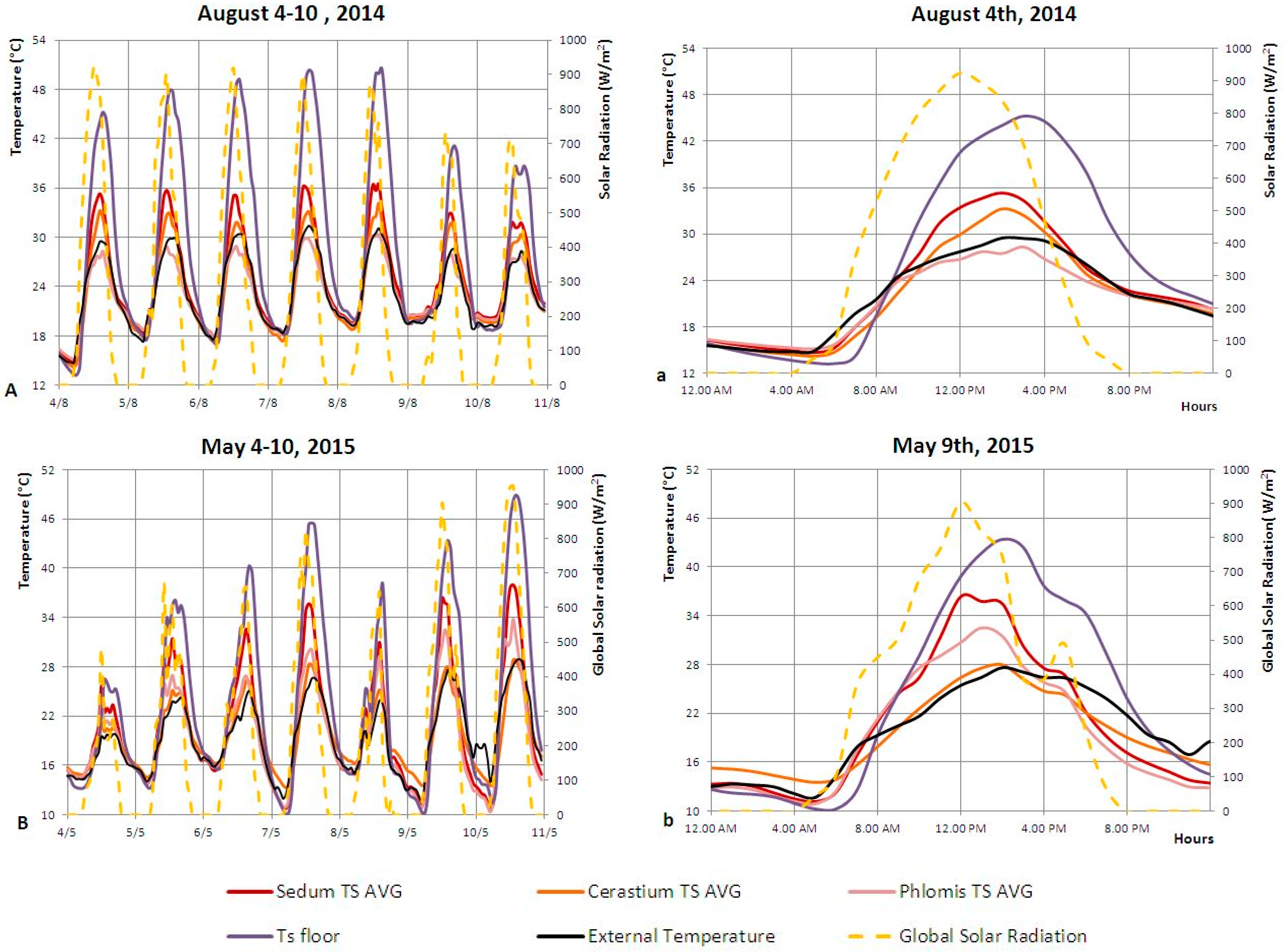
Figure 5 shows graphs concerning the surface temperature of the three plant species (T_s), as a function of the main outside parameters (external temperature and global solar radiation) with respect to two sample weeks, from 4–11 August 2014 (Figure 5A,a), exemplifying summer of 2014, and from 4–11 May 2015 (Figure 5B,b) for spring 2015.

The comparison of performances after one year is focused in order to highlight the incidence of leaf development and shading capacity of each plant species, under the same external conditions.

Graphs of Figure 5 show how the surface temperature of the plant species (T_s), due to its high values, is a function of the solar radiation and it strongly depends on the shading ability of the three plant species. Due to its greater vertical development and greater leaf surface, right from the beginning of the experimental campaign Phlomis offers better shading of the sensors, resulting in a surface temperature (T_s) which is significantly lower (Figure 5a): on 4 May 2014, Phlomis surface temperature T_s is 7.8 °C lower than Sedum and 5.6 °C lower than Cerastium. However, considering next spring (Figure 5b), Cerastium increases its performances: on 9 May 2015, its T_s is 10 °C lower than Sedum and 4.3 °C than Phlomis. The differences in T_s thermal gradients monitored over a year are mainly dependent on the plant leaf development of the three different plant species: Cerastium thickens considerably, while Phlomis tends to dry in the root stock.

Furthermore, by virtue of the different shading attitudes, Cerastium shows a slight phase shift (about 2 h) with respect to the other two species in the attainment of the T_s peak value (Figure 5b).

A correlation index, the Pearson product-moment correlation coefficient (Pearson’s r), was introduced to better understand, on the one hand, the relationship between the global solar radiation (I) and the plant species surface temperatures (T_s) and, on the other hand, the relationship between the external temperature (T_e) and the surface temperatures of the plant species (T_s).

The correlation indexes, summarized in

Table 2. The Pearson product-moment correlation coefficient between (T_s) and (I), and between (T_s) and (T_e), calculated considering three global solar radiation intervals.

Pearson’s r	Global Solar Radiation
between Ts and I	0–200 W/m2	400–600 W/m2	800–1000 W/m2
Sedum	0.79	0.99	0.39
Cerastium	0.78	0.96	0.35
Phlomis	0.83	0.99	0.28
between Ts and Te
Sedum	0.96	0.88	0.25
Cerastium	0.96	0.98	0.74
Phlomis	0.97	0.93	0.26

, were calculated considering three different global solar radiation intervals daily (0–200, 400–600, and 800–1000 W/m², respectively) at solar peak. A sampling period of 41 days was considered (months of August 2014 and May 2015).

The analysis of the correlation index between the surface temperatures of the plant species (T_s) and the external temperature (T_e) shows a direct correlation (Pearson’s r > 0) between them and, at the same time, underlines how the more the global solar radiation increases the more the correlation between (T_s) and (T_e) decreases. Moreover, the correlation between the surface temperatures of the plant species (T_s) and the global solar radiation (I) is direct, increasing, and sensitive (0.8 < Pearson’s r < 1) between 100 W/m² and 800 W/m²; on the contrary, considering very high values of global solar radiation (I > 800 W/m²) the correlation is less sensitive.

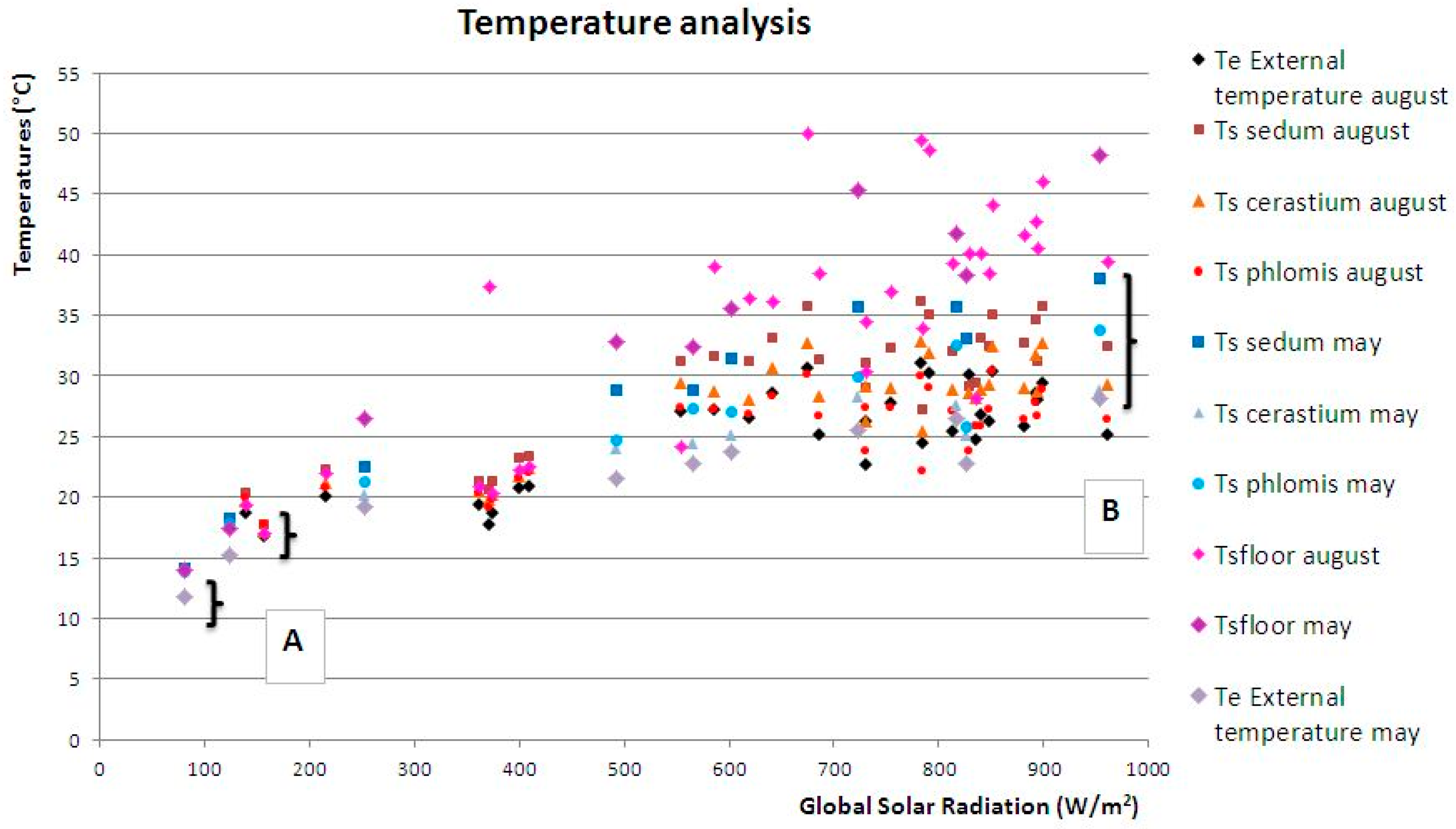
Instead, Figure 6 shows the relationship, in terms of thermal gradients, between the surface temperatures of the plant species (T_s), external temperature (T_e) and global solar radiation (I), during solar peak time, (about 1:30 p.m.). The considered sampling period is 41 days (months of August 2014 and May 2015 -first ten days-).

The surface temperatures of the plant species (T_s) differ from the external temperature (T_e) with a thermal gradient on average lower than 5 °C (‘A’ data in Figure 6) for low values of solar radiation (I < 500 W/m²). Therefore, surface temperatures of the plant species (T_s) differ from the external temperature (T_e) with thermal gradients comprised between 15 °C and 20 °C (‘B’ data in Figure 6) for high values of solar radiation (I > 500 W/m²).

Therefore, the external temperature (T_e) affects the seasonal peak value of the surface temperature of the plant species (T_s), while the global solar radiation determines the thermal gradient between T_s and T_e.

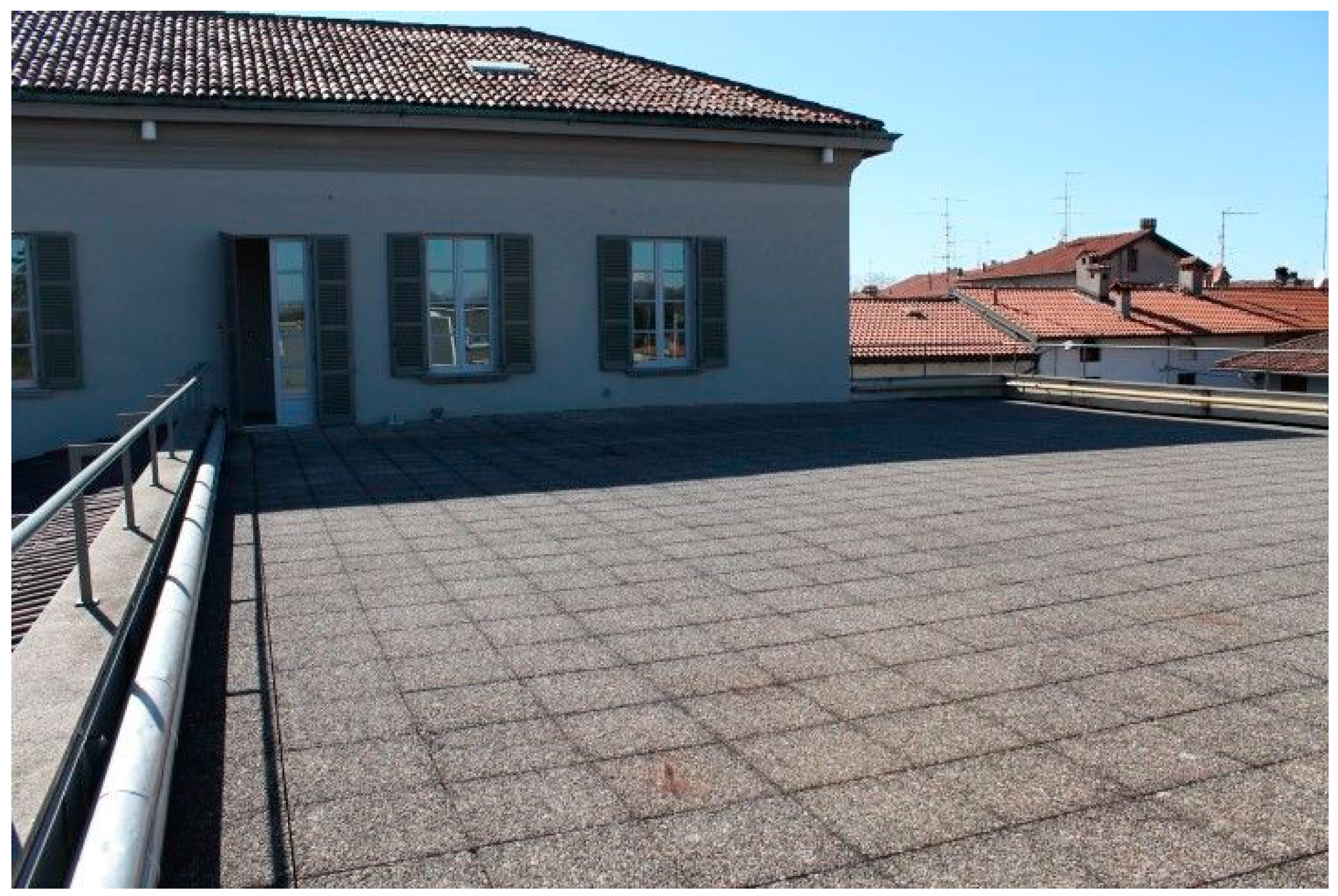
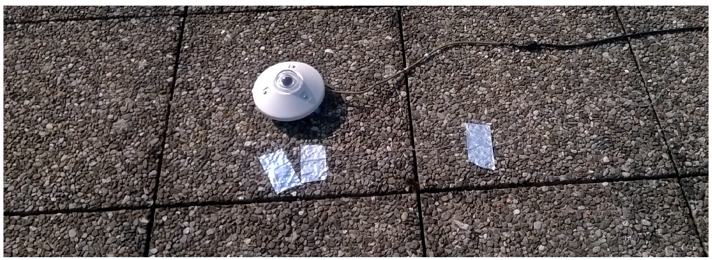
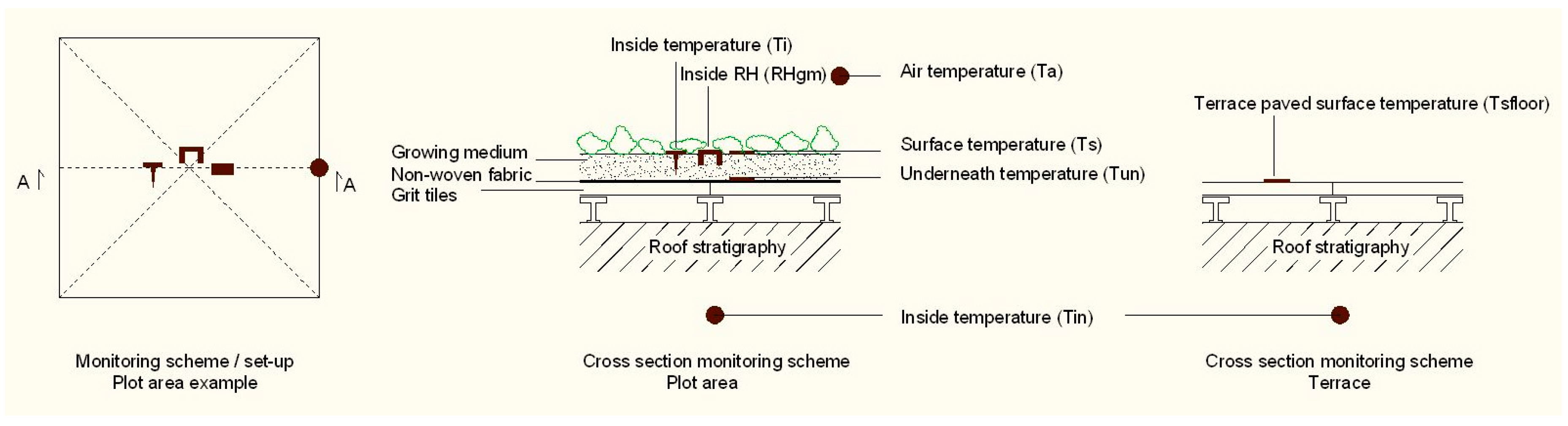
Furthermore, all of the samples of Figure 5 and Figure 6 show how the performances improvement with respect to the paved surface (T_sfloor) of the terrace on which the experimentation is carried out, covered with grey finished grit tiles (Figure 1), is quantified as shown in

Table 3. Surface thermal gradients between surface temperature of the plant species (T_s) and paved surface temperature (T_sfloor), 4 August 2014 and 9 May 2015.

Ts	Sedum	Cerastium	Phlomis	Year
Ts−Tsfloor	−10	−12	−17	2014
Ts−Tsfloor	−7	−15	−11	2015

.

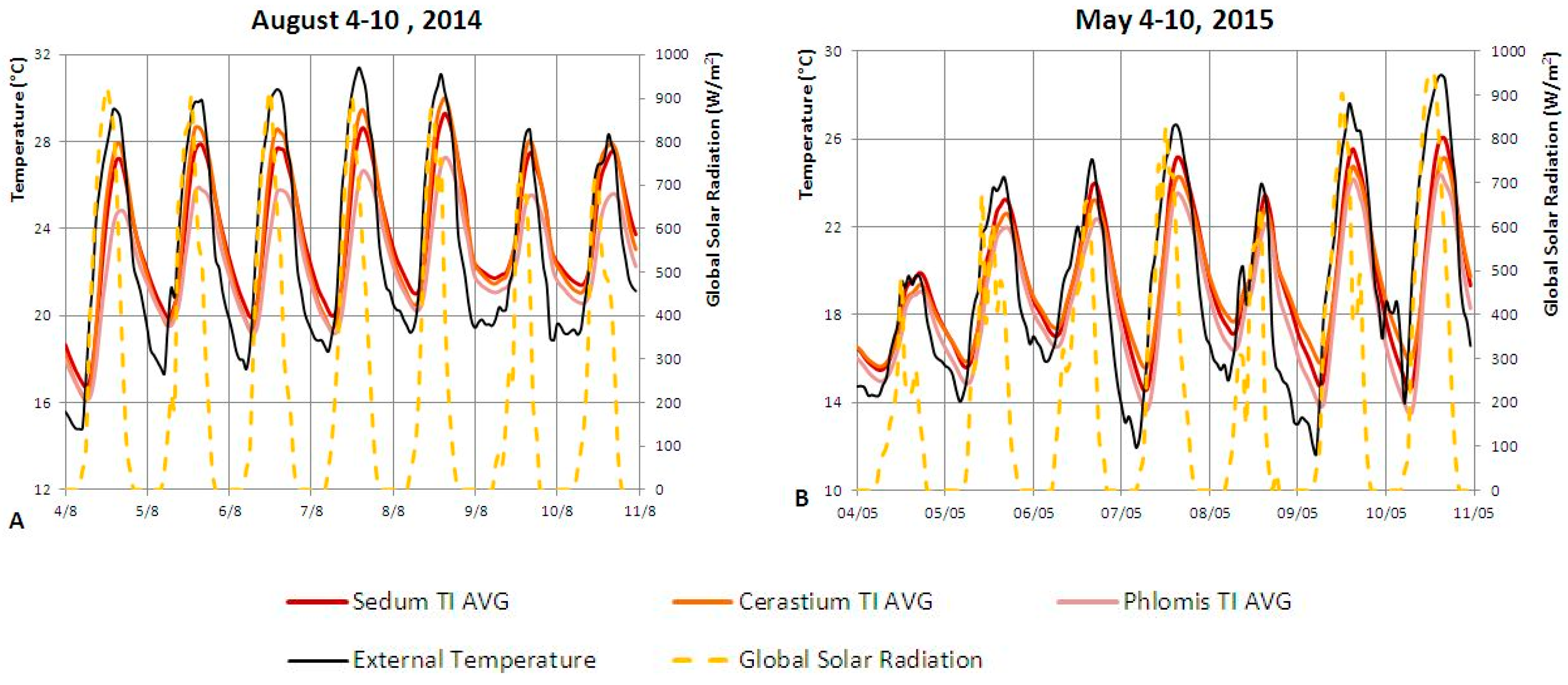
As to the monitoring of the inside temperatures of the growing medium (T_i), measured at a depth of 8 cm, Figure 7 shows trends as a function of both the global solar radiation (I) and the external temperature (T_e) related to 2014 (Figure 7A) and 2015 (Figure 7B), respectively.

The analysis of the inside temperature of the growing medium (T_i) leads to the following considerations: in general, T_i follows the solar radiation trend with an hourly phase displacement similar to the outdoor temperature variation and is affected by the solar shading potential of each plant species (as a function of leaf development and stem high). The trend of Phlomis T_i is in accordance with the expectations, with values 2.5 °C lower than Sedum, while the behavior of Sedum and Cerastium reverses with respect to the T_s trend; thus, Cerastium T_i is 1 °C higher than Sedum during the middle of the day. At the end of the experimental campaign, when the leaf development is maximum, Sedum and Cerastium T_i are almost the same, while Phlomis T_i values are 1 °C lower than Sedum.

Table 4. Thermal gradients between paved surface T_sfloor, plots T_s and T_i.

dT 2014	Sedum	Cerastium	Phlomis	dT 2015	Sedum	Cerastium	Phlomis
Ts−Tsfloor	−10	−12	−17	Ts−Tsfloor	−7	−15	−11
Ti−Tsfloor	−18	−17	−20	Ti−Tsfloor	−17	−18	−19
Ti−Ts	−8	−5	−3	Ti−Ts	−10	−3	−8

summarizes the comparisons between inside temperatures of the growing medium (T_i) and the surface temperatures of the terrace (T_sfloor), subject to direct solar radiation.

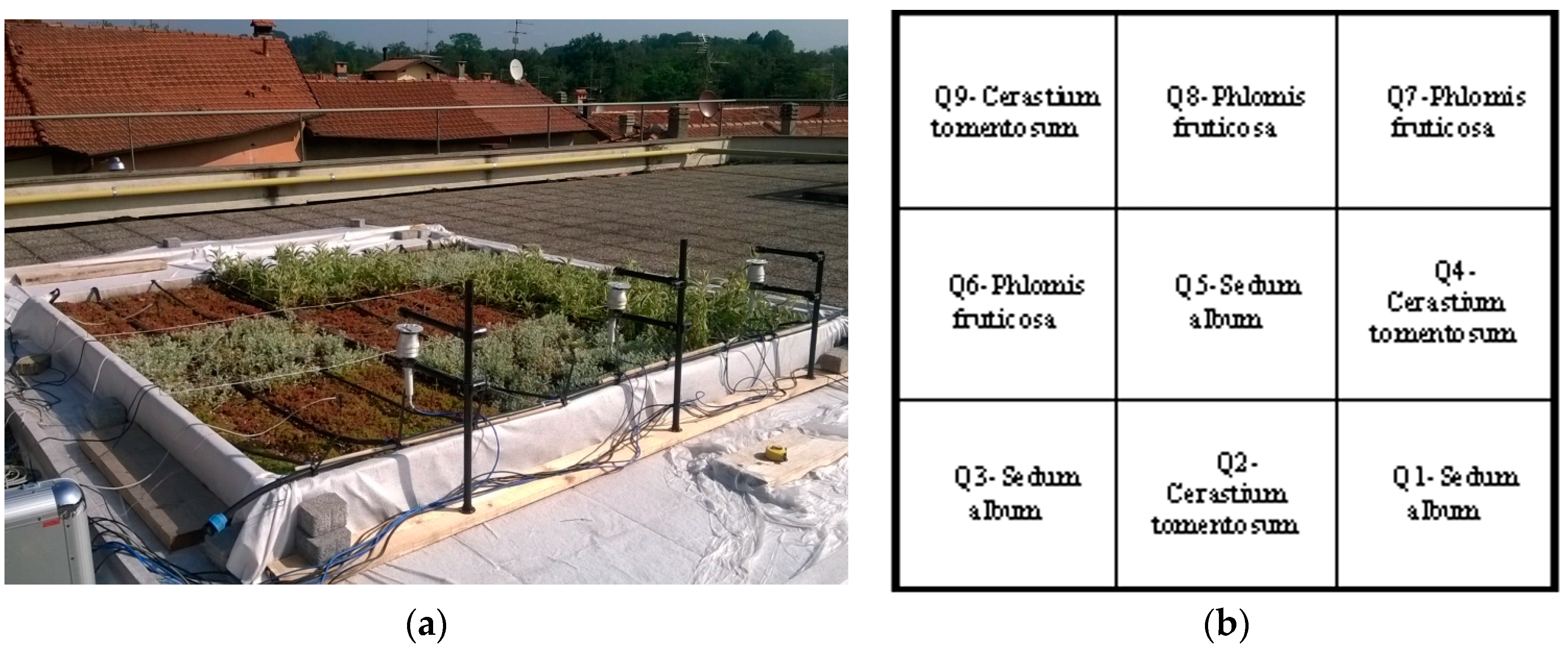
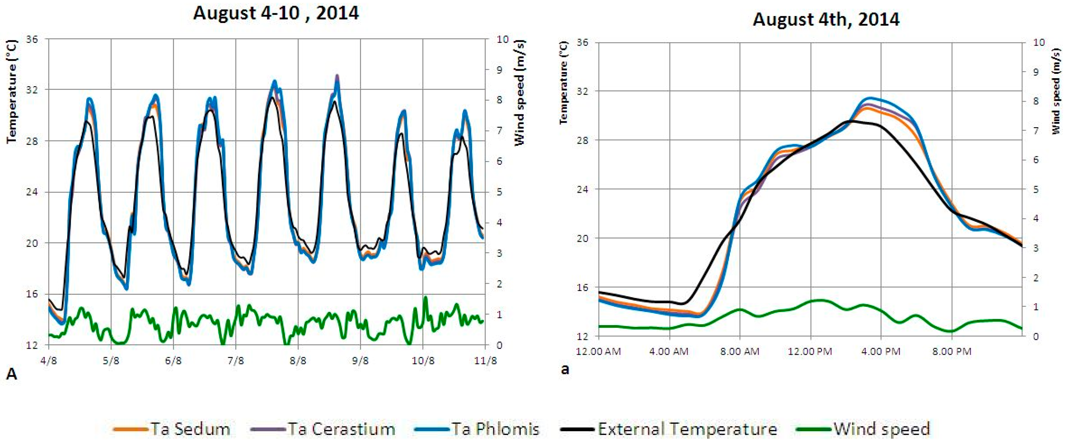
Figure 8 shows trends relating to the monitoring of air temperatures (T_a) at a height of 30 cm from the cultivation surface in three plots (Q1, Q4, and Q7, see Figure 2a,b), with respect to a sample week (Figure 8A) and a reference day (Figure 8a). Trends shown in Figure 8 are also confirmed for the whole monitoring period.

The evapotranspiration depends on solar radiation, water content in the growing medium, vegetation’s density and height [35], and wind velocity and air humidity [36]. Silva et al. [35], demonstrate, through numerical analyses, that for each typology of green roof (extensive, intensive, and semi-intensive), evapotranspiration is more relevant in summer months (May–September), during which solar radiation is higher. When comparing extensive with intensive green roof solutions, evapotranspiration is higher for intensive green roofs that have a thicker substrate and higher plants [35].

Figure 8A shows the outdoor air temperatures (T_a) at a height of 30 cm from the cultivation surface, whilst following the outdoor temperature (T_e) trend, its peaks amplify: T_a is, in fact, lower than T_e at night and higher in the daytime, with a phase shift of about two hours. Cerastium is the species that shows the most sensitive difference between Ta and T_s both at night (−3.2 °C) and during daytime (+3.3 °C), followed by Phlomis with a thermal gradient of −3.2 °C at night and 3.1 °C during daytime, and by Sedum with −2.8 °C at night and +2.7 °C during daytime. The behavior at night is as expected in relation to UHI phenomenon characterized by higher temperatures at night due to the release of the heat accumulated during daytime [37]. During daytime, instead, the positive effects depend on the evapotranspiration phenomenon are not sensitive due to both small-size crops and a low water content of the growing medium.

The wind speed parameter is considered not sensitive, because of the low values reached (<2 m/s).

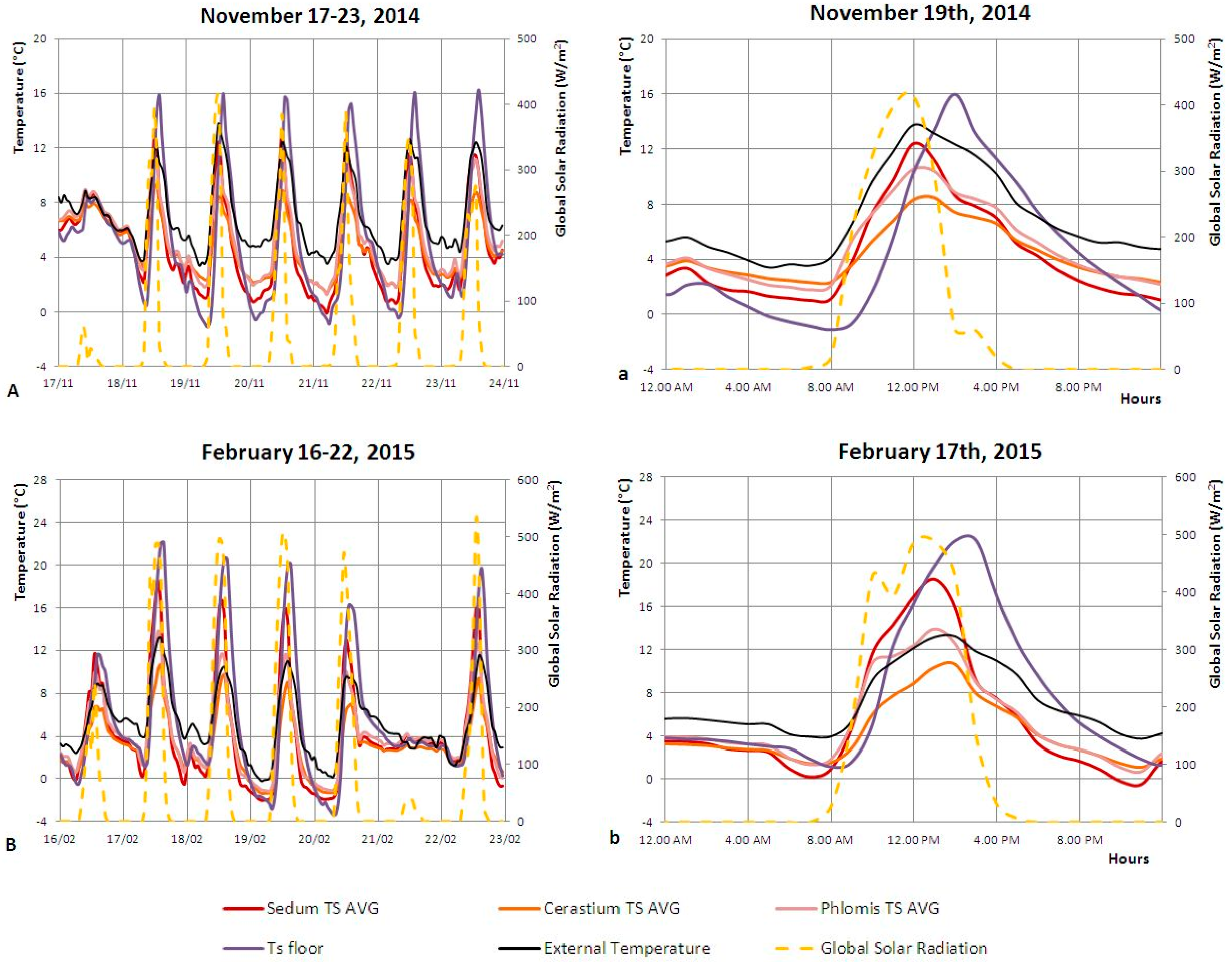
3.1.2. Autumn 2014 and Winter 2014–2015

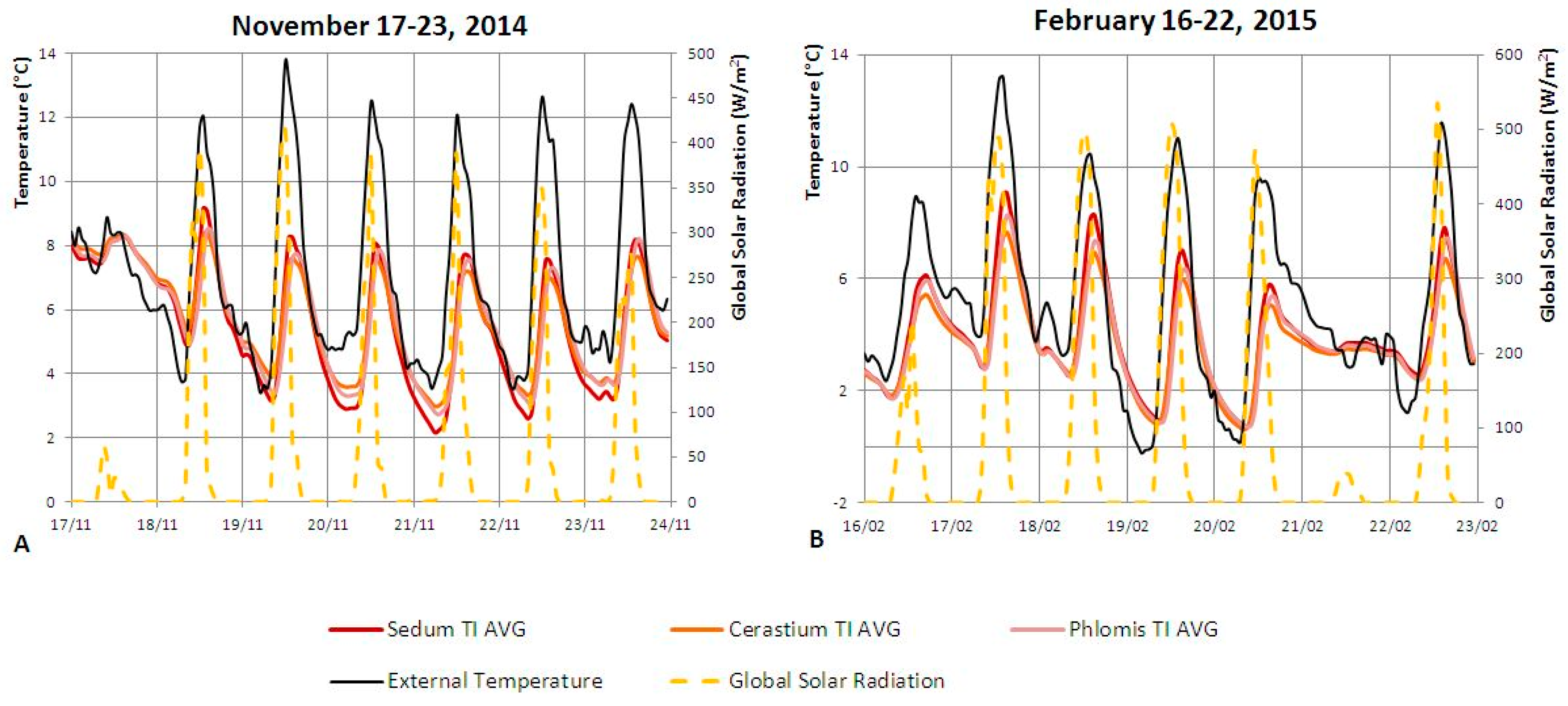
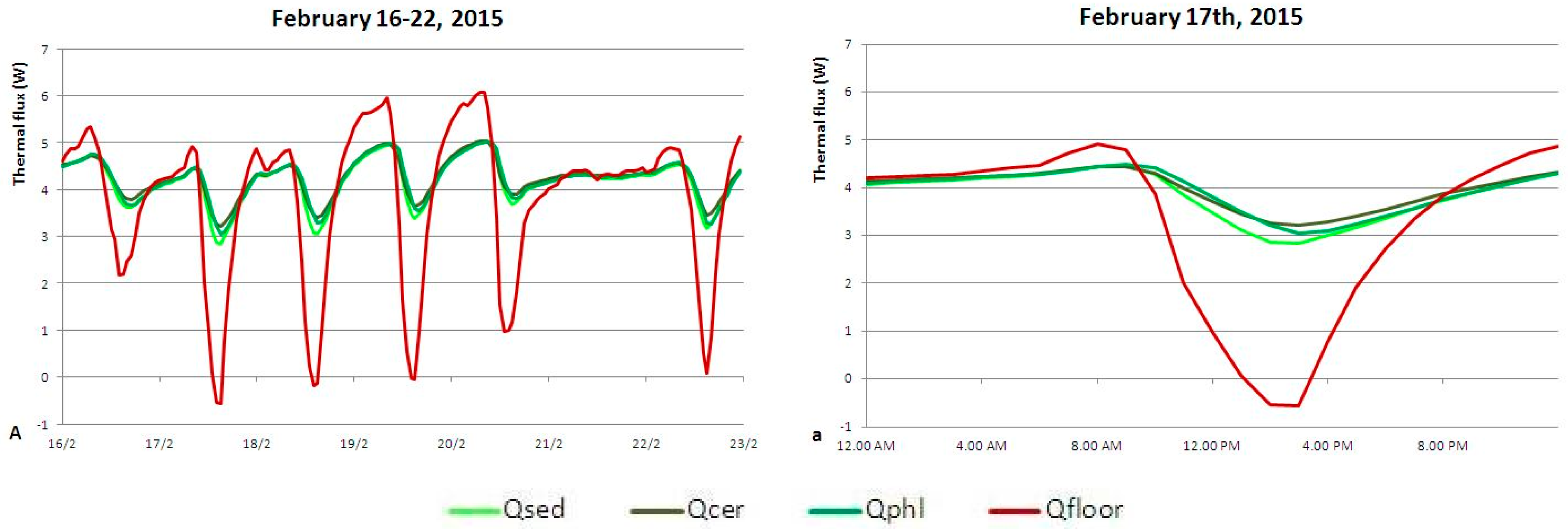
Figure 9 shows graphs related to the surface temperatures of the three plant species as a function of both the external temperature (T_e) and the global solar radiation (I) with respect to two reference weeks, from 17–24 November 2014 (Figure 9A,a), representative of autumn 2014, and from 16–22 February 2015 (Figure 9B,b), representative of winter 2014–2015.

The sample days shown in graphs Figure 9a,b were chosen as a function of similar outdoor conditions in terms of outdoor temperature (14 °C of peak) and solar radiation level (500 W/m²).

Even in the presence of small levels of global solar radiation, the surface temperature of the plant species (T_s) is a function of it, strongly depending on the shading attitude of the different plant species. In November (A,a), the growth of the initial planting allows to analyze temperatures trends during spring 2015 (Figure 5B,b), even if to lesser degree of accuracy: on 19 November Sedum and Phlomis show surface temperatures that are, respectively, 4.1 °C and 2.2 °C higher than Cerastium (at solar radiation peak). It is very interesting to observe how Sedum, maybe due to its creeping development, shows the same behavior of the paved surface, with surface temperatures that are lower at night and higher during daytime (Figure 9a). In February 2015, differences between the temperatures of the three species are more marked: surface temperature differences between Sedum and Phlomis, with respect to Cerastium, are 8.2 °C and 3.5 °C higher, respectively (Figure 9b).

The correlation index was calculated for wintertime too (

Table 5. The Pearson’s r between (T_s) and (I), and between (T_s) and (T_e), calculated considering three global solar radiation intervals.

Pearson’s r	Global Solar Radiation
between Ts and I	0–200 W/m2	400–500 W/m2	600–700 W/m2
Sedum	0.23	−0.39	1
Cerastium	0.12	−0.41	1
Phlomis	0.19	−0.33	1
between Ts and Te
Sedum	0.98	0.80	1
Cerastium	0.97	0.88	1
Phlomis	0.98	0.85	1

), considering three different global solar radiation intervals (0–200, 400–500, and 600–700 (during the sampling period (months of November 2014 and February 2015), the highest value reached by the global solar radiation was 647 W/m²) W/m², respectively) at solar peak. A sampling period of 58 days was considered (months of November 2014 and February 2015).

First of all, the analysis of the correlation indexes between the surface temperatures of the plant species (T_s) and the external temperature (T_e) shows a strong direct correlation (Pearson’s r > 0.7) for all the global solar radiation intervals. Secondly, the correlation between (T_s) and (I) is: direct and not sensitive (Pearson’s r < 0.3) between 100 W/m² and 200 W/m²; negative and moderate around 500W/m², and positive and strong (0.8 < Pearson’s r < 1) for I > 500W/m².

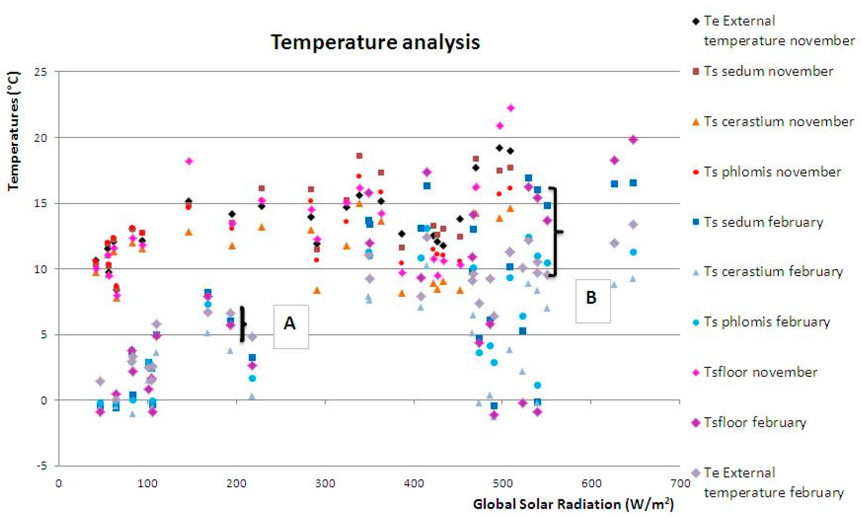
Instead, Figure 10 shows the relationship, in terms of thermal gradient, between the surface temperatures of the plant species (T_s), the external temperature (T_e) and the global solar radiation (I), during daily solar peak (about 12:30 p.m.). The considered sampling period is 58 days (months of November 2014 and February 2015).

The surface temperatures of the plant species (T_s) differ from the external temperature (T_e) with a thermal gradient on average lower than 5 °C (‘A’ data in Figure 10) for low values of solar radiation (I < 500 W/m²). Therefore, the surface temperatures of the plant species (T_s) differ from the external temperature (T_e) with thermal gradients of about 10 °C (‘B’ data in Figure 10) for high values of solar radiation (I > 500 W/m²). The trend is the same during summer and spring seasons, even with lower values in autumn and winter.

Therefore, the same conclusions reached on the basis of summer/spring data can be confirmed for autumn/winter data: the external temperature (T_e) affects the seasonal peak value of the surface temperature of the plant species (T_s), while the global solar radiation determines the thermal gradient between T_s and T_e.

Although the solar radiation peak reaches an energy value of about 500 W/m², significantly lower than it the spring/summer season, the thermal gradient between the planted plots T_s and the surface temperature of the paved cover (T_sfloor) of the terrace on which the experimental set-up is positioned, is marked.

Table 6. Surface thermal gradients between the surface temperature of the plant species (T_s) and the paved surface temperature (T_sfloor), 19 November 2014 and 17 February 2015.

Ts	Sedum	Cerastium	Phlomis	Year
Ts−Tsfloor	−4	−7.5	−6	2014
Ts−Tsfloor	−4	−12	−8.5	2015

briefly summarizes thermal gradients between plots (T_s) and paved surface (T_sfloor).

With regard to the inside temperature (T_i) trends, Figure 11 shows the related graphs.

Inside temperature trends reflect the outdoor ones: Sedum T_i is higher than the two other planted species, followed by Phlomis. Differences are, however, slight (about 0.5 °C) and inside temperatures tend to overlap, due to a very low thermal gradient.

Table 7. Thermal gradients between the paved surface T_sfloor, plots T_s and T_i.

dT 2014	Sedum	Cerastium	Phlomis	dT 2015	Sedum	Cerastium	Phlomis
Ts−Tsfloor	−4	−7.5	−6	Ts−Tsfloor	−4	−12	−8.5
Ti−Tsfloor	−7.5	−8.5	−8	Ti−Tsfloor	−13.5	−15	−14
Ti−Ts	−3.5	−1	−2	Ti−Ts	−9.5	−3	−5.5

summarizes the comparison between inside temperatures of the plot (T_i) and paved surface temperatures (T_sfloor), under solar radiation.

3.2. Considerations Concerning the Relationship between Plant Species and Surface Temperatures

The monitored data had primarily underlined a very interesting aspect regarding the relationship between the variation of surface temperatures of the planted areas and the related thermal gradients with respect to the coverage in concrete tiles and mineral grit of the terrace, and the global solar radiation.

Table 8. Surface temperatures thermal gradients (T_s) as a function of the solar radiation level (I).

Global Solar Radiation		Clear Sky		Light Fog		Cluody		Yellow Disc		White Disc		Perceptible Sun		Thick Fog
		(1000–600 W/m2)		(600–500 W/m2)		(500–400 W/m2)		(400–300 W/m2)		(300–200 W/m2)		(200–100 W/m2)		(100–50 W/m2)
		Min	Max	Min	Max	Min	Max	Min	Max	Min	Max	Min	Max	Min	Max
Summer 2014	Tsfloor−Ts,sed	5	14	6	11	3	5	−1	2			0	2
	Tsfloor−Ts,cer	7	16	7	12	5	6	1	3			1	3
	Tsfloor−Ts,phl	10	20	9	12	5	7	2	4			0	2
Autumn 2014	Tsfloor−Ts,sed	5	10	9	10	3	5	5	3	1	0	1	0.5	0	−1.5
	Tsfloor−Ts,cer	8	13	10	12	7	7	7	4	2	1	2	2.5	1	−0.5
	Tsfloor−Ts,phl	8	14	11	12	5	6	6	3	1	1	1	11.5	0	−1.5
Winter 2014–2015	Tsfloor−Ts,sed	6	6	3	3	6	4	−8	3	0		1	1	−0.5	3
	Tsfloor−Ts,cer	13	16	9	10	11	10	6	8	5		3	5	0.5	4
	Tsfloor−Ts,phl	12	10	6	8	9	8	4	5	2		2	2	−0.5	3
Spring 2015	Tsfloor−Ts,sed	6	0	1	5	0	1	1		0	0	0
	Tsfloor−Ts,cer	14	18	6	9	6	6	5		3	1	1
	Tsfloor−Ts,phl	11	17	5	8	2	5	3		2	0	0

shows thermal gradients between the surface temperatures of the planted area and paved surface, at solar radiation peaks.

In order to achieve the values contained in Table 8, solar radiation peak values were considered along the 292 days of the experimental campaign, from 23 July 2014 to 10 May 2015, at which surface temperatures of the three plant species (in term of plot average for each of them) and of the pavement were measured, than thermal gradients that were calculated at the minimum and maximum surface temperature values.

Tabulated results underline how an appropriate selection of the vegetative solutions could contribute to significantly reducing the external surface temperatures (about 10 °C–20 °C for solar radiation values I > 500 W/m² and less than 6 °C for I < 500 W/m², irrespective of the season) compared to a flat walkway rooftop. In the winter season, depending on reduced values of both solar radiation and external temperatures (T_e), the surface temperatures of the planted plots (T_s) show, practically, a zero thermal gradient compared to the terrace, except with particular improved conditions, due to the transpiration of plants which increases temperatures by about half a degree.

3.3. Considerations Concerning Ts and Ti with Respect to Building Materials Durability

Surface layers of a green roof allow the sensible reduction in the thermal stresses to which the building roofing materials are subjected [21,23].

Analyzing maximum and minimum temperatures reached on the surface, and inside by the growing medium, with respect to the paved surface of the terrace, on a summer day characterized by extreme outdoor conditions (4 August 2014,

Table 9. Thermal gradients—4 August 2014.

Plant Species	Ts (°C)			Ti (°C)			Ts pav (°C)
	Min	Max	Δ	Min	Max	Δ	Min	Max	Δ
Sedum	14.7	35.3	20.6	16.7	27.2	10.5	13.3	45.2	31.9
Cerastium	14.2	33.3	19.1	16.1	27.9	11.8
Phlomis	15.2	28.3	13.1	16.2	24.8	8.6

), the traditional roofing system shows a thermal gradient of about 32 °C, while surface temperatures are 20 °C higher than the most unfavorable case (Sedum), and inside temperatures about 12 °C higher than Cerastium.

During a winter day, characterized by extreme outdoor conditions (2 February 2015,

Table 10. Thermal gradients—2 February 2015.

Plant Species	Ts (°C)			Ti (°C)			Ts pav (°C)
	Min	Max	Δ	Min	Max	Δ	Min	Max	Δ
Sedum	−3.2	6.6	9.8	−0.4	0.0	0.4	−5.9	15.3	21.2
Cerastium	−2.1	1.8	3.9	−0.6	0.6	1.2
Phlomis	−2.8	4.2	7	−0.4	−0.3	0.1

), the traditional roofing system reaches a minimum temperature of −2.9 °C and a maximum temperature of 21.2 °C.

If the surface temperatures of the growing medium are subject to a maximum thermal gradient of approximately 10 °C in the case of Sedum, the inside temperatures of all three species are almost constant.

The smaller the thermal fluctuations, the greater the building materials durability, in favor of a reduction of ordinary and extraordinary maintenance costs.

3.4. Considerations Concerning Ti with Respect to Energy Saving

Low values, which are barely affected by large fluctuations of surface temperatures thermal gradient values, involve a reduction of heat losses during winter and overheating in summer of the indoor areas, which leads to a reduction of energy consumption.

3.4.1. Summer Season

During the summer season, the shading and protection action of a retrofit green roof (anti-root layer, growing medium, and vegetative layer) corresponds to a reduction of the surface temperatures of the upper side of the underneath of the growing medium (T_un), with respect to the surface temperatures (T_sfloor) of the paved surface of the terrace, exposed to direct solar radiation.

The contribution provided by the combination of growing medium plus the vegetative layer could be quantified by calculating the incoming heat flow during exposure to direct solar radiation and comparing it with the thermal flow of the roofing system with only the current walkable flooring system, according to the following equation [19]:

$${\mathrm{q}}_{\mathrm{ij}}={\left[\frac{\left(\mathrm{Ts}-\mathrm{Tin}\right)}{\mathrm{R}}\right]}_{\mathrm{ij}}$$

(1)

where T_s is, alternatively, the surface temperature of the paved terrace (T_sfloor) when the heat flow is calculated considering the roof system without the contribution of a green roof, or the underneath temperature (T_un) when the calculation involves the planted plots under study; T_in represents the indoor air temperature of the spaces under the roof, characterized by a cooling set-point of 26 °C; R is the roof thermal transmittance, equal to 0.26 W/m²K, according to the national legislation in force for roofing systems, for Italian climatic zone E [13].

The roof thermal resistance is assumed the same for both configurations—with and without the green roof (growing medium + plant species)—considering that the green roof contribution is quantified by the difference between the underneath temperature (T_un) and the surface temperature of the paved terrace (T_sfloor). Therefore, both of the variables, namely the shielding contribution of plant species (depending on the season and the leaf development) and the growing medium thermal insulation (as a function not only of the thermal conductivity of the substrate, but also to its moisture level), are quantified due to their effective contribution.

The calculated results are represented graphically in Figure 12.

The most interesting aspect that emerges from Figure 12a, is that during direct solar radiation hours (from 8:00 a.m. to 8:00 p.m.) the heat flow into the roof system without the protection of growing medium plus vegetative layer is markedly higher, causing the underlying indoor environments to overheat, and a simultaneous increase in cooling energy consumption; on the contrary, at night the trends are almost the same, even if they show a slightly worse performance compared to that of the original terrace roofing system. The graph shows how the indoor radiative heat phenomena worsen markedly, due to the roofing system high insulation level.

3.4.2. Winter Season

It is particularly interesting to underline that during the winter season it was verified that the daytime protective behavior from solar heat gains did not involve a sensitive improvement of daily overheating gains.

Figure 13 graphically summarizes the calculation results.

Figure 13a shows how at night energy behavior is almost the same, thanks to the high level of roofing system insulation. The alleged loss of solar heat gains occurs during daylight hours, but this behavior is only temporary (about 4 h) and it is less sensitive considering a radiation exposure of about 550 W/m².

Instead, on semi-sunny or overcast days (22 February 2015, Figure 13A), heat flows are the same and involve the same heating energy consumption.

4. Conclusions

The main goal of the present study is the analysis of the energy and environmental impact caused by the choice of different plant species as vegetation solutions for green roofs, through the study of parameters, such as surface and inside growing medium temperatures.

The majority of studies in the literature refer to numerical simulations concerning the overall performances of a green roof compared to a traditional one. Following this approach, the contribution of each stratigraphic layer is not taken into account separately, and the calculations must be repeated for each different green roof configuration.

The present study involves on-site monitoring, like a few studies found in the literature. Some studies [18,19,22,23,26,35] refer to experimental monitoring tests similar to those of the present study, however their goals are very different. For example, Teemusk and Mander [23] relate monitoring campaigns aimed to investigate the overall behavior of a green roof; Niachou et al. [18], Santamouris et al. [26], and Silva et al. [35] use the monitored data to validate energy simulation and mathematical models, or to provide a baseline comparison for future analysis [22]. In Celik et al. [19], different kinds of growing media and plant species, which are considered to form a combined domain for the purpose of thermal analysis, were combined in multiple different configurations. However, this approach undermines the study of the single plant species because their performances are combined with different types of growing media.

The presented study has identified, quantified and compared, by way of the results of the monitoring test campaign, the specific contribution of three different plant species for green roofs, assuming the other variables to be unchanged. The three plant species were selected as species suited to the climate of Northern Italy, belonging to xerophytic environments.

First of all, the methodological approach of the present study allows to study the specific functionality of each single species. This confirms the results of the study of Lundholm et al. [17] who found that when different species are planted in the same plot, the functionality of the best individual species is reduced because they are sharing the plot with species that perform worse.

On the other hand, the present approach demonstrates the specific potential of the plant species in decreasing surface temperatures and inside temperatures of the growing medium and, consequently, reducing their impact in managing roof inside/outside heat flows and urban heat island phenomenon (UHI).

The main conclusions, drawn from the analysis of the monitoring data collected during the whole experimental campaign, are schematically summarized below:

• relationship between T_s and UHI: the surface temperatures of the plant species (T_s)—closely connected with the choice of the specific vegetative species—mainly affect outward heat flows (mitigation of local and global UHI phenomena);
• the plant species surface temperature (T_s) is a direct function of both the global solar radiation (I)—and, consequently, of the shading potential of each plant species—and of the external temperature (T_e), as shown in Table 2 and Table 5. Actually, in considering the Pearson’s correlation coefficient, during the summer 2014/spring 2015 configuration period there is a direct correlation (Pearson’s r > 0) between the surface temperatures of the plant species (T_s) and the external temperature (T_e); moreover, the more the global solar radiation increases, the more the correlation between the surface temperatures of the plant species (T_s) and the external temperature (T_e) decreases. Secondly, the correlation between (T_s) and (I) is direct, increasing, and sensitive (0.8 < Pearson’s r < 1) between 100 W/m² and 800 W/m²; conversely, considering very high values of global solar radiation (I > 800 W/m²), the correlation decreases. Concerning the autumn 2014/winter 2015 configuration period, the analysis of the correlation indexes between the surface temperatures of the plant species (T_s) and the external temperature (T_e) show a strong direct correlation (Pearson’s r > 0.7) for all the global solar radiation intervals. Whereas, the correlation between (T_s) and (I) is: direct and not sensitive (Pearson’s r < 3) between 100 W/m² and 200 W/m²; negative and moderate around 500W/m², and positive and strong for I > 500W/m²;
• the external temperature (T_e) affects the seasonal peak value of the surface temperature of the plant species (T_s); conversely, the global solar radiation (I) determines the thermal gradient between T_s and T_e;
• the inside temperature of the growing medium (T_i) depends on the shading potential of the chosen vegetative species;
• according to some studies (e.g., [21,22,23]), Ti strongly affects the durability of the underlying building materials (such as waterproofing membranes);
• according to some studies (e.g., [4,21]), cooling loads are considerably reduced in summer; and
• in winter, both thermal and energy performances deteriorate as a function of the seasonal solar radiation level (Figure 13), although this issue is of relatively small importance at our latitudes.

Surface temperature T_s trends, as a function of plant species, appreciably influence the reduction of urban overheating (mitigation of the UHI phenomenon), while the reduction of summer heat gains is practically the same, because inside temperatures under the growing medium tend to coincide, independently, from the planted vegetative species.

According to Sailor [38], the reduction of thermal loads depends more on the growing medium thickness than on the planted vegetative solutions. In winter, considering surface temperatures, a green roof could reduce daily solar heat gains as a function of the seasonal solar radiation level while, at night, it behaves just like a properly insulated roof.

5. Future Works

In light of the obtained results, the authors intend to carry on with this research in order to quantify the actual energy provided by every single green roof layer [19] through both laboratory and on-site monitoring experimental campaigns. A specific experimentation focused on the monitoring of three different roofing systems is currently under way. The roofing systems are characterized as follows: the first is a ‘complete’ green roof; the second is the same green roof with or without the vegetative layer (only growing medium); and the third has no vegetative layer and no growing medium (only the drainage layer protected by a white non-woven fabric). The monitoring of energy consumptions for summer cooling and winter heating, together with the analysis of both surface temperatures trends of each roofing layer and related heat flows, will allow further extension of the observations made so far. Furthermore, the tests for measuring the growing medium thermal resistance calculated on site will be compared with some laboratory tests carried out in steady-state conditions, to define a series of values to be used during the design phase as a function of the type of growing medium and degree of internal moisture.

References

1. Ascione, F.; Bianco, N.; de’ Rossi, F.; Turni, G.; Vanoli, G.P. Green roofs in European climates. Are effective solutions for the energy savings in air-conditioning? Appl. Energy 2013, 104, 845–859. [Google Scholar] [CrossRef]
2. Garrison, N.; Horowitz, C. Looking Up: How Green Roofs and Cool Roofs Can Reduce Energy Use, Address Climate Change and Protect Water Resources in Southern California; NRDC Report; Natural Resources Defense Council: California, CA, USA, 2012.
3. Wong, N.H.; Cheong, D.K.W.; Yan, H.; Soh, J.; Ong, C.L.; Sia, A. The effects of rooftop garden on energy consumption of a commercial building in Singapore. Energy Build. 2003, 35, 353–364. [Google Scholar] [CrossRef]
4. Castleton, H.F.; Stovin, V.; Beck, S.B.M.; Davison, J.B. Green roofs; building energy savings and the potential for retrofit. Energy Build. 2010, 42, 1582–1591. [Google Scholar] [CrossRef]
5. Jaffal, I.; Ouldboukhitine, S.-E.; Belarbi, R. A comprehensive study of the impact of green roofs on building energy performance. Renew. Energy 2012, 43, 157–164. [Google Scholar] [CrossRef]
6. Yang, H.S.; Kang, J.; Choi, M.D. Acoustic effects of green roof systems on a low-profile structure at street level. Build. Environ. 2012, 50, 44–55. [Google Scholar] [CrossRef]
7. Van Renterghem, T.; Botteldooren, D. Numerical evaluation of sound propagating over green roofs. J. Sound Vib. 2008, 317, 781–799. [Google Scholar] [CrossRef]
8. Bradley Rowe, D. Green roofs as a means of pollution abatement. Environ. Pollut. 2011, 159, 2100–2110. [Google Scholar] [CrossRef] [PubMed]
9. Akbari, H.; Pomerantz, M.; Taha, H. Cool surfaces and shade trees to reduce energy use and improve air quality in urban areas. Solar Energy 2001, 70, 295–310. [Google Scholar] [CrossRef]
10. Curriero, F.C.; Heiner, K.S.; Samet, J.M.; Zeger, S.L.; Strug, L.; Patz, J.A. Temperature and morality in 11 cities of the eastern United States. Am. J. Epidemiol. 2002, 155, 80–87. [Google Scholar]
11. Susca, T. Multiscale approach to life cycle assessment. Evaluation of the effect of an increase in New York City’s rooftop albedo on human health. J. Ind. Ecol. 2012, 16, 951–962. [Google Scholar] [CrossRef]
12. Alexandri, E.; Jones, P. Temperature decreases in an urban canyon due to green walls and green roofs in diverse climates. Build. Environ. 2008, 43, 480–493. [Google Scholar] [CrossRef]
13. DM 26 June 2015, Schemes and reference procedures for drawing up the draft technical report for the purpose of the requirements and the application of the minimum energy performance of buildings, Annex 2, Gazzetta Ufficiale della Repubblica Italiana. 2015. Available online: http://www.gazzettaufficiale.it/eli/id/2015/07/15/15A05199/sg (accessed on 26 August 2016).
14. Versini, P.A.; Jouve, P.; Ramier, D.; Berthier, E.; de Gouvello, B. Use of green roofs to solve storm water issues at the basin scale—Study in the Hauts-de-Seine county. Urban Water J. 2015, 13, 1–10. [Google Scholar] [CrossRef]
15. Hashem, A.; Rose, L.S. Urban surfaces and heat island mitigation potentials. J. Hum. Environ. Syst. 2008, 11, 85–101. [Google Scholar]
16. Saadatian, O.; Sopian, K.; Salleh, E.; Lim, C.H.; Riffat, S.; Saadatian, E.; Toudeshki, A.; Sulaiman, M.Y. A review of energy aspects of green roofs. Renew. Sustain. Energy Rev. 2013, 23, 155–168. [Google Scholar] [CrossRef]
17. Lundholm, J.; MacIvor, J.S.; MacDougall, Z.; Ranalli, M. Plant species and functional group combinations affect green roof ecosystem functions. PLoS ONE 2010, 5, 1–11. [Google Scholar] [CrossRef] [PubMed]
18. Niachou, A.; Papakonstantinou, K.; Santamouris, M.; Tsangrassoulis, A.; Mihalakakou, G. Analysis of the green roof thermal properties and investigation of its energy performances. Energy Build. 2001, 33, 719–729. [Google Scholar] [CrossRef]
19. Celik, S.; Retzlaff, W.A.; Morgan, S. Evaluation of energy savings for buildings with green roofs having different vegetation. In Proceedings of the International High Performance Buildings Conference, Purdue, IN, USA, 12–15 July 2010; p. 24.
20. Arabi, R.; Shahidan, M.F.A.; Kamal, M.S.M.; Ja’afar, M.F.Z.B.; Rakhshandehroo, M. Mitigating urban heat island through green roofs. Curr. World Environ. 2015, 10, 918–927. [Google Scholar] [CrossRef]
21. Liu, K.; Baskaran, B. Thermal performance of green roofs through field evaluation. In Proceedings of the First North American Green Roof Infrastructure Conference, Awards and Trade Show, Chicago, IL, USA, 29–30 May 2003.
22. Liu, K.; Minor, J. Performance evaluation of an extensive green roof. In Proceedings of the Greening Rooftops for Sustainable Communities Conference, Washington, DC, USA, 5–6 May 2005.
23. Teemusk, A.; Mander, U. Green roof potential to reduce temperature fluctuations of a roof membrane: A case study from Estonia. Build. Environ. 2009, 44, 643–650. [Google Scholar] [CrossRef]
24. Klysik, K.; Fortuniak, K. Temporal and spatial characteristics of the urban heat island of Lodz Poland. Atmos. Environ. 1999, 33, 3885–3895. [Google Scholar]
25. Rosenzweig, C.; Solecki, W.D. Mitigating New York City’s heat island with urban forestry, living roofs, and light surfaces. In New York City Regional Heat Island Initiative Final Report; NYSERDA: New York City, NY, USA, 2010. [Google Scholar]
26. Santamouris, M.; Pavlou, C.; Doukas, P.; Mihalakako, G.; Synnefa, A.; Hatzibiros, A.; Patargias, P. Investigating and analyzing the energy and environmental performance of an experimental green roof system installed in a nursery school building in Athens, Greece. Energy 2007, 32, 1781–1788. [Google Scholar] [CrossRef]
27. D.P.R. 26 August 1993, n. 412. Regulation on standards for the design, installation, operation and maintenance of heating systems in buildings in order to limit energy consumption, implementing art. 4, paragraph 4, Law 10, 9 January 1991. Available online: http://www.gazzettaufficiale.it/eli/id/1993/10/14/093G0451/sg (accessed on 26 August 2016).
28. D.Lgs. 19 August 2005, n. 192. “Attuation of the European Directive 2002/91/EU concerning the energy efficiency in buildings”, and D.Lgs. 29 December 2006, n. 311. Available online: http://www.gazzettaufficiale.it/atto/serie_generale/caricaDettaglioAtto/originario?atto.dataPubblicazioneGazzetta=2007-02-01&atto.codiceRedazionale=007G0007 (accessed on 26 August 2016).
29. Olivieri, M.; Zaffagnini, T. Superfici Vegetali Applicate All’involucro Edilizio per il Controllo Microclimatico Dell’ambiente Costruito. Ph.D. Thesis, Università di Ferrara, Ferrara, Italy, 2009. [Google Scholar]
30. Provenzano, M.E.; Cardarelli, M.; Saccardo, F.; Colla, G.; Battistelli, A.; Proietti, S. Evaluation of perennial herbaceous species for their potential use in a green roof under mediterranean climate conditions. Acta Hortic. 2010, 881, 661–667. [Google Scholar] [CrossRef]
31. Khalaf, M.K.; Stace, C.A. The distinction between Cerastium tomentosum L. and C. biebersteinii DC. (Caryophyllaceae), and their occurrence in the wild. Br. Watsonia 2001, 23, 481–491. [Google Scholar]
32. Iovi, K.; Kolovou, C.; Kyparissis, A. An ecophysiological approach of hydraulic performance for nine Mediterranean species. Tree Physiol. 2009, 29, 889–900. [Google Scholar] [CrossRef] [PubMed]
33. Nesa Datalogger. Available online: http://www.nesasrl.eu/it/datalogger_tmf500.aspx.
34. Enea Archivio Climatico. Available online: http://clisun.casaccia.enea.it/Pagine/Index.htm.
35. Silva, C.M.; Gomes, M.G.; Silva, M. Green roofs energy performance in Mediterranean climate. Energy Build. 2016, 116, 318–325. [Google Scholar] [CrossRef]
36. Allen, R.G.; Pereira, L.S.; Raes, D.; Smith, M. Crop Evapotranspiration—Guidelines for Computing Crop Water Requirements; FAO Irrigation and Drainage Paper 56; FAO: Roma, Italy, 1998. [Google Scholar]
37. Oke, T.R. Canyon geometry and the urban heat island: Comparison of scale model and field observations. J. Climatol. 1981, 1, 237–254. [Google Scholar] [CrossRef]
38. Sailor, D.J. A green roof model for building energy simulation programs. Energy Build. 2008, 40, 1466–1478. [Google Scholar] [CrossRef]
Figure 1. Imagine of the roof terrace of Fondazione Minoprio.
Buildings 06 00033 g001
Figure 2. Imagine of: (a) the measurement area; and (b) scheme of the plant species planting.
Buildings 06 00033 g002
Figure 3. Plots monitoring scheme. Left side: plot area example; center: cross-section of the monitoring scheme—plot area; right side: cross-section of the monitoring scheme—terrace.
Buildings 06 00033 g003
Figure 4. Surface temperature sensor installed on the flat roof (Tsfloor) and solarimeter.
Buildings 06 00033 g004
Figure 5. Ts analysis as a function of the global solar radiation and the external temperature (Te): (A,a) summer 2014; (B,b) spring 2015. Upper case letters refer to the reference week, while lower case letters refer to the reference day.
Buildings 06 00033 g005
Figure 6. Analysis of the surface temperatures of the plant species (Ts) as a function of the global solar radiation and the external temperature.
Buildings 06 00033 g006
Figure 7. Trend of the inside temperatures of the growing medium (Ti) as a function of the global solar radiation and the external temperature: (A) summer 2014; and (B) spring 2015.
Buildings 06 00033 g007
Figure 8. Air temperatures trend (Ta), at a height of 30 cm from the planting surface: (A) sample week, from 4–10 August 2014; (a) sample day, 4 August 2014.
Buildings 06 00033 g008
Figure 9. Ts analysis as a function of the global solar radiation and the external temperature: (A,a) autumn 2014; (B,b) winter 2014–2015. Upper case letters refer to the reference week, while lower case letters refer to the reference day.
Buildings 06 00033 g009
Figure 10. Ts analysis as a function of the global solar radiation.
Buildings 06 00033 g010
Figure 11. Inside temperature of the growing medium (Ti) trend as a function of the global solar radiation (W/m2) and the external temperature (Te): (A) autumn 2014; (B) winter 2014–2015.
Buildings 06 00033 g011
Figure 12. Analysis of summer heat flows: (A) sample week; (a) sample day.
Buildings 06 00033 g012
Figure 13. Analysis of winter heat flows: (A) sample week; (a) sample day.
Buildings 06 00033 g013